Multi-frequency polarimetry of the Galactic radio background around 350 MHz: II. A region in Horologium around
l = 137°, b = 7°

We study a conspicuous ring-like structure with a radius of about 1.4° which was observed with the Westerbork Synthesis Radio Telescope (WSRT) at 5 frequencies around 350 MHz. This ring is very prominent in Stokes $Q$ and $U$, and less so in polarized intensity $P$. No corresponding structure is visible in total intensity Stokes $I$, which indicates that the ring is created by Faraday rotation and depolarization processes. The polarization angle changes from the center of the ring outwards to a radius $\,\hbox{\hbox to0.0pt{\hbox{\lower 4.0pt\hbox{$\sim$}}\hss} \lower-1.0pt\hbox{$>$}}\,1.7\degr$. Thus, the structure in polarization angle is not ring-like but resembles a disk, and it is larger than the ring in $P$. The rotation measure $RM$ decreases almost continuously over the disk, from $RM$ $\approx 0$ rad m^-2 at the edge, to $-8$ rad m^-2 in the center, while outside the ring the $RM$ is slightly positive. This radial variation of $RM$ yields stringent constraints on the nature of the ring-like structure, because it rules out any spherically symmetrical magnetic field configuration, such as might be expected from supernova remnants or wind-blown bubbles. We discuss several possible connections between the ring and known objects in the ISM, and conclude that the ring is a predominantly magnetic funnel-like structure. This description can explain both the field reversal from outside to inside the ring, and the increase in magnetic field, probably combined with an electron density increase, towards the center of the ring. The ring-structure in $P$ is most likely caused by a lack of depolarization due to a very uniform $RM$ distribution at that radius. Beyond the ring, the $RM$ gradient increases, depolarizing the polarized emission, so that the polarized intensity decreases. In the southwestern corner of the field a pattern of narrow filaments of low polarization, aligned with Galactic longitude, is observed, indicative of beam depolarization due to abrupt changes in $RM$. This explanation is supported by the observed $RM$.

1 Introduction

Observation of the diffuse polarized background of our Galaxy at radio frequencies provides a unique way to observe features in the ISM that are otherwise invisible. In this paper we report and analyze the detection in radio polarization of a remarkable circular structure with a radius of $\sim 1.4\degr$. The observed radiation is synchrotron radiation, originating from relativistic cosmic ray electrons in interaction with the Galactic magnetic field. The linearly polarized component of the synchrotron radiation is modulated by several mechanisms, among which Faraday rotation, viz. the birefringence of left- and right-handed circularly polarized radiation in a medium which contains a magnetic field and free electrons. For linear polarization, this results in a rotation of the angle of polarization $\phi$ in passage through a magneto-ionized medium. This rotation is proportional to the square of the wavelength where the proportionality constant is the rotation measure ($RM$). The $RM$ depends on the magnetic field component parallel to the line of sight $B_{\parallel}$, weighted by the thermal electron density $n_{e}$, integrated over the line of sight. Thus multi-wavelength observations of linear polarization yield directly the electron-density-weighted value of the interstellar magnetic field.

The circular structure we have observed at $(l,b)\approx(137\degr,7\degr)$ in the constellation Horologium is located in the middle of a region of very high polarization extending over many degrees as described by e.g. Brouw & Spoelstra (1976).

Bingham & Shakeshaft (1967) were the first to observe the circular structure in this region in a map of $RM$ that they constructed from surveys by Berkhuijsen et al. (1963, 1964) at 408 MHz and 610 MHz, by Wielebinski & Shakeshaft (1964) at 408 MHz and by Bingham (1966) at 1407 MHz. The $RM$ map of Bingham & Shakeshaft shows a circular structure of about the size of their beam ($\sim 2\degr$) where $RM\leavevmode\nobreak\ \approx-5$ rad m^-2, in a region where $RM$s are $-1$ rad m^-2 $\la RM\la 0$ rad m^-2. Verschuur (1968) reobserved this region at higher angular resolution ($\sim$ 40′) with the 250ft MkI telescope at Jodrell Bank at 408 MHz. Verschuur found that it is a ring-like structure of low polarized intensity (50% less than in its surroundings) with a radius of a few degrees, and with a small region (about one beam) of almost zero polarization at the southwestern edge of the ring. Verschuur suggests that the region is connected to the B2Ve star HD20336 which is located close to the center of the ring.

In a later paper, Verschuur (1969) presents H i measurements obtained with the 300ft Green Bank telescope which show an deficiency in H i along the trajectory of the star HD20336. He explains this by assuming the star is moving through the neutral medium, expelling the H i and ionizing the remaining small fraction of neutral material. He does not mention the ring-like structure.

The ring-like structure, which is mainly visible in Stokes $Q$ and $U$ and in polarization angle, was noticed in polarization maps produced as a by-product of the Westerbork Northern Sky Survey (WENSS, Rengelink et al. 1997, Schnitzeler et al. 2003). In 1995/1996, the region was reobserved with the Westerbork Synthesis Radio Telescope (WSRT) at 8 frequencies by T. Spoelstra, who kindly allowed us to analyze his observations.

In Sect. 2, we discuss the observations, while in Sect. 3 the observational results are given. Section 4 presents some observed properties of the ring-like structure, that are subsequently interpreted in Sect. 5. Possible connections of the ring structure to other observed features in the Galaxy are presented in Sect. 6. In Sect. 7, the ring is described as a magnetic structure. In Sect. 8, we discuss remarkable structure in the field unrelated to the ring, and Sect. 9 presents our conclusions.

2 The observations

The Westerbork Synthesis Radio Telescope (WSRT) was used to observe an area of approximately $7\degr\times 7\degr$, centered around $(l,b)\approx(137\degr,7\degr)$ in the constellation of Horologium. Data were taken in 8 frequency bands simultaneously, each with a band width of 5 MHz, but 3 frequency bands contain no usable data due to radio interference. The 5 bands which contain good data are centered at 341 MHz, 349 MHz, 355 MHz, 360 MHz, and 375 MHz. The maximum resolution of the WSRT array is $\sim$ 1′, but the data were smoothed using a Gaussian taper to obtain a 5.0′$\times$5.0′ cosec $\delta=5.0\arcmin\times 5.5\arcmin$ resolution. The derived maps of linearly polarized intensities Stokes $Q$ and $U$ were used to compute the polarized intensity $P$ and polarization angle $\phi$. The noise in Stokes $Q$ and $U$ was derived from the rms signal in (empty) Stokes $V$ maps at 5.0′ resolution and was $\sigma\approx$ 5 mJy/beam for all bands, see Table 1. The computation of the average polarized intensity from $Q$ and $U$ is biased because $P$ is a positive definite quantity. It can be debiased to first order as $P_{debias}=\sqrt{(Q_{obs}^{2}+U_{obs}^{2})-\sigma^{2}}$ (for $P>\sigma$). Here, $P$ generally has a S/N $>4-5$, for which the debiasing does not alter the data by more than 2 - 3%. Therefore, no debiasing was applied.

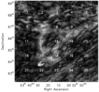
To obtain a large field of view, and to reduce off-axis instrumental polarization, the mosaicking technique was used. The telescope cycled through a grid of pointing positions during the 12hr observation, integrating 50 seconds per pointing, so that every pointing position was observed many times per 12hr period. The mosaic was constructed from $5\times 5$ pointings, where the distance between the pointing centers is 1.25°. The edges of the mosaic far away from any pointing center display high instrumental polarization, and these were not used in the analysis.

The data were reduced with the newstar reduction package, using the unpolarized calibrator sources 3C48, 3C147 and 3C286, and the polarized calibrators 3C345 and 3C303. The absolute flux scale at 325 MHz is based on a flux density of 26.93 Jy for 3C286 (Baars et al. 1977). For details on the data reduction procedure, see Haverkorn (2002).

Central position	(l,b) = (137°, 7°)
Size	$\sim$ 7°$\times$7°
Pointings	5$\times$5
Frequencies	341, 349, 355, 360, 375 MHz
Resolution	5.0′$\times$5.0′ cosec $\delta$ = 5.0′$\times$5.5′
Noise	$\sim$ 5 mJy/beam (0.7 K)
Conversion Jy-K	1 mJy/beam = 0.146 K (at 350 MHz)
Minimal	Date	Start time	End time
spacing		(UT)	(UT)
36m	95/12/19	15:12	02:58
48m	95/12/20	14:53	02:53
60m	95/12/27	14:20	02:20
72m	96/01/02	14:02	02:02
84m	95/12/12	16:42	03:25
96m	96/01/08	13:38	01:38

Table 1: Observational details of the Horologium field

To avoid radio interference from the Sun, the observations were taken mostly or completely at night, as shown in Table 1. Because the observations were done in winter, and during a solar minimum, the total electron content (TEC) of the ionosphere is low. These observing conditions minimize the ionospheric Faraday rotation. We can estimate the $RM$ contribution of the ionosphere from the TEC of the ionosphere and the earth magnetic field. The TEC of the ionosphere above Westerbork at night, in a solar minimum, and in winter is minimal: TEC $\approx 2.2\;10^{16}$ electrons cm^-2 (Campbell, private communication). Assuming a vertical component of the earth magnetic field of 4.5 G down wards, and a path length through the ionosphere of 300 km, the $RM$ caused by the ionosphere is –0.25 rad m^-2 at hour angle zero. At larger hour angles, this is even less. So we expect the rotation measure values given in this paper not to be affected by ionospheric Faraday rotation by more than 0.5 rad m^-2.

2.1 Missing large scale structure

An interferometer is insensitive to structure on large angular scales due to missing short spacings. The smallest baseline attainable with the WSRT of 36m means that scales above approximately a degree are attenuated sufficiently as to be undetectable. The $Q$ and $U$ maps are constructed so that in each mosaic pointing, the map integrals of $Q$ and $U$ are zero. This leads to missing large-scale components in $Q$ and $U$, and therefore erroneous determinations of $P$, $\phi$ and $RM$. However, if the variation in $RM$ is large enough within one pointing, the variation in polarization angle is so large that the average $Q$ and $U$ are close to zero. In this case, missing large-scale components are negligible.

In the field of observation discussed here, $\sigma_{\scriptscriptstyle\rm RM}$ $>1.8$ rad m^-2 in most pointings, which means that in these pointings missing large-scale components cannot account to more than a few percent of the small-scale signal. The 25 pointing centers are shown in Fig. 1. In four pointings $\sigma_{\scriptscriptstyle\rm RM}$ $\la 1.8$ rad m^-2, which means that offsets could amount to 15 - 30% of the signal. These pointings are numbers 9, 10, 12 and 24, and the $\sigma_{\scriptscriptstyle\rm RM}$ in those pointings are $\sim$ 1.6, $\sim$ 1.7, $\sim$ 1.7 and $\sim$ 1.3 respectively. All $\sigma_{\scriptscriptstyle\rm RM}$ are computed only at positions where $\langle P\rangle>20$ mJy/beam and reduced $\chi^{2}$ of the linear $\phi(\lambda^{2})$-relation $\chi^{2}_{red}<2$ (see Sect. 3.5). So, care must be exercised in interpreting the polarization data from these pointing centers. On the other hand, polarization angles show a linear variation over frequency in a large part of the data, yielding good $RM$ determinations, which would not be possible if large-scale offsets dominate. See Haverkorn et al. (2003a) for an extended discussion of this point.

Figure 1: Individual pointings are numbered 1 to 25, superimposed on polarized intensity at 349 MHz.

3 Observational results

3.1 Stokes $Q$ and $U$

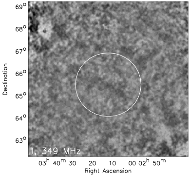
Figure 2: Stokes Q (left) and U (right) at 349 MHz, with a resolution of about 5′. A circle with radius 1.44° and centered on $(\alpha,\delta)=(48.05\degr,65.73\degr)$ is superimposed.

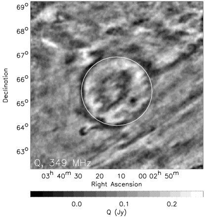
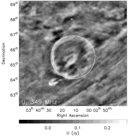
The observed Stokes $Q$ and $U$ intensities at the 5′ resolution are shown in Fig. 2. The distributions of $Q$ and $U$ values in the field are approximately Gaussian, centered around zero, and have a width of 20 to 25 mJy/beam (equivalent to polarized brightness temperatures $T_{b,pol}$ of 2.9 - 3.7 K) for the five frequencies. The ring structure is clearly visible in $Q$ and $U$. To emphasize the perfect circularity of the ring, a circle of radius 1.44° and centered on $(\alpha,\delta)=(48.05\degr,65.73\degr)$, which was fitted by eye to the ring-like structure in $Q$ and $U$, is superimposed in both maps.

3.2 Polarized intensity $P$

Figure 3: Polarized intensity $P$ for each frequency, at 5′ resolution, and total intensity $I$ in the lower right plot. Superimposed are lines of constant Galactic latitude, and the same circle as in Fig. 2.

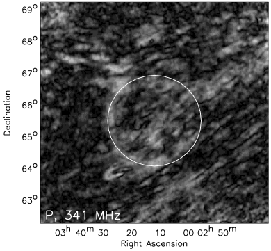
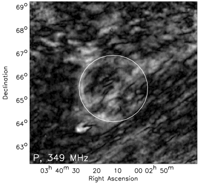
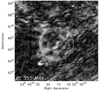
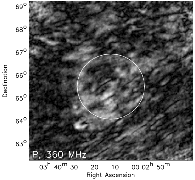
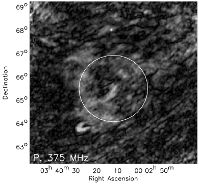
The maps of polarized intensity $P$ derived from the Stokes $Q$ and $U$ maps are shown in Fig. 3 for all 5 frequencies. White denotes the highest intensity, and intensities above 110 mJy/beam (equal to $T_{b,pol}=16$ K) are saturated. The maximum intensities in the 5 frequency bands are 141, 122, 107, 120, and 143 mJy/beam, respectively. Superimposed are lines of constant Galactic latitude $b=$3°, 5°, 7°, 9°, and 11°, and the superimposed circle is the same as the one in Fig. 2. Several regions of different topology of polarized intensity are present in the field:

1. The most conspicuous feature is the ring in the center of the field. Although it is not as distinct as in polarization angle and Stokes $Q$ and $U$, the ring is still clearly visible in $P$ over most of its circumference. Only in the southwest, the ring is not well defined. At 375 MHz, the ring seems to be more blurred than at the other frequencies.

2. A linear structure of high polarized intensity extends from the center of the ring towards the northwest, and is approximately aligned with Galactic latitude. We discuss this elongated structure of high $P$ in Sect. 8.1.

3. The southwestern corner of the field shows a filamentary pattern of “canals” of low $P$ running from southeast to northwest, approximately along lines of constant Galactic latitude, that are remarkably straight over many degrees and always one beam width wide. This pattern is also visible in angle (Fig. 4) and Stokes $Q$ and $U$ (Fig. 2). The southwestern part of the ring appears deformed in the direction of the filaments, but this deformation can be caused by averaging over the line of sight, so that the ring and filaments are not necessarily located at the same distance. Across the canals, there is an angle difference of 90° (or 270°, 450° etc.).

3.3 Total intensity $I$

In the lower right plot of Fig. 3 a map of total intensity $I$ at 349 MHz is shown, from which point sources $>5$ mJy/beam are removed. The map has the same resolution of 5.0′$\times$5.5′ and the same brightness scaling as the $P$ maps in the other panels of the same figure.

No structure in total intensity $I$ is visible, although there is abundant structure in polarization. The circular structure in the upper left corner of the $I$ map is artificial and caused by a very bright unpolarized extragalactic source at that position. As an interferometer acts as a high-pass filter, the map integral $I$ over the field is set to zero by lack of information about its true level. From the single dish survey of Haslam et al. (1981, 1982) at 408 MHz, the total brightness temperature at 408 MHz at this position is approximately 44.5 K with a temperature uncertainty of $\sim$ 10% and including 2.7 K from the cosmic microwave background. To obtain the brightness temperature of the diffuse emission at 350 MHz, the contribution of 2.7 K from the CMBR is subtracted, as well as the contribution of 25% from discrete sources, derived from source counts (Bridle et al. 1972), assuming the spectral index of the Galactic background and the extragalactic sources to be identical. The intensities from the Haslam survey were scaled to our frequencies with a temperature spectral index of $-$2.7. We thus estimate the total brightness temperature at $\sim$ 350 MHz to be 47 K. The apparent degree of polarization $p$ ($=P/I$) is mostly above 100%. This indicates that $I$ is uniform on the scales that the WSRT is sensitive to, and therefore the measured $I$ is close to zero. Small-scale structure in polarization due to Faraday rotation and depolarization causes higher $P$ than $I$, resulting in $p>100$%.

3.4 Polarization angle

Figure 4: Polarization angle in the Horologium field at 349 MHz. The grey scale runs from $-90\degr$ to 90°, so that white is equivalent to black. The superimposed circle is the same as in Fig. 2.

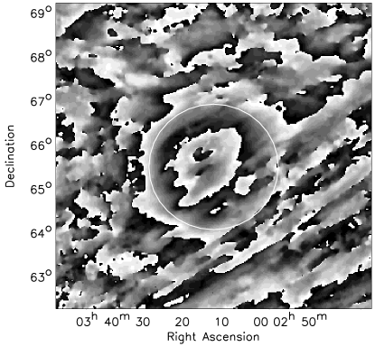
In Fig. 4 we show a grey scale plot of polarization angle in the Horologium region at 349 MHz. The range in angle is [–90°, 90°], so that white denotes the same angle as black. The ring-like structure is well visible, and is close to circular everywhere except on the southwestern side.

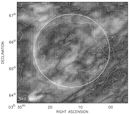
The variation of polarization angle across the ring is shown in Fig. 5, where the grey scale is $P$ at a frequency of 349 MHz and the polarization (pseudo-)vectors are superimposed. The length of the vectors is proportional to $P$. The superimposed contours are contours of polarization angle, and the circle is the same circle as in Fig. 2. The polarization angle is almost perfectly constant over the surface of the ring, and only disturbed in the southwest.

3.5 Rotation measure

Rotation measures were calculated by linearly fitting the observed polarization angle $\phi$ as a function of $\lambda^{2}$. The polarization vectors have an $n180\degr$ ambiguity, but the derived rotation measures are so small that this ambiguity does not play a rôle in our observations: $|RM|\la 10$ rad m^-2, which means an angle change over the full frequency range of 341 MHz to 375 MHz $\Delta\phi\la 75\degr$. Therefore, we calculate the $RM$ values straightforwardly with angle differences minimized.

Figure 5: Detail of the Horologium field, where superimposed vectors are polarization vectors, and the grey scale is polarized intensity at 349 MHz. The superimposed circle is the same as in Fig. 2. The contours delineate also polarization angle, showing that polarization angle is constant over the ring, except for the perturbation in the southwestern corner.

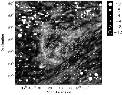
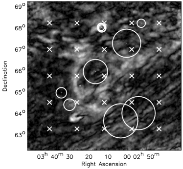
There are various mechanisms that can destroy the linear relation between $\phi$ and $\lambda^{2}$ and make $RM$ determination unreliable, such as depolarization (see Sect. 5) and the insensitivity to large-scale structure (see Sect. 2.1). We have only taken into account those $RM$ values for which the linear $\phi(\lambda^{2})$-relation has reduced $\chi^{2}<2$ and where the polarized intensity averaged over all wavelengths $\left<P\right>>20$ mJy/beam ($\sim$ 4 $\sigma$). About 62% of the polarized intensity data has $\left<P\right>>20$ mJy/beam, and approximately 29% of these data (i.e. $\sim$ 18% of he total) also has a reduced $\chi^{2}<2$. The resulting $RM$ map is given in Fig. 6. The circles denote valid $RM$ values according to the above definition, where the diameter of the circle is proportional to the magnitude of the $RM$. Filled circles denote positive rotation measures. For clarity, only one out of two independent beams in both directions is shown.

In the area enclosed by the ring all the $RM$s are negative, decreasing towards the center of the ring to $RM\approx-8$ rad m^-2. Further away from the center of the ring, $RM$s increase up to a positive $RM$ of a few rad m^-2 at the edges of the field. These values are in agreement with earlier measurements at lower resolution. In rotation measure maps produced by Bingham & Shakeshaft (1967) and by Spoelstra (1984), $|RM|\la 3$ rad m^-2 outside the ring. They presented values of $RM$ inside the ring of $RM<-5$ rad m^-2 and $RM<-3$ rad m^-2, respectively.

Figure 6: Rotation measure map. Circles represent $RM$s for which reduced $\chi^{2}<2$ and $\left<P\right>>20$ mJy/beam $\approx 4\sigma$. The diameters of the circles scale with $RM$, and positive $RM$s are denoted by filled circles. Only one in four beams is shown.

3.6 Extragalactic sources

Figure 7: Graphs of polarization angle $\phi$ against $\lambda^{2}$ for the 12 polarized extragalactic sources in the field. Note that the scaling on the $y$-axis is different for each plot.

Twelve polarized extragalactic sources were detected in the field. The properties of the extragalactic sources were measured in maps with a resolution of 1′. All selected sources have a polarized intensity greater than 4 mJy/beam in each frequency band (the noise in the 1′ resolution data is about 1 mJy/beam) and a degree of polarization greater than 1%. Near the outer edge of the outermost pointing centers, instrumental polarization increases considerably, and sources in that region were excluded. The characteristics of the polarized extragalactic sources are shown in Table 2, the $\phi(\lambda^{2})$-fits in Fig. 7, and the positions of the sources in Fig. 8.

The brightest polarized source in the field with high polarization is the giant double lobed radio galaxy WNB 0313+683 at $(\alpha,\delta)=(3^{h}13^{m},68\degr 20^{m})$ (Schoenmakers et al. 1998). In our analysis this extended source was detected in four separate maxima, viz. sources 5, 6, 7, and 8, all located at approximately the same position in Fig. 8. The high resolution measurements of Schoenmakers et al. (15′′ in the $RM$ map) show an average $RM$ = $-$10.64 rad m^-2, which they argue is Galactic, and a residual $RM$ of about 2 rad m^-2 in each of the lobes. In our 1′ resolution observations at 350 MHz, this would result in a variation in polarization angle within the beam. Depolarization due to this variation in polarization angle can destroy the linear relation between $\phi$ and $\lambda^{2}$ and result in the relatively high $\chi^{2}$ values in sources 5 and 8.

Source no. 3 is the only source with a positive $RM$, which is derived from a good fit with $\chi_{red}^{2}=0.84$. As a check, taking into account the $n\,180\degr$ ambiguity could not yield a $RM$ value closer to that of the other sources. The next best fit has $\chi_{red}^{2}=220$, so $RM$ = 1.6 rad m^-2 is indeed the only acceptable $RM$ determination for this source.

Figure 8: Rotation measures of polarized extragalactic sources indicated by white circles, overlaid on a grey scale representation of polarized intensity at 349 MHz. The $RM$ scales with the diameter of the circles, where the extrema are $-52.6$ rad m^-2 and 1.6 rad m^-2, and open circles denote negative $RM$. Instrumental polarization increases rapidly beyond the outermost pointing centers, denoted by crosses.

Table 2: Polarization data for extragalactic sources with measured polarization in the Horologium field. The second column gives position in $(h\!:\!m,\degr\!:\!m)$, and the third $RM$s with errors. Reduced $\chi^{2}$ of the $\phi(\lambda^{2})$-relation is given in column 4. Columns 5, 6 and 7 give resp. $P$, $I$ (both in mJy/beam) and degree of polarization $p$ in percents, averaged over the five frequency bands.

$$\begin{array}[]{rcr@{\,\,\pm\,\,}lrrrr}\hline\cr\vskip 3.0pt plus 1.0pt minus 1.0pt\cr\mbox{No.}&(\alpha,\delta)&\lx@intercol\hfil RM\;\mbox{(rad\leavevmode\nobreak\ m${}^{-2}$)}\hfil\lx@intercol&\lx@intercol\hfil\;\;\;\chi^{2}\hfil\lx@intercol&\lx@intercol\hfil\;\;\left<P\right>\hfil\lx@intercol&\lx@intercol\hfil\;\;\left<I\right>\hfil\lx@intercol&\lx@intercol\hfil\;\;\left<p\right>\hfil\lx@intercol\\ \vskip 3.0pt plus 1.0pt minus 1.0pt\cr\hline\cr\vskip 3.0pt plus 1.0pt minus 1.0pt\cr 1&\mbox{[3:31,\,65:12]}&\;\;-16.2&1.2&0.37&4.8&168&\;\;2.9\\ 2&\mbox{[3:28,\,64:38]}&\;\;-17.8&1.2&0.67&4.5&253&\;\;1.8\\ 3&\mbox{[3:23,\,65:32]}&\;\;1.6&0.6&0.84&8.7&97&\;\;9.0\\ 4&\mbox{[3:16,\,66:12]}&\;\;-37.4&1.2&1.67&4.4&73&\;\;6.0\\ 5&\mbox{[3:13,\,68:19]}&\;\;-11.5&0.3&3.55&15.5&84&\;\;19.2\\ 6&\mbox{[3:13,\,68:17]}&\;\;-9.1&0.5&0.47&10.4&88&\;\;12.1\\ 7&\mbox{[3:13,\,68:16]}&\;\;-13.3&0.4&1.61&10.6&72&\;\;15.0\\ 8&\mbox{[3:13,\,68:15]}&\;\;-10.8&0.1&13.34&37.3&366&\;\;10.1\\ 9&\mbox{[3:05,\,63:53]}&\;\;-52.6&1.2&0.65&4.4&82&\;\;5.3\\ 10&\mbox{[3:02,\,67:32]}&\;\;-43.5&0.9&1.05&6.4&218&\;\;2.9\\ 11&\mbox{[2:57,\,64:15]}&\;\;-51.1&0.8&1.53&5.6&564&\;\;1.0\\ 12&\mbox{[2:56,\,68:29]}&\;\;-12.8&1.1&1.56&5.5&238&\;\;2.3\\ \vskip 3.0pt plus 1.0pt minus 1.0pt\cr\hline\cr\end{array}$$

4 Observed properties of the ring-like structure

The northeastern half of the ring is very regular in polarized intensity, polarization angle and $RM$, whereas the southwestern part appears to be influenced by the linear structure aligned with Galactic latitude. Therefore, in analyzing the ring structure, we study azimuthal averages of $P$, $\phi$ and $RM$ over position angles (N through E) $-20\degr<\theta<135$°, i.e. the undisturbed part of the ring. The azimuthal averages are centered on $(\alpha,\delta)=(3^{h}12.2^{m},65\degr 44^{m})$, which is the center of the ring superimposed in Fig. 2.

Figure 9: Azimuthal averages of polarized intensity $P$ and total intensity $I$ in Jy/beam for five frequencies (top), polarization angle $\phi$ in degrees for five frequencies (center) and $RM$ (bottom), averaged over the northern and eastern part of the ring structure (position angle $-20\degr<\theta<135$°).

In Fig. 9, we show the azimuthal averages of $I$, $P$, $RM$ and $\phi$. The top panel shows $P$ and $I$ at 5 frequencies. The peak in $P$ at a radius of about 1.4° coincides with the position of the ring. The polarized brightness temperature $T_{b,pol}$ at that radius is approximately 8 K, $T_{b,pol}$ inside the ring is about 3.8 K, and outside the ring about 3 K. The total intensity $I$ is completely uncorrelated with $P$, and hardly exceeds the noise. Note that the position and width of the peak in $P$ is frequency-independent, while inside the ring the $P$ distribution does vary with frequency.

The middle panel in Fig. 9 shows the weighted azimuthal average of the polarization angle plotted as a function of radius, again at 5 frequencies. The angles in each bin were chosen as close as possible ($\pm$ n180°) to the mean angle value of the bin. Then, the mean value was recalculated and the procedure was repeated until the mean angle converged to a single value. The error bars indicate standard deviations of the angle distribution, given for independent beams only in the 341 MHz frequency band. The angle gradient is remarkably linear between a radius of 0.6° and 1.7°, with some structure at a radius of $\sim$ 1°. Whereas $P$ has a maximum at $\sim$ 1.4°, the linear increase of polarization angle with radius continues to at least 1.7°. This indicates that the structure or feature responsible for the ring in $P$ may be actually larger than the apparent size of the ring.

The bottom panel gives the azimuthally averaged observed $RM$ (only values with $\chi_{red}^{2}<2$ and $\left<P\right>>20$ mJy/beam) and the standard deviations of the distribution of $RM$ over each interval. The $RM$ does not vary much over the region at which the peak in $P$ occurs. At radii larger than 1.7°, the $RM$ is slightly positive: $0\la RM\la 2$ rad m^-2. At smaller radii, $RM$ is negative, decreasing to $RM\approx-8$ rad m^-2 in the center, with a small increase around a radius $r=0.7$°. This disk of negative $RM$ in an environment of positive $RM$ is also observed in earlier studies (Bingham & Shakeshaft 1967, Spoelstra 1984). Although the general shape of the $RM$ curve corresponds well to the shape of the polarization angle curve, the shapes are different in detail, which we attribute to an imperfect linear relation between $\phi$ and $\lambda^{2}$.

The observations in $I$, $P$, $\phi$ and $RM$ impose stringent constraints on the nature of the ring. The distribution of $RM$ provides the strongest constraint: $RM$ is positive outside the ring, negative inside and the most negative at the center. The positive $RM$ at large radii from the center of the ring is not necessarily connected to the ring, but could also denote a background magnetic field, of which the parallel component is directed towards the observer. Although $RM$ structure is created by a combination of structure in thermal electron density and magnetic field, a change in sign of $RM$ always indicates a reversal of the parallel component of the magnetic field. So the magnetic field configuration that causes the ring must reverse direction from outside to inside the ring, and the magnetic field and/or electron density has to be the highest at the center. Furthermore, the lack of correlated $I$-structure implies that the ring in $P$ cannot have been produced by emission. In the next section, we first discuss what processes can cause the observed distributions of $P$, $\phi$ and $RM$ in the ring. Subsequently, we shall describe in Sect. 6 some known structures and objects in the ISM, and discuss whether these are related to the ring structure.

5 The nature of the ring in $P$, $\phi$ and $RM$

From comparison of the $I$ and $P$ maps in Fig. 9, it is clear that the structure in $P$ cannot, even in part, be caused by structure in $I$. Structure in $P$ can also be created by missing large-scale structure in $Q$ and/or $U$, but in Sect. 2.1 we have shown that in these observations missing large-scale structure cannot dominate. Therefore, the ring in $P$ is most likely due to a lack of depolarization. Several depolarization mechanisms can contribute to create the ring in $P$. We shall discuss briefly the different depolarization mechanisms thought to be of importance (for details see Haverkorn et al. 2003a,b).

5.1 Depth depolarization

Figure 10: Azimuthally averaged $P$ (left), $\phi$ (center) and $RM$ (right) plotted as a function of radius for a simple power law decrease of the $B$ and $n_{e}$ distributions. The different lines refer to the 5 frequencies.

Depth depolarization is defined as all depolarization processes occurring along the line of sight and can be due to different physical processes. First, if the magnetic field in a synchrotron emitting medium has small-scale structure, then the emitted (intrinsic) polarization angle of the synchrotron radiation will vary along the line of sight, causing wavelength independent depolarization. Secondly, if the medium also contains thermal electrons, the polarization angle of the radiation will be modulated by Faraday rotation as well, which causes additional depolarization (internal Faraday dispersion). So small-scale structure in (parallel) magnetic field and/or thermal electron density within the synchrotron emitting medium causes small-scale depolarization. These processes were described analytically by Sokoloff et al. (1998) for several different geometries of the medium, and numerically in Haverkorn et al. (2003b) using observational constraints.

We modeled the effect of depth depolarization in the observations of the ring-structure using simple distributions of electron density $n_{e}$ and magnetic field $B$ on a rectangular grid. These distributions are not self-consistent, but the only goal of this simple model is to obtain a $P$ and $\phi$ distribution that is similar to the observations, i.e. approximately linear in $\phi$ and ring-like in $P$. Synchrotron radiation of emissivity $\varepsilon\propto B_{\perp}^{2}$ is emitted in the regions where $B_{\perp}$ is non-zero, and is Faraday-rotated while propagating through the medium, depending on the local $B_{\parallel}$ and $n_{e}$ distributions. Furthermore, a polarized background contribution $P_{b}$ is added, which is also Faraday-rotated. Both magnetic field components, parallel and perpendicular to the line of sight, and the electron density distribution were assumed to decrease as a power law outwards. The specific values of the power law indices were chosen so that the observed $\phi$ and $RM$ distributions were approximately reproduced (Fig. 10), i.e. the magnetic field decreases as $r^{-5}$ (only at $r>r_{0}$, where $r_{0}$ is a free parameter too) and the electron density decreases as $r^{-0.4}$.

This figure shows the model output $P$ and $\phi$ at 5 frequencies, and $RM$. We have chosen $B_{\parallel}=-3.5\leavevmode\nobreak\ \mu$G, $B_{\perp}=-2\leavevmode\nobreak\ \mu$G, $n_{e}=0.2$ cm^-3, and $P_{b}=4$ K. This reproduces the shape and magnitude of $\phi$ and $RM$ reasonably well, but the $P$ distribution is very different from the observed one. First, the predicted $P$ at the center is much larger than is observed. However, this discrepancy could be explained by assuming a chaotic magnetic field component at the center of the circle (without worrying yet what this could mean physically). This would result in depolarization and a lower observed $P$ in the center of the modeled circle.

However, a more severe problem is posed by the wavelength dependence of the model predictions. Although our models have very different $B$ and $n_{e}$ distributions and either spherical or cylindrical symmetry, they all show a distinct wavelength dependence of the peak in $P$, as in Fig. 10. But from the observations, the position of the peak in $P$ does not change with wavelength, see Fig. 9. The wavelength dependence of $P$ appears to be a generic property of all models involving depolarization due to depth depolarization. However, the mechanism that can create wavelength independent depolarization, viz. tangled magnetic fields, yields structure in $I$, contrary to what is observed. Therefore we conclude that depth depolarization cannot be the main process that creates the ring in $P$, although we do expect depth depolarization to be present, e.g. in depolarizing the background.

5.2 Beam depolarization

Beam depolarization, i.e. the averaging out of polarization vectors within one synthesized beam, is significant in the field. As there is structure in $RM$ on beam scales, it is likely that $RM$ varies on scales smaller than the beam as well. Furthermore, at the positions of the depolarization canals, the influence of beam depolarization is clearly visible, see Sect. 8.3. (Partial) beam depolarization can destroy the linear $\phi(\lambda^{2})$-relation, but does not necessarily do so. At low polarized intensities, the influence of beam depolarization can be considerable, and observed $RM$ values at low polarized intensity should be used with care, as they can deviate from the true $RM$ value.

Beam depolarization, due to chaotic structure in polarization angle on scales smaller than the beam, can arise due to tangled magnetic fields and/or small-scale variations in thermal electron density. A possible explanation for the lack of $P$ in the central part of the ring could be a chaotic magnetic field in the center, while the outer parts of the ring must exhibit very coherent magnetic fields and electron density. However, although $P$ drops towards the center of the ring, polarization angles are coherent over the whole structure, indicating that beam depolarization due to chaotic sub-beam-scale structure does not dominate.

Beam depolarization can also be due to a spatial gradient in $RM$. For a gradient $dRM/dr$ over many beams, the depolarization factor $p$ is (Gaensler et al. 2001)

$$p=\frac{P_{\scriptstyle\rm observed}}{P_{\scriptstyle\rm original}}=\,\exp\left[-\frac{1}{\ln 2}\left(\frac{dRM}{dr}\right)^{2}\lambda^{4}\right]$$ (1)

where $dRM/dr$ is the gradient of $RM$ over the beam and $r$ is the radius of the ring, expressed in the number of beams. In the upper panel of Fig. 11, we compare the observed radial gradient in $RM$ (solid line) with the theoretical $RM$ gradient from Eq. (1) (dotted line), using the observed polarized intensity $P$ at 341 MHz. Using $P$ from other frequency bands gives very similar results. The derivative of the observed $RM$ was computed after smoothing $RM$ by about 1.5 beams (lower panel). At the position of the ring, the modeled $RM$ gradient shows the same decrease as the observed gradient. Furthermore, at the position where the gradient in $RM$ increases, the depolarization also increases. This indicates that the high $P$ within the ring, as well as the decrease in $P$ at the inner and outer boundaries, can be caused by the gradient in $RM$. However, in the center of the ring, as well as outside the ring, the existence of a gradient in $RM$ would result in a lower depolarization than is observed. So both at the center and outside the ring, other depolarization mechanisms contribute significantly.

Figure 11: Top plot: derivative of azimuthally averaged $RM$ with respect to radius $r$. The solid line denotes the observed $dRM/dr$, and the dotted line is $dRM/dr$ derived from the observed polarized intensity, using Eq. (1). Bottom plot: observed azimuthally averaged $RM$ in dots. The superimposed line is the $RM$ smoothed over about 1.5 beams which is used for the estimate of $dRM/dr$.

5.3 The nature of the ring

The distance to the ring-like structure is not constrained. Depth and beam depolarization introduce a Faraday depth or polarization horizon, because polarized radiation emitted at large distances is more likely to be depolarized than radiation emitted nearby. But because the foreground and background of the ring must be very uniform, the polarization horizon can be at very large distances. However, if the ring is located at large distances, say in or behind the Perseus arm, it would require a path length of more than 2 kpc with an unusually uniform magnetic field and electron density along the path length. Moreover, if the ring is in the Perseus arm, its size would be $>100$ pc, which is unlikely in view of the regular shape of the ring. Therefore, the ring is unlikely to be located in (or behind) the Perseus arm and is probably an inter-arm feature.

The reversal in the direction of the magnetic field from outside to inside the ring, and the $RM$ that becomes more negative towards the center, provides strong constraints for possible explanations for the ring, because they would not allow magnetic field configurations that have spherical symmetry (such as stellar winds or supernovae). This is because in those configurations, the $RM$ contribution from the front half of the structure compensates the (opposite) $RM$ contribution from the far end (e.g. radial fields in young supernovae, bubbles blown in a regular magnetic field perpendicular to the line of sight). Alternatively, the $RM$ would be higher at the edges of the ring than in the center (e.g. bubbles blown in a regular magnetic field parallel to the line of sight). Instead, the structure that creates the ring-like structure, must have a magnetic field directed away from us, in surroundings where the magnetic field has a small component towards us. Furthermore, the magnetic field strength and/or electron density must increase from the edge towards the center of the ring. These constraints make a connection of the ring with many known classes of objects unlikely. Below we discuss the plausibility that some known gaseous structures in the ISM could be responsible for the polarized ring.

6 Connection of the ring with known ISM objects

In this section, we discuss several known objects in the ISM to which the ring could possibly be connected. We conclude that the observed $RM$ structure makes a connection to any known ISM object unlikely.

Planetary nebula

The circular form of the ring structure suggests it might be due to a planetary nebula (PN). The radio emission from a PN is free-free emission, which is negligible at our low frequencies for any reasonable temperature. However, the ring has an angular diameter more than ten times as big as any other PN observed before. If the PN were 5 pc in size, about the size of the largest ancient PN known (Tweedy & Kwitter 1996), then it would be at a distance of about 100 pc and it is unlikely that it hasn’t been observed before. Furthermore, it is difficult to see how the magnetic field configuration needed to create the ring could be present in a PN. For these reasons we believe it unlikely that the ring structure is a planetary nebula.

Strömgren sphere from HD20336

Close to the projected center of the ring the B2V star HD20336 is located at a distance of 246 $\pm$ 37 pc (Hipparcos Catalogue, Perryman et al. 1997). Verschuur (1968) suggested that the ring could be related to this star. If the ring-structure in $P$ coincides with the Strömgren sphere of HD20336, its radius would be $R_{s}$ = 6 pc. The excitation parameter $U=R_{s}\,n_{e}^{2/3}$ is 2.6 pc cm^-2 for a B2V star (Panagia 1973), which yields an electron density inside the Strömgren sphere of $n_{e}\approx 0.1$ cm^-3. The emission measure $EM=\int n_{e}^{2}\,dl=2\,U^{3}/R_{s}^{2}$ solely from the Strömgren sphere is 0.96 cm^-6 pc ($\sim$ 2 R), which could have been detected in the Northern Sky Survey of the Wisconsin H$\alpha$ Mapper (WHAM, Haffner et al., in prep., Reynolds et al. 1998), but wasn’t (see Fig. 13). In addition, the Strömgren sphere explanation is unlikely because of the high proper motion of the star, viz. 18 mas/yr, which is equivalent to 5° in a Myr. The recombination time $t_{r}\approx(\alpha^{(2)}\,n_{e})^{-1}$, where the recombination coefficient to the second level of the hydrogen atom $\alpha^{(2)}\approx 1.4\times 10^{-13}$. So the recombination time is 8 Myr with $n_{e}=0.1$ cm^-3. Due to the high proper motion of the star, we conclude that a circular Strömgren sphere cannot be maintained. Rather, the structure would be elongated in the opposite direction to the proper motion of the star. In addition, it is difficult to imagine a Strömgren sphere with a sufficiently asymmetric magnetic field structure to explain the observed $RM$, as described above. Hence, the ring is unlikely to be a Strömgren sphere around the star HD20336.

Stellar wind from HD20336

We use the interstellar wind-blown bubble model by Weaver et al. (1977) to estimate the time needed to blow a bubble of radius 6 pc with a stellar wind from a B2V star. Weaver et al. estimate the radius of a blown bubble as

$$R_{s}=26.5\;(L_{36}\,n_{H}^{-1}\,t_{6}^{\,3})^{0.2}\mbox{ pc}$$

where $L_{36}$ is the mechanical energy of the stellar wind in units of 10³⁶ erg s^-1, $n_{H}$ is the original hydrogen particle density before passage of the shell, and $t_{6}$ is the elapsed time in Myrs. Assuming that $L_{mech}=2.5\times 10^{-3}L_{bol}$ (Israel & van Driel 1990), and that the absolute luminosity of a B2V star is $L=3.7L_{\odot}$ (Panagia 1973), then $L_{36}=2.2\times 10^{-4}$ erg s^-1. With $R_{s}=6$ pc and $n_{H}=0.1$ cm^-3, the time needed to blow a bubble of the size of the ring is almost 5 Myr. If $n_{H}$ is ten times lower, $t_{6}$ would still be 2.2 Myr. Compared to the proper motion of the star, the time needed to blow a circular bubble is far too long to produce the observed structure. Therefore, the ring cannot be due to the effect of a stellar wind either.

Supernova remnant

For supernova remnants, a $\Sigma$-D relation exists between brightness and distance. Using the non-detection of signal in $I$ as an upper limit for the emission of the ring structure, the $\Sigma$-D relation of Case & Bhattacharya (1998) would imply a distance larger than 36 kpc if the ring was a SNR. Clearly the ring structure is much too faint in $I$ to be related to a supernova remnant.

Superbubble or chimney

Superbubbles that become chimneys as they blow out material from the spiral arm where they originate, have been observed in H i , not only into the Galactic halo, but also into the inter-arm region in the Galactic plane (McClure-Griffiths et al. 2002). The ring could be such a chimney blown away straight from the Sun. Galactic magnetic field frozen in in the plasma that is blown out can cause the observed high negative $RM$. However, if this is the case, one would expect the magnetic field to be maximal at the edges of the chimney, and a low electron density inside the chimney.

7 The ring as a magnetic structure

It is possible that the ring is created through bending of magnetic field lines. E.g. contraction and motion of a plasma cloud or an analogue to the Parker instability can enhance and reverse magnetic fields. The $RM$ plot in Fig. 9 shows an increase in $RM$ out to a radius of about 3°. If the azimuthal average over $RM$ is taken over 360°, $RM$ still increases slowly to 0 rad m^-2 at $r=3$° and to 2 rad m^-2 at $r=4$°. This behavior is more like a magnetic structure, with decreasing magnetic field over a large radius, than like a structure in thermal electron density which has more or less definite boundaries. We conclude that the ring-like structure in $P$ is most likely a funnel-shaped enhancement of magnetic field, directed straight away from us, possibly related to magnetic flux tubes (Parker 1992, Hanasz & Lesch 1993). A “magnetic anomaly” of a few degrees in size has been found in the direction $\ell\approx$ 92°, $b\approx$ 0° (Clegg et al. 1992, Brown & Taylor 2001) from $RM$s of extragalactic sources. However, $RM$s of extragalactic sources in the direction of the ring do not show a local magnetic field reversal (Fig. 8). Therefore we expect the ring-structure to be more localized or less strong than this magnetic anomaly. The magnetic ring-structure may very well be accompanied by an increase in electron density.

Although the distance and shape of the ring-structure are very uncertain, we can try to give estimates of the necessary magnetic field and electron density changes. An upper limit for the change in $n_{e}$ is given by the non-detection of the ring in the Northern Sky Survey of the Wisconsin H$\alpha$ Mapper (WHAM). The WHAM can detect an H$\alpha$ intensity of 0.05 R (1 R = 1 Rayleigh is equal to a brightness of $10^{6}/4\pi$ photons cm^-2 s^-1 ster^-1, and corresponds to an emission measure $EM$ of about 2 cm^-6 pc for gas with a temperature T = 10000 K). So

$$\Delta(n_{e}^{2}\,dl)=2\,n_{e}\,\Delta n_{e}\,dl<0.1\;\;\Rightarrow\;\;\Delta n_{e}\,dl<0.5$$ (2)

assuming a constant path length over the field and a background $n_{e}=0.1$ cm^-3. The change in $RM$ is

$$\Delta RM = 0.81\,\Delta(n_{e}B_{\parallel}dl)$$ (3)

$$= 0.81(\,n_{e}\,\Delta B_{\parallel}\,dl+\Delta n_{e}\,B_{\parallel}\,dl+\Delta n_{e}\,\Delta B_{\parallel}\,dl)$$

The change in $RM$ from inside to outside the ring is $\Delta RM\approx-8$ rad m^-2, and assuming that the background magnetic field $B_{\parallel}\leq 1\mu$G, combination of Eqs. (2) and (3) yields

$$\Delta B_{\parallel}\,(dl+5)\,\hbox{\hbox to0.0pt{\hbox{\lower 4.0pt\hbox{$\sim$}}\hss} \lower-1.0pt\hbox{$>$}}\,100$$ (4)

If $D$ is the distance to the ring, and $f$ is the axial ratio of the object with its major axis along the line of sight, then $dl=Df\tan(3\degr)$. Estimates of $n_{e}$ and minimum $B_{\parallel}$ for different $D$ and $f$ are given in Table 3.

$D$ (pc)	$f$	$\Delta B_{\parallel}$ ($\mu$G)	$\Delta n_{e}$ (cm-3)	$dl$
100	1	$\sim$ $>$  10	0.1	5
500	1	$\sim$ $>$  3	0.02	25
1000	1	$\sim$ $>$  2	0.01	50
100	5	$\sim$ $>$  3	0.02	25
500	5	$\sim$ $>$  0.8	0.004	125
1000	5	$\sim$ $>$  0.4	0.002	250

Table 3: Estimated values of $\Delta B_{\parallel}$ and $\Delta n_{e}$ between ring structure and background, for different estimates of distance $D$ and axial ratio $f$.

If the ring is located at very large distances (say $\,\hbox{\hbox to0.0pt{\hbox{\lower 4.0pt\hbox{$\sim$}}\hss} \lower-1.0pt\hbox{$>$}}\,500$ pc), its width becomes so large that the regularity of the ring becomes hard to explain. A nearby spherical structure ($f=1$) needs a large change in magnetic field, according to Table 3, whereas an elongated structure with a smaller magnetic field change can also accommodate for the observed $RM$ change. In any case, the change in electron density in the ring is small, due to the upper limit imposed by the non-detection of the ring in H$\alpha$.

7.1 Are there more ring-like structures?

	Gray et al. 1998	Uyanıker & Landecker 2002	this paper
$(l,b)$	(137.5°, 1°)	(91.8°, –2.5°)	(137°,7°)
size	1°$\times$2°	(1.5 - 2)°$\times$2°	2.8°$\times$2.8°
$\Delta\phi$	280°	100°	300°
$\Delta RM$	110 rad m-2	40 rad m-2	10 rad m-2
$\phi$ structure	linearly increasing	“linearly” decreasing	linearly decreasing
$P$ structure	ring	ring	ring
distance	440 pc $<d<$ 1.5 kpc	350 $\pm$ 50 pc	?

Table 4: Comparison of the ring discussed here with two earlier detections of circular or elliptical polarization structures by Gray et al. (1998) and Uyanıker & Landecker (2002).

There have been two earlier detections of elliptical structures in polarization angle and polarized intensity without correlated structure in total intensity published, both in single-frequency observations at 1420 MHz. The first detection by Gray et al. (1998) is an elliptical feature of about 2°$\times$1° in size, which shows a linear increase in polarization angle towards the center. Polarized intensity shows a ring-like behavior, and the regular structure in $\phi$ extends to a larger radius than where $P$ peaks.

The “Polarization Lens” observed by Uyanıker & Landecker (2002) shows approximately similar characteristics: an approximately linear decrease of polarization angle towards the center, and a ring-like structure in $P$, although the regular structure in angle seems to trace an ellipse rather than a circle. The characteristics in $P$ and $\phi$ are so similar for the three features, that it is tempting to consider them as members of the same class of objects.

However, although the appearance of the three rings is similar, the changes in $RM$ responsible for the angle changes are vastly different. Although the first two objects are only detected at one frequency, and therefore their $RM$ cannot be determined, a spatial variation in polarization angle is equivalent to a change in $RM$. For the first detection $\Delta RM\approx 110$ rad m^-2, $\Delta RM\approx 40$ rad m^-2 for the second, and $\Delta RM\approx 8$ rad m^-2 for the multi-frequency detection discussed here. If the objects are related, there are two explanations for the differences in $RM$. First, the range in $\Delta RM$ could be due to a difference in magnetic field strength and/or electron density, which would imply that the contraction of magnetic fields and/or enhancement in electron density creating the ring must vary over a large range of scales. Secondly, the range in $\Delta RM$ could be due to a difference in size over which the RM exhibits a linear gradient with equal $\Delta RM$ per parsec for each ring. If we assume a distance for the ring detected by Gray et al. to be 1000 pc, then the first two objects would be consistent with a gradient of $\sim$ 3 rad m^-2 per parsec across the plane of the sky. If our observed ring would be a feature similar to this, the size of the ring would be about 3 pc and its distance 60 pc. In this scenario, rings with similar magnetic field and electron density characteristics would show a range in size (35 pc, 12 pc and 3 pc).

The first two objects were interpreted to be mainly due to an increase of electron density. This explanation cannot apply to the ring discussed here, however, because we observe a change in sign in $RM$ from outside to inside the ring, implying that the cause of the structure must be at least partly magnetic.

The reason that Gray et al. and Uyanıker & Landecker assume that the rings reflect an increase in electron density are the following. First, if the structure was magnetic, the magnetic field enhancement $\Delta B_{\parallel}$ would be $\sim$ 5 times the random component of the magnetic field. This high magnetic field, and a configuration with the magnetic field directed along the line of sight was considered to be very unlikely.

However, in their estimate of the $\Delta B_{\parallel}$ that is necessary to produce the observed $\Delta RM$, they assume that the ring-like structure is an oblate ellipse. If the magnetic field is funnel-shaped instead, the path length through the structure would increase enormously and lower $\Delta B_{\parallel}$ values can account for the observed $\Delta RM$. An alignment with the line of sight seems fortuitous, but it may well be that it is the only configuration that we can observe, because only such a configuration has a long path length through a strong $B_{\parallel}$, making $RM$s dominant over the background.

We conclude that the magnetic field must play an essential rôle in the shaping of the rings, although an increase in electron density is likely to also be of importance. The three detected ring-like structures could be similar objects, although they would need to exhibit a range in magnetic field and electron density, and/or size.

8 Structure outside the ring

8.1 The elongated structure of high $P$

The elongated structure of high $P$ extending from the center of the ring to the northwest can be explained with the scenario sketched by Verschuur (1969). Using the Green Bank 300ft telescope, he observed a filamentary deficit of H i , where the filament starts at the position of the B2V star discussed in Sect. 1, and extends in the direction opposite to the star’s proper motion, along the bar of high $P$ present in our observations. He argues that the star has tunneled through the H i and has blown the neutral material away. Radiation from the star could then have ionized the remaining low density material in the tunnel. This picture is consistent with the filament of high polarization that we see at the same position, from the center of the ring to the northwest.

However, the H i deficit seems to have the same topology as the ring on the eastern edge, i.e. the deficit is shaped as a semi-circle which coincides with the position of the ring. Then, it is probable that the ionization tunnel and the ring structure are at same distance (viz. $\sim$ 250 pc), although they do not necessarily have the same origin.

8.2 Uniform Galactic magnetic field

The coherence in $\phi$, and to a lesser extent in $P$, over a large part of the ring indicates that the polarized foreground and background have to be uniform on the scale of the ring. If structure in $RM$ on smaller scales was present somewhere in the line of sight, be it in front of or behind the ring-like structure, the linearity of angle with radius would be destroyed. Small deviations from linearity are present (see e.g. the patch of less negative $RM$s at $(\alpha,\delta)=(3^{h}18^{m},66\degr)$), which indicates a change in $RM$ of a few rad m^-2 somewhere along the line of sight. However, in general the medium must be very uniform to give such large coherent behavior in the polarization angle as observed in the ring.

The ring is located in the “fan region”, which is a region of high polarization even at low frequencies (Brouw & Spoelstra, 1976) and with very ordered polarization angles, located at about $120\degr\la\ell\la 160\degr$, $0\degr\la b\la 20\degr$. The high polarization in this region indicates less depolarization, and therefore the uniform magnetic field should dominate over the random magnetic field component. From external galaxies, there are indications that indeed the uniform magnetic field component is higher than the random component between the spiral arms (Beck & Hoernes 1996, Beck et al. 1996).

From Fig. 6, and the $RM$ determinations of Spoelstra (1984) and Bingham & Shakeshaft (1967), we derive that outside the ring, $RM$ $\la 6$ rad m^-2. Then, the parallel component of the magnetic field must be $B_{\parallel}\la 0.2\leavevmode\nobreak\ \mu$G, assuming a path length of the polarized radiation of 600 pc (Haverkorn et al. 2003b) and a thermal electron density of 0.08 cm^-3 (Reynolds 1991). The path length is probably longer than 600 pc, which only reduces $B_{\parallel}$ further. This very low value of $B_{\parallel}$ is in agreement with the uniform magnetic field being mostly perpendicular to the line of sight in this direction.

8.3 The aligned depolarization canals

Figure 12: Left: $P$ at 349 MHz where the white box denotes the volume used in the right plot. Right: the symbols denote $RM$ against a coordinate in the approximate direction of Galactic latitude “$b$” (top) and longitude “$\ell$” (bottom), where 1 pixel is $\sim$ 0.6′. $RM$ is averaged over “$\ell$” and “$b$”, respectively. The plotted error in $RM$ is the error in the mean of $RM$ in each bin. The upper line is $P$ at 349 MHz averaged over the same bins.

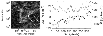
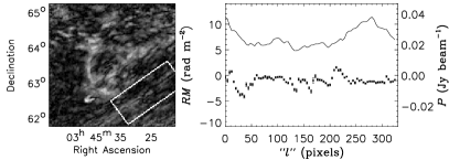
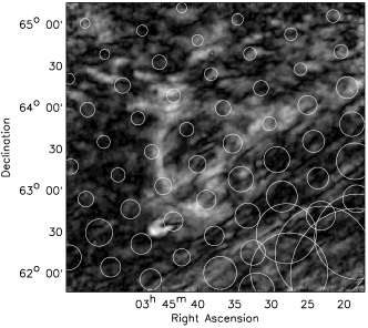
In the southwestern part of the field, long and straight depolarization canals exist that are approximately aligned with Galactic latitude and one synthesized beam wide, see Fig. 3. Fig. 12 shows the distribution of $RM$ and $P$ along and across the depolarization canals, i.e. approximately along Galactic longitude $\ell$ and latitude $b$. The top plot shows the $RM$ distribution as a function of “$b$”, and the bottom plot as a function of “$\ell$”, where the area used is indicated by the white box in the two left-hand figures. $RM$ and $P$ are averaged in the direction perpendicular to “$\ell$” and “$b$”, respectively. The symbols in the right figures denote $RM$, where the error bars give the standard error in the mean of $RM$ in each bin. The upper lines denote the $P$ distribution at 349 MHz, averaged over a bin. The main difference between the two plots is that the $RM$ along the filaments hardly changes, whereas the $RM$ across the filaments shows a gradient and/or stratification.

Figure 13: H$\alpha$ data from the WHAM survey in circles, with a resolution of 1°, overlaid on polarized intensity at 349 MHz in grey scale. The diameters of the circles are proportional to the H$\alpha$ intensity, which ranges from $\sim$ 2.2 R in the upper left corner, to $\sim$ 30 R in the lower right corner.

To investigate whether this $RM$ structure is due to magnetic fields and/or thermal electron density, we can use independent measurements of $n_{e}$, e.g. from H$\alpha$ observations. We use data from the WHAM Northern Sky survey (Haffner et al., in prep., Reynolds et al. 1998), as shown in Fig. 13. The H$\alpha$ intensity integrated over the velocity range $v=-10$ km s^-1 to $v=-50$ km s^-1 increases from $\sim$ 2.2 R to 30 R. This velocity range coincides with distances of 300 pc to 2.3 kpc using the rotation curve of Fich et al. (1989). If the H$\alpha$ increase is generated over a line of sight of 2 kpc, the necessary increase in thermal electron density is only from 0.055 cm^-3 to 0.07 cm^-3. If we take again the path length of the polarized radiation to be 600 pc, the change in $RM$ seen in Fig. 12, viz 7 rad m^-2, can be made with a constant $B_{\parallel}\approx 0.2\leavevmode\nobreak\ \mu$G, which agrees with the estimate made in Sect. 3.5 for the uniform magnetic field component.

Depolarization canals can have two possible causes. The first is beam depolarization, i.e. the canals denote boundaries between regions of different $RM$ so that $\Delta\phi=90\degr$. $RM$ changes with different magnitudes are likely to exist as well, but these do not leave visible traces in $P$. The second cause for canals is depth depolarization. If the emitting and rotating medium is uniform, $P=\sin(2RM\lambda^{2})/(2RM\lambda^{2})$ so that “nulls” of minimum polarization exist at positions where $2RM\lambda^{2}=n\pi$. However, there is no reason why depolarization canals would be one beam wide in this model, and low-$P$ canals only exist for a uniform medium. Furthermore, the second model predicts the position of the canals to shift with wavelength, which is not observed. Therefore we believe that the depolarization canals are predominantly the result of beam depolarization. For an extended discussion of the causes of depolarization canals, see Haverkorn et al. (2000, 2003a).

Figure 14: Spatial variations of $P$ at 5 frequencies (upper plot), $RM$ (central plot) and $\phi$ (lower plot) over a slit of $\sim$ 1.5′ wide, against “$b$”. $RM$ and $\phi$ values are only given where $\chi_{red}^{2}<2$ and $\left<P\right>>20$ mJy/beam.

If the gradient in $RM$ is constant, depolarization canals due to beam depolarization would not be possible. So the $RM$ must increase discontinuously, as is visible in Fig. 12. If $\Delta RM$ over one beam is between 2.1 and 2.5 rad m^-2 (or between 6.3 and 7.5 rad m^-2, etc.), depolarization canals occur. Fig. 14 shows $P$ and $RM$ over a narrow slit ($\sim$ 1.5′) across the canals plotted against $b$, located within the box in Fig. 12. The top panel shows plots for $P$ at all 5 frequencies, oversampled by a factor of 5. The central panel shows $RM$, where $RM$ values are only plotted for beams for which $\chi_{red}^{2}<2$ and $\left<P\right>>20$ mJy/beam. Polarization angle $\phi$ is given in the bottom panel. The two sharpest depolarization canals visible at all frequencies, at pixel numbers 113 and 145 correspond to abrupt changes in $RM$ of about 2 rad m^-2 and angle changes around 90°. Abrupt $RM$ changes with other magnitudes are present as well, but these do not create depolarization canals.

9 Conclusions

The ring-like structure in polarized intensity $P$ with a radius of about 1.4° shows a regular increase in polarization angle from its center out to $\sim$ 1.7°, suggesting that the structure is a disk instead of a ring, and extends to larger radii than the ring in $P$. The rotation measure is slightly positive outside the ring, reverses sign inside the ring and decreases almost continuously to $RM\leavevmode\nobreak\ \approx-8$ rad m^-2 at the center. This property rules out its production by any spherically symmetric structure, such as a supernova remnant or a wind-blown bubble. The $RM$ structure, and the observation that the coherence in angle slowly disappears beyond a radius of $\sim$ 1.7° indicates a magnetic origin for the polarization ring, probably accompanied by an electron density enhancement. We propose that the ring is produced by a predominantly magnetic funnel-like structure, in which the parallel magnetic field strength is maximal at the center and directed away from us. The enhancement in $P$ at radius $\sim$ 1.4° is caused by a lack of depolarization due to the relative constancy of $RM$ at that radius. A filamentary pattern of parallel, narrow depolarization canals indicates structure in $RM$ which is aligned with Galactic longitude. The depolarization canals are probably created by beam depolarization due to abrupt spatial gradients in $RM$.