Early Optical Afterglows from Wind-Type Gamma-Ray Bursts

Abstract

We study prompt optical emission from reverse shocks in the wind-type gamma-ray bursts. The emission is evaluated in both the thick and thin shell regimes. We discuss the angular time delay effect and the post-shock evolution of the fireball ejecta, which determine the decay index of the prompt optical emission and the duration of the radio flare. We discuss distinct emission signatures of the wind environment compared with the constant interstellar medium environment. We also present two recipes for directly constraining the initial Lorentz factor of the fireball using the reverse and forward shock optical afterglow data for the wind case.

1 Introduction

The gamma-ray burst (GRB) afterglow observations are usually explained by a model in which a relativistic fireball shell (ejecta) is expanding into a uniform interstellar medium (ISM). However, there is observational evidence suggesting a link between GRBs and massive stars or star formation (e.g. Mészáros 2001 for a review). An important consequence of a massive star origin for the afterglow is that the fireball shell should be expanding into a pre-burst stellar wind of the progenitor star with a density distribution of $\rho\propto R^{-2}$ (e.g. Chevalier & Li 1999; Mészáros, Rees & Wijers 1998; Dai & Lu 1998). This wind model is discussed to be consistent with some GRB afterglow data (Chevalier & Li 1999, 2000).

It is expected that many early optical afterglows will be discovered soon in the observational campaigns led by HETE-2 and Swift. Long time span (from right after the GRB trigger to a year) observational data will allow us to distinguish differences between the ISM and wind models clearly.

In this paper, we will discuss the optical reverse shock emission for the wind model in detail. The previous study (Chevalier & Li 2000) gave the discussions for the thick shell case, and we will consider both the thin and thick shell cases. We show that the angular time delay effect plays an important role in discussing the light curve decaying phase of the reverse shock emission.

2 The Model

We consider a relativistic shell (fireball ejecta) with an isotropic energy $E$, an initial Lorentz factor $\eta$ and an initial width $\Delta_{0}$ expanding into a surrounding medium with density distribution of $\rho=AR^{-2}$ (wind model). In this paper, Lorentz factors $\gamma$, radii $R$ and widths $\Delta$ are measured in the laboratory frame where the progenitor is at rest. Thermodynamic quantities: mass densities $\rho$ and internal energy $e$ are measured in the fluid comoving frame. The interaction between the shell and the wind is described by two shocks: a forward shock propagating into the wind and a reverse shock propagating into the shell. The shocks accelerate electrons in the shell and wind material, and the electrons emit photons via synchrotron-cyclotron process. For the synchrotron process, the spectrum of each shock emission is described by a broken power law with a peak $F_{\nu,max}\propto N_{e}B\gamma$ and break frequencies: a typical frequency $\nu_{m}\propto B\gamma\gamma_{m}^{2}$ and a cooling frequency $\nu_{c}\propto 1/B^{3}\gamma t^{2}$ (Sari, Piran & Narayan 1998) where $N_{e}$ is the number of electrons accelerated by the shock, $B$ is the magnetic field strength behind the shock, $\gamma$ and $\gamma_{m}$ are the bulk Lorentz factor of the shocked material and the random Lorentz factor of the typical electrons in the shocked material, respectively. Assuming that constant fractions ($\epsilon_{e}$ and $\epsilon_{B}$) of the internal energy $e$ produced by the shock go into the electrons and the magnetic field, we get $\nu_{m}\propto\gamma\rho^{-2}e^{5/2},\nu_{c}\propto\gamma^{-1}e^{-3/2}t^{-2}$ and $F_{\nu,max}\propto N_{e}\gamma e^{1/2}$.

3 Forward Shock

Observations of optical afterglows usually start around several hours after the burst trigger. At such a late time, the shocked wind material forms a relativistic blast wave and carries almost all the energy of the system. Chevalier & Li (1999) gave the characteristics of the forward shock (blast wave) emission as follows,

$$\nu_{m,f}(t) \sim 1.6\times 10^{12}\zeta^{1/2}\epsilon_{e,-1}^{2}\epsilon_{B,-2}^{1/2}E_{52}^{1/2}t_{d}^{-3/2}~{}\mbox{Hz},$$ (1)

$$\nu_{c,f}(t) \sim 6.3\times 10^{13}\zeta^{-3/2}\epsilon_{B,-2}^{-3/2}E_{52}^{1/2}A_{\ast}^{-2}t_{d}^{1/2}~{}\mbox{Hz},$$ (2)

$$F_{\nu,max,f}(t) \sim 4.5~{}d^{-2}\zeta^{3/2}\epsilon_{B,-2}^{1/2}E_{52}^{1/2}A_{\ast}t_{d}^{-1/2}~{}\mbox{mJy},$$ (3)

where $\zeta=(1+z)/2$, $d=d_{L}(z)/(2\times 10^{28}$cm), $z$ and $d_{L}(z)$ are the redshift and luminosity distance of the burst, respectively, $d_{L}(1)\sim 2\times 10^{28}$cm for the standard cosmological parameters ($\Omega_{m}=0.3$, $\Omega_{\Lambda}=0.7$ and $h=0.7$), $\epsilon_{e,-1}=\epsilon_{e}/0.1$, $\epsilon_{B,-2}=\epsilon_{B}/0.01$, $E_{52}=E/10^{52}$ ergs, $A_{\ast}=A/5\times 10^{11}$ g cm^-1, $t_{d}$ is the observer’s time in units of days. The optical flux from the forward shock decays proportional to $t^{-1/4}$ initially, and decays faster as $t^{-(3p-2)/4}$ after a transition of $\nu_{m,f}$ through the optical band $\nu_{R}\sim 5\times 10^{14}$Hz (Chevalier & Li 2000) where $p$ is the index of the power law distribution of the accelerated electrons. Using $\nu_{R\ast}=\nu_{R}/5\times 10^{14}$Hz, the break time $t_{m,f}$ (the passage of $\nu_{m,f}$) and the optical flux (in the fast-cooling regime) at that time are

$$t_{m,f} \sim 30~{}\zeta^{1/3}\epsilon_{e,-1}^{4/3}\epsilon_{B,-2}^{1/3}E_{52}^{1/3}\nu_{R\ast}^{-2/3}~{}\mbox{min},$$ (4)

$$F_{\nu_{R},f}(t_{m,f}) \sim 4~{}d^{-2}\zeta^{2/3}\epsilon_{e,-1}^{-1/3}\epsilon_{B,-2}^{-1/3}E_{52}^{2/3}\nu_{R\ast}^{-1/3}~{}\mbox{mJy}.$$ (5)

4 Reverse Shock

At earlier time when the reverse shock crosses the shell, the forward-shocked wind and the reverse shocked shell carry comparable amount of energy. A significant emission is expected from the reverse shock also (Mészáros & Rees 1997; Sari & Piran 1999a). During the reverse shock crossing, there are four regions separated by the two shocks: the wind (denoted by the subscript 1), the shocked wind (2), the shocked shell material (3) and the unshocked shell material (4). Using the jump conditions for the shocks and the equality of pressure and velocity along the contact discontinuity, we can estimate the Lorentz factor $\gamma_{i}$, the internal energy $e_{i}$ and the mass density $\rho_{i}$ in the shocked regions as functions of three variables $\gamma_{4}(=\eta)$, $\rho_{1}$ and $\rho_{4}$ (Sari and Piran 1995).

There are two limits to get a simple analytic solution to the hydrodynamic quantities at a shell radius $R$ (Sari and Piran 1995). If the Lorentz factor is low $\eta^{2}\ll f$ where $f=\rho_{4}/\rho_{1}$, the reverse shock is Newtonian which means that the Lorentz factor of the shocked shell material is almost unity in the frame of the unshocked shell material. It is too weak to slow down the shell effectively so that $\gamma_{3}\sim\eta$. On the other hand, if the Lorentz factor is high $\eta^{2}\gg f$, the reverse shock is relativistic, and considerably decelerates the shell material, hence $\gamma_{3}\sim\eta^{1/2}f^{1/4}$.

4.1 Critical Radii

Since the density ratio $f$ is generally a function of $R$, there is a possibility that the reverse shock evolves from Newtonian to relativistic during the propagation. The evolution of the reverse shock depends on the ratio of two radii: $R_{\gamma}\equiv E/4\pi Ac^{2}\eta^{2}$ where the forward shock sweeps a mass of $E/c^{2}\eta^{2}$ and $R_{s}\equiv\Delta_{0}\eta^{2}$ where the shell begins to spread if the initial Lorentz factor varies by order $\eta$ (Sari & Piran 1995; Kobayashi, Piran & Sari 1999). Another important radius is $R_{\times}$ where the reverse shock crosses the shell. The lab-frame time it takes for the reverse shock to cross a width $dx$ of the shell material is given by $dt_{lab}\sim dR/c\sim\eta f^{1/2}dx/c$ (Sari & Piran 1995). We can regard $R/c$ as time $t_{lab}$ in the laboratory frame because of the highly relativistic expansion of the shell. Since the whole shell width is $\Delta\sim\max[\Delta_{0},R/\eta^{2}]$, we obtain $R_{\times}\sim\max[(R_{s}R_{\gamma})^{1/2},R_{\gamma}]$.

Considering $\eta^{2}/f=\max[R_{s}/R_{\gamma},R/R_{\gamma}]$, we can classify the evolution of reverse shocks into two cases by using a critical Lorentz factor $\eta_{c}\equiv(E/4\pi Ac^{2}\Delta_{0})^{1/4}$ (see Sari & Piran 1995 and Kobayashi & Zhang 2003 for the ISM model). If $R_{s}/R_{\gamma}=(\eta/\eta_{c})^{4}>1$ (Thick Shell Case), the reverse shock is relativistic from the beginning (at the end of the GRB phase), which is different from the ISM model in which the reverse shock only becomes relativistic later. The reverse shock crosses the shell at $R_{\times}\sim(R_{s}R_{\gamma})^{1/2}$ before the shell begins to spread at $R_{s}$, and it significantly decelerates the shell material $\gamma_{3}\sim\eta_{c}$. If $R_{s}/R_{\gamma}<1$ (Thin Shell Case), the reverse shock is initially Newtonian and becomes only mildly relativistic when it traverses the shell at $R_{\times}\sim R_{\gamma}$. We can regard $\gamma_{3}$ as constant ($\sim\eta$) during the shock crossing.

4.2 Synchrotron Emission

Since the wind density at the initial interaction is much larger than the medium density for the ISM model, the cooling frequency $\nu_{c,r}$ of the reverse shock emission is much lower than the typical (injection) frequency $\nu_{m,r}$ in the wind model. The random Lorentz factor $\gamma_{c}$ of the electrons that radiate at the cooling frequency $\nu_{c,r}$ could be sub-relativistic or Newtonian, $\gamma_{c}(t_{\times})\sim 1\zeta^{-7/4}\epsilon_{B,-2}^{-1}A_{\ast}^{-5/4}E_{52}^{1/4}t_{\times,\ast}^{3/4}$ for our typical parameters. This makes the radiation mechanism cyclotron radiation at low frequencies $\sim\nu_{c,r}$ and at early times $<t_{\times}$. However, the detailed modelling on the cyclotron emission is not important, because the flux is suppressed and determined by the self absorption. (We will discuss the self-absorption at the end of this subsection.) On the other hand, the random Lorentz factor $\gamma_{\nu_{R}}$ of the electrons corresponding to the optical frequency $\nu_{R}$ is relativistic. Since the electron distribution $N(\gamma_{e})$ around $\gamma_{\nu_{R}}$ (and above it) is determined by the distribution of injected electrons at the shock, which are relativistic, and by the synchrotron radiation cooling, we apply the conventional synchrotron model to estimates the light curve of optical flashes.

The observer time $t\equiv(1+z)R/c\gamma^{2}$ is proportional to $R$, because the Lorentz factor of the shocked shell during the shock crossing $\gamma_{\times}\sim\min[\eta,\eta_{c}]$ is constant. By using the shock jump conditions, one finds that the scalings before the crossing time $t_{\times}=(1+z)R_{\times}/c\gamma_{\times}^{2}$ are given by $e_{3}\propto t^{-2}$, $\rho_{3}\propto t^{-2}$ and $N_{e}\propto t$ in the thick shell case, and $e_{3}\propto t^{-2}$, $\rho_{3}\propto t^{-3}$ and $N_{e}\propto t^{1/2}$ in the thin shell case. The scalings of the spectral characteristics at $t<t_{\times}$ are $\nu_{m,r}\propto t^{-1},\nu_{c,r}\propto t$ and $F_{\nu,max,r}\propto t^{0}$ for thick shell and $\nu_{m,r}\propto\nu_{c,r}\propto t$ and $F_{\nu,max,r}\propto t^{-1/2}$ for thin shell. The scalings of $\nu_{c,r}$ and $F_{\nu,max,r}$ themselves are not correct, but the optical flux estimated by these scalings are right. We evaluated the scalings to calculate the optical light curve.

The initial shell width $\Delta_{0}$ is given by the intrinsic duration of the GRB, $\Delta_{0}\sim(1+z)^{-1}cT$ (Kobayashi, Piran & Sari 1997), the shock crossing time $t_{\times}$ can be written in the following form,

$$t_{\times}\sim\left(\frac{\gamma_{\times}}{\eta_{c}}\right)^{-4}T,$$ (6)

where $\eta_{c}\sim 60~{}\zeta^{1/4}E_{52}^{1/4}A_{\ast}^{-1/4}T_{1}^{-1/4}$ and $T_{1}=T/10$sec. We can determine the critical Lorentz factor $\eta_{c}$ from the observations of the GRB and afterglow. If we detect the shock crossing time $t_{\times}$ (the reverse shock peak time), the Lorentz factor during the shock crossing time $\gamma_{\times}$ can be estimated from eq. (6).

The spectral characteristics of the reverse shock emission at $t_{\times}$ are related to those of the forward shock emission by the following simple formulae (Kobayashi &Zhang 2003),

$$\nu_{m,r}(t_{\times})\sim\frac{\eta^{2}}{\gamma_{\times}^{4}}\nu_{m,f}(t_{\times}),\ \ \ \nu_{c,r}(t_{\times})\sim\nu_{c,f}(t_{\times}),\ \ \ F_{\nu,max,r}(t_{\times})\sim\frac{\gamma_{\times}^{2}}{\eta}F_{\nu,max,f}(t_{\times}).$$ (7)

Using eqs. (1), (2) and (3), we get

$$\nu_{m,r}(t_{\times}) \sim 5.0\times 10^{14}~{}\zeta^{-1/2}\epsilon_{e,-1}^{2}\epsilon_{B,-2}^{1/2}E_{52}^{-1/2}A_{\ast}\eta_{2}^{2}t_{\times,\ast}^{-1/2}~{}\mbox{Hz}$$ (8)

$$\nu_{c,r}(t_{\times}) \sim 1.5\times 10^{12}~{}\zeta^{-3/2}\epsilon_{B,-2}^{-3/2}E_{52}^{1/2}A_{\ast}^{-2}t_{\times,\ast}^{1/2}~{}\mbox{Hz}$$ (9)

$$F_{\nu,max,r}(t_{\times}) \sim 3.0~{}d^{-2}\zeta^{2}\epsilon_{B,-2}^{1/2}E_{52}A_{\ast}^{1/2}\eta_{2}^{-1}t_{\times,\ast}^{-1}~{}\mbox{Jy}$$ (10)

where $\eta_{2}=\eta/100$ and $t_{\times,\ast}=t_{\times}/50$sec. The reverse shock emission is in the fast cooling regime $\nu_{c,r}<\nu_{m,r}$ during the shock crossing. So for $t<t_{\times}$, the optical flux from the reverse shock increases as $\propto t^{1/2}$ for thick shell case ($\nu_{R}<\nu_{m,r}(t_{\times})$) (Chevalier & Li 2000), and $\propto t^{(p-1)/2}$ for thin shell case ($\nu_{R}>\nu_{m,r}(t_{\times})$). Since the Lorentz factor of the forward-shocked material is also constant during shock crossing, the optical emission from the forward shock evolves as $t^{1/2}$ at $t<t_{\times}$. But this component is usually masked by the reverse shock emission.

At the shock crossing time $t_{\times}$, the optical flux reaches the peak $F_{\nu_{R},r}$ $\sim F_{\nu,max,r}$ $(\nu_{R}/\nu_{c,r})^{-1/2}$.

$$F_{\nu_{R},r}(t_{\times})\sim 160~{}d^{-2}\zeta^{5/4}\epsilon_{B,-2}^{-1/4}E_{52}^{5/4}A_{\ast}^{-1/2}\nu_{R\ast}^{-1/2}\eta_{2}^{-1}t_{\times,\ast}^{-3/4}~{}\mbox{mJy}$$ (11)

Generally, using the time dependences of the spectral characteristics as well as eq. (7), we can relate this peak flux with the optical flux of the forward shock at the break time,

$$F_{\nu_{R},r}(t_{\times})\sim\left(\frac{\gamma_{\times}^{2}}{\eta}\right)^{2-a}\left(\frac{t_{\times}}{t_{m,f}}\right)^{(2-3a)/4}F_{\nu_{R},f}(t_{m,f}).$$ (12)

where $a=p$ if $\nu_{m,r}(t_{\times})$ is below the optical band, and $a=1$ if it is above. Detection of the peak $(t_{\times},F_{\nu_{R},r}(t_{\times}))$ and the break $(t_{m,f},F_{\nu_{R},f}(t_{m,f}))$ will give a constraint on the initial Lorentz factor $\eta$. A similar recipe has been proposed by Zhang et al. (2003) for the ISM case.

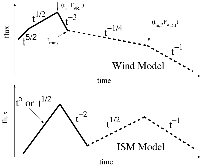
Synchrotron self-absorption would reduce our estimate (11) of the optical flash if it is optically thick. A simple way to account for this effect is to estimate the maximal flux emitted by the shocked shell material as a blackbody (Sari & Piran 1999b; Chevalier & Li 2000). The blackbody flux at the optical band $\nu_{R}$ and at the peak time $t_{\times}$ is given by $F_{\nu_{R},BB}\sim 16~{}\zeta^{5/4}d^{-2}\nu_{R\ast}^{5/2}$ $\epsilon_{B,-2}^{-1/4}A_{\ast}^{-1}E_{52}^{3/4}$ $t_{\times,\ast}^{7/4}$ Jy. The self-absorption frequency at the peak time is $\nu_{sa}\sim 1.0\times 10^{14}A_{\ast}^{1/6}E_{52}^{1/6}\eta_{2}^{-1/3}t_{\times,\ast}^{-5/6}$ Hz. Considering that the peak time $t_{\times}$ is larger than the burst duration $T$, the synchrotron self absorption will not affect the peak flux of an optical flash significantly for long bursts with $T>8~{}\nu_{R\ast}^{-6/5}A_{\ast}^{1/5}E_{52}^{1/5}\eta_{2}^{-2/5}$ sec. However, the self-absorption is important at early times ($<t_{\times}$) in the wind model. The optical light curve should initially behave as $t^{5/2}$ right after the GRB trigger because of the absorption and it turns into $\sim t^{1/2}$ later (see Fig 1). The break time is $t\sim 5~{}\nu_{R\ast}^{-3/2}A_{\ast}^{1/4}E_{52}^{1/4}\eta_{2}^{-1/2}t_{\times,\ast}^{-1/4}$ sec.

4.3 Angular Time Delay Effect

The cooling frequency $\nu_{c,r}(t_{\times})$ is well below the optical band for our typical parameters, the optical emission from the reverse shock should “vanish” after the peak. However, the angular time delay effect prevents abrupt disappearance. The optical light curve at $t>t_{\times}$ is determined by off-axis emissions. In the local frame, the spectral power is described by a broken power law with a low and high frequency indices $-1/2$ and $-p/2$ and the break frequency $\sim\nu_{m,r}(t_{\times})/\gamma_{\times}$. As we see higher latitude emissions, the blue shift effect due to the relativistic expansion becomes smaller. The blue shifted break frequency passes through the optical band $\nu_{R}$ at time $\sim t_{\times}\nu_{m,r}(t_{\times})/\nu_{R}$. The optical flux initially evolves as $t^{-5/2}$ and decays as $t^{-(p+4)/2}$ after the passage (Kumar & Panaitescu 2000b).

Since the forward shock emission decays slower $t^{-1/4}$, it begins to dominate the optical band at $t_{trans}\sim(t_{\times}^{4\alpha}/t_{m,f})^{1/(4\alpha-1)}[F_{\nu_{R},r}(t_{\times})/F_{\nu_{R},f}(t_{m,f})]^{4/(4\alpha-1)}$ where we assumed that the optical reverse shock emission decays proportional to $t^{-\alpha}$. For our typical parameters, $\nu_{m,r}(t_{\times})$ comes to the optical band. Assuming $\alpha=13/4$ (p=2.5) (see fig 1(a) in which $\alpha\sim 3$ is applied), we get $t_{trans}/t_{\times}\sim 2.5~{}\zeta^{1/6}E_{52}^{1/6}A_{\ast}^{-1/6}\eta_{2}^{-1/3}t_{\times,\ast}^{-1/6}$. The optical emission from the reverse shock drops below that from the forward shock within a time scale several times of the peak time $t_{\times}$.

4.4 Duration

If the fireball ejecta is collimated in a jet with an opening angle $\theta_{j}$, the duration of the reverse shock emission is $t_{ang}\sim(1+z)\theta_{j}^{2}R_{\times}/c$. The angle $\theta_{j}$ might be determined from a jet break time $t_{j}\sim(\theta_{j}\gamma_{\times})^{4}t_{\times}$ of the forward shock emission (Rhoads 1999; Sari,Piran & Halpern 1999), even though a jet break in the wind model may not be as clear as that in the ISM model (Kumar & Panaitescu 2000a; Gou et al. 2001).

$$t_{ang}\sim\left(t_{\times}t_{j}\right)^{1/2}\sim 35~{}\left(\frac{t_{\times}}{\mbox{50 sec}}\right)^{1/2}\left(\frac{t_{j}}{\mbox{1 day}}\right)^{1/2}~{}\mbox{min}$$ (13)

At a low frequency $\nu<\nu_{c,r}(t_{\times})$, the observer receives photons from the fluid element on the line of the sight until a break frequency $\nu_{cut}$, which is equal to $\nu_{c,r}(t_{\times})$ at $t_{\times}$, crosses the observational band. We now consider this time scale. After the reverse shock crosses the shell, the profile of the forward-shocked wind begins to approach the Blandford-McKee (BM) solution (Blandford & McKee 1976; Kobayashi, Piran & Sari 1999). Since the shocked shell is located not too far behind the forward shock, it roughly fits the BM solution. A given fluid element in a blast wave evolves as $\gamma\propto t^{-3/8}$, $\rho\propto t^{-9/8}$ and $e\propto t^{-3/2}$. Assuming that the electron energy and the magnetic field energy remains constant fractions of the internal energy density of the shocked shell, the emission frequency of each electron with $\gamma_{e}$ drops quickly with time according to $\nu_{e}\propto B\gamma\gamma_{e}^{2}\propto t^{-15/8}$ ($\gamma_{e}\gg 1$) or $\nu_{e}\propto B\gamma\propto t^{-9/8}$ ($\gamma_{e}\sim 1$). Using the scaling for the cyclotron emission, $\nu_{cut}$ passes through the observational frequency $\nu$ at

$$t_{cut}\sim 70\zeta^{-4/3}\epsilon_{B,-2}^{-4/3}E_{52}^{4/9}A_{\ast}^{-16/9}\nu_{10}^{-8/9}t_{\times,\ast}^{13/9}~{}\mbox{min},$$ (14)

where $\nu_{10}=\nu/10$GHz. Though at the radio band and early times, self absorption significantly reduce the flux, $t_{dur}=\max[t_{ang},t_{cut}]$ can give a rough estimate of the duration of the radio reverse shock emission.

5 Case Studies

GRB 990123: The optical flash (Akerlof et al. 1999) and radio flare (Kulkarni 1999) associated with this burst are explained well by a reverse shock emission in the ISM model (Sari & Piran 1999b; Kobayashi & Sari 2000). The basic parameters of this burst include (e.g. Kobayashi & Sari 2000 and reference therein) $E_{52}\sim 140$, $z\sim 1.6$, $T_{1}\sim 6.3$ and $t_{\times}\sim 50$ sec. The wind model predicts a flatter rising of $t^{1/2}$, $t^{(p-1)/2}$ or $t^{5/2}$ compared to $t^{3.4}$ evaluated from the first two ROTSE data, and a steeper decline of $t^{-5/2}$ or $t^{-(p+4)/2}$ compared to the observations after the peak $t^{-2}$ (Chevalier & Li 2000). The optical reverse shock emission is expected to be overtaken by that from the forward shock at $t_{trans}\sim 5A_{\ast}^{-1/6}\eta_{2}^{-1/3}$ min, but the observed flash decays as a single power law of $t^{-2}$ until it falls off below the detection threshold at $\sim 11$ min. Using the jet break time $t_{j}\sim 2$ day (Kulkarni et al 1999), we obtain $t_{ang}\sim 50$ min and $t_{cut}\sim 7.4\epsilon_{B,-2}^{-4/3}A_{\ast}^{-16/9}$ hr. The reverse shock emission should disappear well before the radio flare at $\sim 1$ day. We conclude that the wind model is inconsistent with the observations.

GRB 021004: In the ISM model, it was shown that the major bump observed in the afterglow light curve around $\sim 0.1$ day after the burst could be explained by the passage of the typical frequency of the forward shock emission through the optical band, and that the early time optical emission is a combination of reverse and forward shock emissions (Kobayashi & Zhang 2003). In the wind model, the optical light curve of the forward shock emission initially behaves as $t^{-1/4}$ and decays steeper as $t^{-(3p-2)/4}$ after the typical frequency crosses the optical band. The bump might be explained by the passage of $\nu_{m,f}$ . The basic parameters of this burst are (e.g. Kobayashi & Zhang 2002 and reference therein) $E_{52}\sim 5.6$, $z\sim 2.3$ and $T_{1}\sim 10$. The critical Lorentz factor is $\eta_{c}\sim 60A_{\ast}^{-1/4}$. Assuming $t_{m,f}\sim 0.1$day and $F_{\nu_{R},f}(t_{m,f})\sim 1$mJy, we obtain $\epsilon_{e}\sim 0.11$ and $\epsilon_{B}\sim 0.085$ from eqs (4) and (5). Since these are the typical values obtained in other afterglow observations (Panaitescu & Kumar 2002), the wind model might also fit the observational data.

6 Conclusions

We have studied the optical emissions from reverse shocks for the thin and thick shell cases. The differences between this model and the ISM model are highlighted in Figure 1. In the ISM model, the prompt optical emission increases proportional to $t^{5}$ for the the thin shell case or $t^{1/2}$ for the thick shell case (Kobayashi 2000). In the wind model, it behaves as $t^{1/2}$ for the both cases. The synchrotron self-absorption is important at early times in this model. The luminosity increases as $t^{5/2}$ with a steep spectral index $F_{\nu}\propto\nu^{5/2}$ at the beginning. If a rapid brightening with an index larger than $5/2$ is caught, it could be an indication of the ISM-type GRB. The decay index of the emission is determined by the angular time delay effect in the wind model so that $\sim t^{-3}$, while it depends on the hydrodynamic evolution of the fireball ejecta in the ISM model hence $\sim t^{-2}$.

When we detect the peak time of the reverse shock emission, we can estimate the Lorentz factor at that time from eq.(6). In the ISM model, the peak time was given by a similar relation $t_{\times}\sim(\gamma_{\times}/\eta_{c}^{\prime})^{-8/3}T$ (Sari & Piran 1999a) where $\eta_{c}^{\prime}$ is a critical Lorentz factor and given by eq. (7) in Kobayashi & Zhang (2003). Additionally, if we detect the break, caused by the passage of $\nu_{m,f}$, in the late time ($\sim 1$ hr after the burst) optical light curve, from eq. (12) we can give another constraint on the initial Lorentz factor $\eta$ (see also Zhang et al. 2003 for the ISM case).

Figure 1: Optical light curve: Wind Model and ISM Model. Reverse Shock Emission (solid) and Forward Shock Emission (dashed).