Accretion in Young Stellar/Substellar Objects

Abstract

We present a study of accretion in a sample of 45 young, low mass objects in a variety of star forming regions and young associations, about half of which are likely substellar. Based primarily on the presence of broad, asymmetric H$\alpha\;$emission, we have identified 13 objects ($\sim$30% of our sample) which are strong candidates for ongoing accretion. At least 3 of these are substellar. We do not detect significant continuum veiling in most of the accretors with late spectral types (M5-M7). Accretion shock models show that lack of measurable veiling allows us to place an upper limit to the mass accretion rates of $\lesssim 10^{-10}\;\rm M_{\odot}\,yr^{-1}$. Using magnetospheric accretion models with appropriate (sub)stellar parameters, we can successfully explain the accretor H$\alpha\;$emission line profiles, and derive quantitative estimates of accretion rates in the range $10^{-12}<\dot{M}<10^{-9}\;\rm M_{\odot}\,yr^{-1}$. There is a clear trend of decreasing accretion rate with stellar mass, with mean accretion rates declining by 3-4 orders of magnitude over $\sim 1-0.05\;\rm M_{\odot}$.

1 Introduction

The collapse ($\sim 10^{5}$ yr; Adams, Lada, & Shu, 1987) of a slowly rotating molecular cloud core leads to formation of a protostar and surrounding circumstellar accretion disk which can last up to $\sim 10^{7}$ yr in at least some cases (Muzerolle et al., 2000a; Alencar & Batalha, 2002). Observable signatures of disks and disk accretion include far- and mid-infrared emission from dust at a range of temperatures, near-infrared emission from hot dust and gas in the inner disk, and a variety of emission lines and UV/optical continuum excess due to accretion of material from the inner disk directly onto the star (see, e.g. Mannings, Boss, & Russell 2000 for reviews).

Historically, accretion from the disk onto the star was thought to occur through a hot equatorial “boundary layer” (e.g. Lynden-Bell & Pringle 1974; Bertout, Basri, & Bouvier 1988; Basri & Bertout 1989). Over the past decade, however, a new model of magnetospheric accretion has been widely adopted for classical T Tauri stars (hereafter, CTTSs). This model was originally discussed in the context of neutron stars by Ghosh & Lamb (1979) and first applied to CTTSs by Uchida & Shibata (1985), Bertout et al. (1988), and Konigl (1991). In this scenario, the inner regions of the circumstellar disk are disrupted by the stellar magnetosphere, which channels viscously accreting material out of the disk plane and towards the star along magnetic field lines; an accretion shock is formed as the free-falling material impacts the stellar surface. This model can also generate magnetocentrifugal outflows, which are launched from a region just exterior to the point of disk truncation (Shu et al, 1994), or from near the poles of the star (Hirose et al. 1997). Several of the detailed observational characteristics of CTTSs, such as blue continuum excesses including the Paschen and Balmer continuum slopes (e.g. Calvet & Gullbring, 1998), relatively small near-infrared excesses (e.g. Meyer, Calvet & Hillenbrand, 1997), permitted emission-line profiles (e.g. Muzerolle, Calvet, & Hartmann, 2001a; hereafter, MCH), magnetic field strengths (Johns-Krull et al. 1999; Johns-Krull & Valenti 2000), and slow rotation periods (e.g. Edwards et al. 1993), are successfully explained by such a model.

The presence of inverse P Cygni line profiles in the spectra of many CTTSs motivated Calvet & Hartmann (1992) and then Hartmann, Hewett, & Calvet (1994) to first investigate magnetospheric accretion flows as the source of the line emission. Radiative transfer calculations of magnetospheric accretion predict a characteristic blue asymmetry – with or without a redshifted absorption feature – in both hydrogen (Balmer, Paschen, and Brackett lines) and metallic (notably NaD, OI, and the CaII triplet) line profiles. These calculations successfully reproduce both the line fluxes and the line profiles (Hartmann, Hewett, & Calvet 1994; Muzerolle et al. 1998ab; MCH) observed in most CTTSs in the Taurus molecular cloud.

Results thus far, however, have been limited to T Tauri stars of restricted range in mass and age ($M\sim 0.5\;M_{\odot}$; $\tau<$1-3 Myr ). Few high-resolution observations even exist of stars with masses $<0.2\;M_{\odot}$. In order to develop a broader understanding of accretion disk activity, in this contribution we extend the analysis of accretion to a mass range more representative of the stellar mass function, focusing on young brown dwarfs and stars in the mass range 0.05-0.2 M_⊙ (hereafter referred to as very low mass, or “VLM”, objects). Our results for a single object among this sample, V410 Anon 13, appeared in Muzerolle et al. (2000b), the first measurement of accretion in a candidate sub-stellar mass young T Tauri object. The derived $\dot{M}$ of $\sim 5\times 10^{-12}\;\rm M_{\odot}\,yr^{-1}$ remains the lowest measured accretion rate, even when the larger sample presented here is considered. We have also recently extended the analysis in age to study $\sim$10 Myr old stars via an investigation of disk accretion in the TW Hya association (Muzerolle et al 2000a; Muzerolle et al. 2001b).

We describe our sample in section 2 and our observations, moderate- to high-resolution optical spectra, in section 3. Section 4 presents results from the spectra, including H$\alpha\;$line profiles, measurements of continuum veiling, and model-derived mass accretion rates, as well as radial and rotation velocities for part of the sample. Finally, we discuss the implications of our results for accretion in young VLM objects in section 5.

2 Sample

The sample was selected from previously identified young low mass objects in several different star forming regions and young clusters, including Taurus, IC 348, $\sigma$ Ori, Upper Sco, and $\rho$ Oph (see references in Table 1). Our observations were designed in early 2000 to include every known object with spectral type M5 or later and age $\sim$10 Myr or younger. Since our observations were obtained, many more such objects have been discovered in star forming regions and young clusters (e.g. Briceño et al. 2002) and thus our sample is not complete, though it is likely to be representative of these very low masses. The final observed sample encompasses 45 young stars and brown dwarfs with spectral types M4-M8.5. At the 0.1-8 Myr ages of these regions, the masses inferred from pre-main sequence evolutionary tracks (e.g. D’Antona & Mazzitelli, 1998; Chabrier et al. 2000) span the substellar boundary, ranging from 0.02-0.14 M_⊙.

Table 1 contains basic information on our sample, including spectral types found in the literature from which, in combination with literature photometry, the other parameters (logT, logL, extinction, H-K excess) have been calculated. Masses and ages were determined from the D’Antona & Mazzitelli (1997, including unpublished updates provided in 1998) pre-main sequence evolution tracks, adopting the transformations used in Hillenbrand & Carpenter (2000). Our observations do not include enough dwarf and giant spectral templates to re-examine with any great accuracy the previously published spectral types. We note that one particular object, LkH$\alpha\;$358, has types from Cohen & Kuhi (1979; M5.5) and Kenyon et al. (1998; M5-M6) that are clearly inconsistent with our spectrum, which appears to be more like K8. This star also displays spatially extended H$\alpha$ and [SII] doublet emission, likely originating in a jet. Our spectral type estimate of another object, Haro 6-28, is also discrepant with the previously reported spectral type of M5 (Cohen & Kuhi 1979); we estimate M2.5. Both of these objects exhibit accretion signatures, including continuum veiling. Figure 1 shows the HR diagram for our sample, and illustrates the estimated mass and age ranges spanned in our study of accretion diagnostics.

3 Observations

We obtained spectra at Keck II with the ESI echellette spectrograph (Sheinis et al. 2002) on Jan. 25-28, 2001, and at Keck I with the HIRES echelle spectrograph (Vogt et al. 1994) on Jan. 10-11 2000 and June 30, 2001. Extraction of one dimensional spectra from the two-dimensional images was performed using the MAKEE software written by T. Barlow.

ESI provides wavelength coverage from 3900 - 11000 Å, but with only moderate resolution, $R\sim 8000$ (37.5 km s^-1), while HIRES has a smaller wavelength range, for our setup, 6320 - 8730 Å with gaps between the orders and typical echelle resolution of $R\sim 34,000$ (8.8 km s^-1). All sets of data cover the important H$\alpha\;$emission line, our primary diagnostic of accretion. Despite lower resolution, the ESI data still resolve this line when accretion is present, since in that case the line widths are typically several hundred km s^-1; however, chromospheric emission line profiles and photospheric atomic absorption features generally are not resolved. The trade-off for lower resolution is the benefit of increased wavelength coverage into the blue which yields a larger baseline for measuring continuum veiling (although in most of our objects, the S/N is too low to make measurements below $\sim 5000$ Å). Line profiles are more easily resolved with HIRES, but gaps between the orders prevent simultaneous measurement of all emission lines of interest for accretion studies.

4 Results

4.1 Radial and Rotational Velocities

We determined $v\sin i$ values for the HIRES sample only - the resolution of ESI is too low for any meaningful limits given typical values for low mass young stars (e.g., Hartmann et al. 1986; White & Basri 2003, hereafter WB03). The rotation velocities were determined by cross-correlating photospheric absorption features in small portions of each spectrum (see Tonry & Davis 1979; Hartmann et al. 1986). We selected intervals of $\sim 20$ Å in several different orders containing relatively strong absorption features with good S/N. Values of $v\sin i$ were derived from the widths of the cross-correlation peaks, which were calibrated using template spectra of Gl 447 ($v\sin i<2$ km s^-1, unresolved at HIRES resolution; Delfosse et al. 1998) convolved with a range of rotation velocities. Results for the different orders were then averaged together, with the standard deviation taken as the final uncertainty. We present these values in Table 2. The rotation velocities range from 8 - 35 km s^-1, with most being $<$ 20 km s^-1. The two fastest rotators, FP Tau and LkCa 1, both at 34 km s^-1, show evidence of line doubling in the Ca II triplet emission lines; thus, the absorption line widths (which do not show obvious signs of doubling) may be due to binarity rather than rapid rotation.

We determined heliocentric radial velocities through similar cross-correlation techniques for both the HIRES and ESI samples (see Table 2). For the HIRES spectra, we used the dwarf standards Gl 402 and Gl 447 ($V_{r}=-2$ and -31 km s^-1, respectively; Delfosse et al. 1998) as templates. For the ESI sample, we used Gl 83.1 and Gl 406 ($V_{r}=-28.567$ and 19.482 km s^-1, respectively; Nidever et al. 2002). Due to the relatively low resolution of the ESI data (R = 8,000), the cross-correlation power is dominated by broad molecular features which forced us to be selective in the wavelength regime and range employed. As for the $v\sin i$ measurements, results for different wavelength ranges were averaged together, with the errors taken from the standard deviation.

4.2 Membership Information

Many of the stars we have studied with HIRES and ESI are candidate (as opposed to confirmed) members of the Taurus, IC 348, Sigma Ori, Sco-Cen, and Ophiuchus stellar associations. In these cases, membership is supported by consistency in a color-magnitude diagram with the expectations for a low-mass member at the distance and age of the cluster, combined with a late spectral type derived from low dispersion spectroscopy. Our higher dispersion data contain a variety of spectroscopic indicators that may further inform membership status. At the 1-10 Myr ages of the associations contained in our sample, high lithium abundance and low surface gravity are expected (we list Li equivalent widths in Table 2). Further, we have checked consistency of measured radial velocities with those previously published for known cluster members.

In Taurus, we find that CIDA-13 lacks substantial Li I, although its radial velocity is consistent with the average for Taurus members; it is likely a foreground dwarf star. The Sigma Ori cluster has two candidate members (SOri-45 and SOri-46) with K I lines that are more similar to those of M dwarfs than of low-gravity pre-main sequence stars, as well as radial velocities which are substantially different from the other Sigma Ori stars. In the Upper Sco association, we find three stars (UScoCTIO-85, UScoCTIO-121, UScoCTIO-132) which both lack substantial Li I and have dwarf-like K I absorption.

As suggested in the tablenotes to Table 1, we question the membership of these 6 stars in their respective associations. Many of these stars are among the weakest H$\alpha$ emitters (Table 3), and the emission line characteristics in general are more consistent with active main sequence dwarfs rather than young TTSs/brown dwarfs. We do not include these objects in any of the subsequent statistics or analysis.

4.3 Emission Lines

Emission line measurements for our entire sample are listed in Table 3, including equivalent widths for a variety of permitted and forbidden lines, as well as the H$\alpha\;$line widths at 10% of peak intensity (a good discriminator of accretion versus chromospheric emission; Muzerolle et al. 2000a, WB03). Measurements for two main sequence late-M dwarfs (Gl 406 and LHS 2351) are also given as a comparison. The emission line spectra of the VLM young objects are very similar to those of higher-mass young stars, including both CTTSs and “weak line” TTSs (WTTSs). Balmer and He I emission are virtually ubiquitous, and are typically stronger than in the main sequence dwarfs. The equivalent widths are larger than seen in higher-mass WTTSs, but this is probably a result of the cooler photospheres, rather than intrinsically stronger emission. Ca II triplet emission is detected in nearly half of the sample, while forbidden emission such as [OI] $\lambda$6300 is detected in only $\sim$25% of the sample (though this smaller fraction may be due in part to the drop-off in S/N of many of the spectra around this wavelength).

Most of the emission line profiles are narrow ($\lesssim 200$ km s^-1) and symmetric, typical of WTTSs and dMe stars. However, 13 objects show broader profiles at H$\alpha\;$(see Fig. 2), including many with blueshifted asymmetries, and several with blueshifted absorption components (e.g., FP Tau, MHO-6, IC348-415). Such features are more reminiscent of CTTSs. The shapes of the upper Balmer lines generally mirror H$\alpha\;$, while somewhat narrower, and blueshifted absorption components decrease in strength as one moves up the series. Broad emission components in the Ca II and He I lines are seen only in the earliest-type object in the sample, LkH$\alpha\;$358. This star is also the only one that exhibits a high-velocity component at [OI]. Overall, the most active of the $0.05-0.2\;M_{\odot}$ VLM young objects have emission characteristics similar to the least active among the well-studied $0.5\;M_{\odot}$ CTTSs.

4.4 Accretion Signatures

We interpret our data in the context of accretion disks and accretion-driven outflows associated with these young VLM objects, following our previous work on higher mass TTS. Hot UV/optical continuum veiling of photospheric absorption features, as well as narrow emission components in Ca II and He I, provide clues to the density, temperature structure and filling factor of the accretion shock; these parameters may differ from those characteristic of the well-studied $0.5\;M_{\odot}$ stars, as $M_{*}/R_{*}$ varies. Observations of broad Balmer lines provide detailed information on the nature of accreting magnetospheres. Forbidden emission lines such as [OI] and [SII], and blueshifted absorption components in permitted lines, are typically associated with accretion disk-driven outflows (e.g. Hartigan, Edwards, & Ghandour 1995; Calvet 1997). We use all of these features to identify objects which are likely undergoing active accretion, but focus primarily on veiling and H$\alpha\;$emission line profiles in our analysis.

4.4.1 Veiling

One familiar manifestation of accretion in T Tauri stars is the veiling of photospheric absorption features by excess continuum emission produced in the accretion shock. Veiling is typically defined as the ratio of the excess flux to the photospheric flux at a given wavelength: $r_{\lambda}=F_{\lambda,ex}/F_{\lambda,cont}$. Consistent with the historical suggestions that accretion signatures are weaker in lower mass stars, we find very little veiling in our VLM sample. We have measured or placed upper limits on the veiling for each of the 13 likely accretors (as defined from emission line indicators; see below), using comparison spectra of similar spectral type (e.g., Hartigan et al. 1989). In order to avoid mismatches due to gravity-sensitive features (see WB03 for a more detailed discussion), we opted to use the non-accreting subsample, defined as those which clearly lack infalling gas signatures at H$\alpha\;$, as veiling templates. Since veiling at red optical wavelengths is much less sensitive a diagnostic of accretion than H$\alpha\;$, these templates should not have any intrinsic veiling of their own. We note that WB03 measured an upper limit $r\lesssim 0.22$ at 6500 Å for one of our templates, V410 X-ray 3, using a combination of dwarf and giant standard spectra.

Veiling measurements at several wavelength regions are given in Tables 4 and 5. Due to the gaps in the wavelength coverage of the HIRES spectra, we could not measure veiling at exactly the same wavelength regions as ESI, hence we list these separately. The wavelength regions chosen for the ESI sample contain broad molecular absorption features; we focused on these rather than narrow atomic features in order to avoid line blending problems due to the lower resolution of the ESI spectrograph. For the two objects earlier than $\sim$M3, Haro 6-28 and LkH$\alpha\;$358, the derived veiling is more uncertain since the atomic features dominate. These problems are much less significant for the HIRES sample; however, the grid of templates is less extensive, and slight mismatches due to differing rotation rates result in greater uncertainties. Note especially the results for the V410 Anon 13 and CIDA 14 HIRES spectra - the closest template in spectral type is about 0.5 subclasses earlier, and rotates faster, which could result in slight underestimates of the true veiling (although the results for V410 Anon 13 are consistent with those of the ESI spectrum).

Most of the objects at M4 or later exhibit no significant veiling (i.e., $\gtrsim 2\sigma$ of the typical uncertainty of $\pm 0.1$) at any of the wavelengths. One low-mass object, IC348-415 does have significant veiling with $r\sim 0.5$ at 6200 Å, though this value is highly uncertain due to low S/N; this object also has the strongest H$\alpha\;$emission of the entire sample, and our best profile model indicates the highest $\dot{M}$ of the $>$M4 sample. Nevertheless, we consider this detection to be marginal at best. Only in the 2 earliest-type objects in the sample, Haro 6-28 and LkH$\alpha\;$358, do we measure robust levels of veiling, indicating higher levels of accretion than in the lowest-mass sample as a whole. The veiling levels are consistent with the general emission line characteristics of the stars, such as the presence or absence of broad Ca II triplet emission components, which were noted by Muzerolle, Hartmann, & Calvet (1998) to have a threshold behavior whereby the broad component does not appear when the mass accretion rate is $\lesssim 10^{-8}\;\rm M_{\odot}\,yr^{-1}$.

4.4.2 H$\alpha\;$Profiles

Continuum-normalized H$\alpha\;$line profiles are shown in Figure 2. Traditionally, the threshold between CTTSs and WTTSs has been set at a canonical boundary of H$\alpha\;$$EW=10\;\rm{\AA}$, which divides accreting from non-accreting TTSs around the peak of the mass function in Taurus, $\sim 0.5\;M_{\odot}$. However, this threshold is inappropriate for much lower mass objects, where the decreased optical photospheric continuum results in typically larger equivalent widths despite comparable emission fluxes from chromospheric activity. Recently, WB03 compared H$\alpha\;$10% line widths to equivalent widths for TTSs of a wide range of masses, and calibrated a spectral type-dependent equivalent width boundary between chromospheric and accretion emission at H$\alpha\;$, down to late-M objects. Figure 3 shows the distribution of H$\alpha\;$10% line widths, as well as a comparison with equivalent widths, for our bona-fide young object sample. Here, we also focus on the fact that the line profile shape is a much more robust discriminator of chromospheric vs. accretion emission. The broad ($>$200 km s^-1), asymmetric profiles produced in infalling accretion flows are easily identified even in the lower-resolution ESI spectra. H$\alpha\;$emission from WTTSs, on the other hand, is similar to that seen in chromospherically active main-sequence dwarfs (e.g., Worden, Schneeberger, & Giampapa 1981), with relatively small equivalent widths and narrow ($<$200 km s^-1), symmetric line profiles. Our accretion models (see below) indicate that accretion profiles in VLM objects should be detectable down to very low accretion rates ($\sim 10^{-12}\;\rm M_{\odot}\,yr^{-1}$), much lower than the sensitivity limits of any other optical diagnostics, including continuum veiling.

We have identified likely accretors on the basis of line profile shape, namely whether the H$\alpha\;$lines are broad ($\gtrsim 200$ km s^-1) and asymmetric. A total of 10 objects meet both of these criteria, and we consider them to be strong candidates for accretion. Another 4 objects (V927 Tau, IC348-205, IC348-382, and UScoCTIO-75) meet the line width criterion, but are relatively symmetric. Yet another 3 objects (MHO-4, MHO-5, and UScoCTIO-128) meet neither of the H$\alpha\;$accretion criteria, but show other potential signposts of accretion, such as forbidden line emission or Ca II triplet emission fluxes stronger than typical dwarf/WTTS levels. Of these 7 objects with ambiguous accretion indicators, we believe at least 3 are compelling cases for the presence of active accretion. IC348-205 and IC348-382 have considerably stronger Balmer and Ca II triplet emission than the VLM WTTSs, and, in both cases, H$\alpha\;$is quite broad, if relatively symmetric, with two of the largest EWs in the entire sample. MHO-5 exhibits relatively narrow and symmetric H$\alpha\;$emission; however, the equivalent width is larger than typical of VLM WTTSs of similar spectral type (e.g., WB03). The profile shape of H$\alpha\;$in this object is probably due to a pole-on geometry for the accretion flow, which produces narrower, more symmetric emission profiles since most of the high-velocity infalling gas is moving perpendicular to the line of sight (§5.2; MCH). MHO-5 also exhibits surprisingly strong [OI] emission, which is never seen in higher-mass WTTSs. Briceño et al. 1998 detected similarly strong H$\alpha\;$and [OI] emission in MHO-5, so we discount variability due to flaring. For our subsequent analysis, we consider these 3 objects, plus the original 10 H$\alpha\;$-selected strong candidates, as our total “accretor” sample (see Tables 4 and 5). The distribution of H$\alpha\;$10% line widths and equivalent widths for this subsample are delineated in Figure 3. The remaining 22 objects exhibit emission characteristics consistent with chromospheric activity alone – narrow, symmetric H$\alpha\;$, no forbidden emission, and little or no Ca II emission.

Yet another ambiguous case of interest is V927 Tau, whose H$\alpha\;$profile includes a narrow, symmetric component with a small self-absorption reversal at line center, all hallmarks of chromospheric emission. However, there is also a very weak, slightly asymmetric broad component that could be due to accretion. The equivalent width of the broad component is roughly 2 Å, more than an order of magnitude lower than is typical of the accretor sample. These characteristics are reminiscent of flare activity, and we cannot reliably distinguish between that or very low-level accretion without repeat observations, so we do not include this object in the accretor sample.

5 Modeling Accretion Flows

5.1 Continuum Excess Models

Following the procedures of Calvet & Gullbring (1998, CG98), we calculate accretion shock emission and estimate the amount of veiling expected for a given mass accretion rate, In short, infalling magnetospheric material accretes onto the stellar photosphere through a shock just above the photosphere. The material is assumed to be in plane-parallel columns. In each column, soft X-ray emission from the shock heats both the pre-shock region above the shock and the stellar photosphere below it. The shock flux $F_{shock}$ is essentially the sum of the spectra from the heated photosphere and the preshock region. The spectral shape of the shock flux depends on the energy flux carried by each accreting column, ${\cal F}$, while the level of the emission depends on the surface coverage of accreting columns, $f4\pi R_{*}^{2}$ (CG98). The total luminosity of the shock is

$$L_{shock}=f4\pi R_{*}^{2}{\cal F},$$ (1)

neglecting the intrinsic stellar flux, which is at least an order of magnitude lower than the flux carried by the column in these cool stars. At the same time,

$$L_{shock}=\zeta L_{acc}=\zeta{{GM_{*}\dot{M}}\over R_{*}},$$ (2)

where $\zeta=1-1/R_{mag}$, with $R_{mag}$ being the radius at which magnetospheric infall begins.

We have calculated models for two generic stars with parameters corresponding to our sample: an M5 star ($T_{eff}=2900$ K, $M_{*}=0.12\,\rm M_{\odot}$, $R_{*}=1.2\,\rm R_{\odot}$) and an M6 star ($T_{eff}=2800$ K, $M_{*}=0.05\,\rm M_{\odot}$, $R_{*}=0.5\,\rm R_{\odot}$). Models were calculated for log ${\cal F}$ = 10, 11, and 12, which correspond to the range of energy fluxes that provide better fits to the optical and ultraviolet excess fluxes in higher mass T Tauri stars (CG98; Gullbring et al. 2000). The emission from the shock was calculated for $\dot{M}=10^{-10}\;\rm M_{\odot}\,yr^{-1},10^{-9}\;\rm M_{\odot}\,yr^{-1}$ and $10^{-8}\;\rm M_{\odot}\,yr^{-1}$, using eqs. (1) and (2) to obtain the filling factors $f$ for given values of $\dot{M}$ and ${\cal F}$. We take $R_{mag}=3$, in accord with the H$\alpha\;$emission line models (§6).

To calculate the veiling, we compare the flux arising from the accretion shock with the intrinsic photospheric flux. Here, we calculated the photospheric flux using bolometric corrections from Luhman (1999) to convert from model luminosities to absolute J magnitudes, and then used standard colors to obtain corresponding V, R_c, and I_c magnitudes. Colors were taken from Leggett (1992) for types later than M4, and from Kenyon & Hartmann (1995) for earlier types. Fluxes at the effective wavelength of each filter were obtained using the zero points of Bessell & Brett (1988). Fluxes were then scaled to the assumed model radii, and then the veiling was calculated at each filter wavelength by

$$r={F_{excess}\over F_{photosphere}}={{fF_{shock}}\over{(1-f)F_{phot}}}.$$ (3)

In Figure 4, we show the veiling expected for the two model stars for log $\dot{M}$ = -10, -9, and -8, and log ${\cal F}$ = 10, 11, and 12 (note the logarithmic scale). For a given $\dot{M}$, the veiling at 5500 Å does not change much with ${\cal F}$, though the model with lower ${\cal F}$ has a larger veiling at longer wavelengths. This arises from the fact that at optical wavelengths, the shock flux is dominated by quasi-blackbody emission from the heated photosphere, which has a temperature $T_{hp}\sim(\,3{\cal F}/4\sigma\,)^{1/4}$ (CG98). Thus, models with lower ${\cal F}$ emit more at redder wavelengths.

It is apparent from Figure 4 that the negligible veiling measurements for most of the accretors (Tables 4 and 5) indicate $\dot{M}\lesssim 10^{-10}\;\rm M_{\odot}\,yr^{-1}$. In Figure 5, we compare the detected veiling for 4 accretors with predictions from shock models. Energy fluxes that provide the best fit to the observations, as well as the estimated mass accretion rate are also shown. The filling factors of the shock, given in the caption of Figure 5, are rather small, $<<1$%, similar to the case of the more massive CTTSs (CG98). The accretion rates are in excellent agreement with those determined from H$\alpha\;$models, as described in the next section.

5.2 H$\alpha\;$Emission Models

Previously, we have developed radiative transfer models of Balmer emission line profiles for $\sim 0.5\;\rm M_{\odot}$ CTTS (MCH). These models treat line emission produced by magnetospheric accretion flows, where gas accreting through a circumstellar disk is channeled onto the star by the stellar magnetic field. The model assumes an ideal dipolar field geometry, and a specified gas temperature distribution and mass accretion rate; the gas density distribution is determined directly from the geometry and the gas velocity (a function of the mass and radius of the star). Further details can be found in MCH. Typical results show a characteristic profile shape with blue asymmetry, due to occultation effects and some absorption of the red wing where the receding part of the flow is seen in projection against the star and accretion shock. Frequently, outright redshifted absorption components are seen in the upper Balmer lines, but rarely in H$\alpha\;$because of thermalization and opacity broadening effects. The qualitative similarity of most of the asymmetric H$\alpha\;$profiles of the sample presented herein to these general model characteristics lends strong support for our application of these models to the lower-mass objects.

Here, we employ the same model, using two values of the stellar mass (0.05 and 0.15 $\rm M_{\odot}$) and radius (0.5 and 1 $\rm R_{\odot}$) that span the range appropriate for our VLM sample (see Table 1). The mass range will change somewhat depending on which evolutionary tracks are used; however, this should not affect our modeling applications since the model gas velocities, and, hence, line widths, are only sensitive to $\sqrt{M}$, and the derived masses are unlikely to be off by more than a factor of two. The radius is dominated by uncertainties in the spectral type - $T_{eff}$ transformation; a 200 K error in $T_{eff}$ translates to $\sim 30\%$ uncertainty in the radius. Since the model gas density does not depend very strongly on the radius (see MCH, and references therein), our model constraints are insensitive to this level of uncertainty.

We use the same temperature constraints as those found to reproduce the 0.5 $\rm M_{\odot}$ CTTS profiles, which should be a reasonable assumption since the gas heating is likely mechanical and independent of the stellar $T_{eff}$. These constraints result in an inverse proportionality between the gas temperature and density. Since the accretion rates of all the objects we are considering here are $\lesssim 10^{-9}\;\rm M_{\odot}\,yr^{-1}$ (as inferred from the lack of continuum veiling), the accretion flow gas temperatures must be $\gtrsim$ 10,000 K to obtain sufficient H$\alpha\;$emission, thus the gas is almost completely ionized. As an independent check of the adopted temperature constraints, we show several H$\alpha\;$models as a function of both temperature and $\dot{M}$ in Figure 6. The models at the higher value of $\dot{M}$ ($10^{-9}\;\rm M_{\odot}\,yr^{-1}$) exhibit broader line widths than those at the lower $\dot{M}$, as opacity broadening effects kick in due to the higher density; the profile is still broader at a lower temperature of $T_{max}=8000$ K (temperatures lower than this are not applicable at this value of $\dot{M}$ as the line flux becomes much lower than observed). At the lower value of $\dot{M}$ ($10^{-10}\;\rm M_{\odot}\,yr^{-1}$), the density is too low to produce opacity broadening in the wings, and the profile shape is nearly identical for $T_{max}=10,000$ and 12,000 K. Thus, the model temperature can be constrained enough to obtain more accurate constraints on the mass accretion rate.

As for the flow geometry, we have selected the fiducial magnetosphere inner and outer radius values from MCH (2.2-3 R_∗). A larger magnetosphere would produce higher line fluxes and more strongly centrally-peaked profiles for a given accretion rate, while a smaller magnetosphere would produce redward asymmetries in the line profiles due to stellar occultation effects. The fiducial size is also consistent with inner hole sizes inferred from observed ($H-K$) and ($K-L$) excesses (Table 1; Meyer et al. 1997; Liu et al. 2002). Varying the magnetospheric size by roughly 20% may still produce an adequate match to the observed profiles, and still be consistent with infrared excesses. This results in an uncertainty in our $\dot{M}$ constraints of about a factor of 2-3 (see MCH for a detailed comparison of magnetospheric size, accretion rate, and line flux).

Finally, we have not included the effects of rotation in the models presented here. MCH showed that for $V_{rot}\lesssim 20$ km s^-1, consistent with most of our $v\sin i$ measurements (§4.4), rotation does not have a significant effect on the line profile. A few of the profiles we model below show evidence for faster rotation, but since we cannot measure $v\sin i$, we have elected not to include rotation effects for these. $\dot{M}$ constraints are not affected by this omission, since the model gas density is virtually unchanged for the plausible range of rotation rates in the low mass objects.

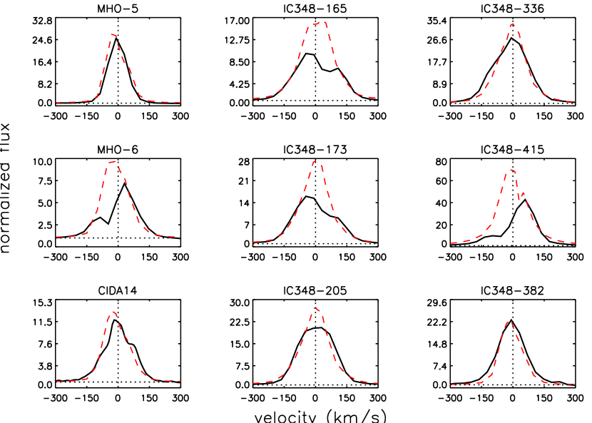
Figure 7: Comparison of observed and model H$\alpha\;$profiles for the 9 accretors with spectral types $>$ M4. Note that the models do not include a wind component, and hence cannot reproduce the blueshifted absorption components seen in MHO-6 and IC348-415. Discrepancies near line center are likely due to rotation effects or a breakdown of the Sobolev approximation (see text).

For each accretor H$\alpha\;$profile, we constructed a model by adopting the above parameter constraints, varying only the mass accretion rate and inclination angle to find the best match to the observed profile shape and flux. A range of accretion rates were explored, $10^{-12}<\dot{M}<10^{-9}\;\rm M_{\odot}\,yr^{-1}$, with the lower limit set where accretion emission is produced at an undetectable level, and the upper limit set by the veiling constraints. The inclination angle was varied from pole-on to edge-on orientations of the star/disk system. Our best model matches are shown in Figure 7, with parameters listed in Table 6. We have not modeled the 3 accretors earlier than M5, due to the temperature parameter degeneracy problem mentioned above (we did derive accretion rates from the veiling for two of these, Haro 6-28 and LkH$\alpha\;$358, with $\dot{M}>10^{-9}\;\rm M_{\odot}\,yr^{-1}$ in both cases; see Figure 5). We also do not show a model for V410 Anon 13, the subject of an earlier paper (Muzerolle et al. 2000b). Note that in two objects shown in Figure 7, MHO-6 and IC348-415, the H$\alpha\;$profiles show blueshifted absorption components. Such features are produced in accretion-powered winds, which are not treated in the model calculations. In these cases, we have tried to match only the red and high-velocity blue wings.

The overall agreement between the observed and model profiles is remarkably good, especially considering the idealized model geometry. In reality, the accretion flows are probably not axisymmetric, and in many cases may be broken up into discrete “streams” (e.g., Muzerolle et al. 2000b). The discrepancies near line center for some of the IC 348 objects (higher predicted flux than observed) may be a result of neglecting rotation in the model calculations; we do not have rotation velocities for those objects, which could conceivably be rotating much faster than typical of the Taurus objects in the HIRES subsample. Previous models we have generated for higher-mass stars with rapid rotation generally produce somewhat broader, less-strongly peaked profiles with doubling at line center. In addition, the assumption of a large velocity gradient implicit in our use of the Sobolev approximation in the model calculations for the line source function break down near line center, which mainly probes the outermost region of the magnetospheric flow where velocities are relatively small and densities are correspondingly large. Thus, we may be overestimating the amount of flux that can escape from the outer regions of the magnetosphere. Nevertheless, these models provide quantitative estimates of mass accretion rates (which we show in Tables 4 and 5) that are accurate to within a factor of $\sim$3-5, given the preceding caveats. Note that these H$\alpha\;$-derived accretion rates are consistent with the values and upper limits derived from the veiling, as shown in the previous section. Although our $\dot{M}$ estimates are not as accurate as UV excess measurements, they are likely the best achievable constraints for VLM objects at present, given the generally small accretion rates, which yield only a small amount of excess emission in the UV.

6 Discussion

The clear signatures of accretion exhibited in roughly 30% of our late-type sample indirectly reveal the presence of circumstellar accretion disks, and indicate that such disks are relatively common in young VLM objects. Observations of infrared excesses yield further evidence of disk accretion, and several recent studies along these lines have shown that the fraction of VLM young stars and brown dwarfs with disks is indeed – and not surprisingly – similar to that of the higher mass TTSs (e.g., Muench et al. 2001; Liu, Najita & Tokunaga 2002). Examination of Table 1 shows that a fairly large fraction of our sample exhibits near-infrared excess, indicative of circumstellar disks. The level of excess at these wavelengths suggests circumstellar disks with fairly small inner holes, relatively consistent with the inner magnetospheric radius of our H$\alpha\;$models. However, most of the excesses are fairly small ($\Delta(H-K)\lesssim 0.2$), and we cannot definitively rule out spots, spectral type mismatches, or cooler, unresolved companions as possible sources of apparent excess.

In any case, the general agreement between the observed and model H$\alpha\;$profiles we present here shows that magnetically mediated accretion from a disk is applicable to VLM young objects. Thus, the disk accretion paradigm, which is a common (if not universal) aspect of early stellar evolution, appears to work over a very large range of masses, from substellar objects with $M<0.08\rm M_{\odot}$ to at least the highest-mass TTS at $M\sim 2\;\rm M_{\odot}$ (and possibly to even higher masses, including the Herbig Ae/Be stars, some of which exhibit magnetospheric infall signatures; Muzerolle et al. in preparation). A key parameter in the physical description of accretion is the mass accretion rate, which guides both the growth of a young star/brown dwarf and the evolution of its disk. Mass accretion rates have been measured extensively at typical TTS masses of $0.5-1.5\;\rm M_{\odot}$ (e.g. Valenti et al. 1993; Hartigan, Edwards, & Ghandour 1995; Gullbring et al. 1998; Hartmann et al. 1998; White & Ghez 2001); however, in most cases the mass ranges probed have not been sufficiently broad or complete to effectively study any mass dependences. Rebull et al. (2000; 2002) did estimate $\dot{M}$ for $M\sim 0.25-1\;\rm M_{\odot}$ stars in Orion and NGC 2264 using $U$-band excesses, and found a loose correlation with $\dot{M}\propto M$. However, their photometrically-selected samples are incomplete at average or lower values of $\dot{M}$, and rather large extinction uncertainties result in a more uncertain $U$-excess calibration.

More recently, WB03 attempted to measure accretion rates from continuum veiling in a sample of VLM objects in Taurus (including four objects in common with our sample). Most of their sample lacked measurable veiling (as does ours), yielding upper limits on accretion rates of the order $10^{-10}\;\rm M_{\odot}\,yr^{-1}$. They did find two objects with $M<0.2\;\rm M_{\odot}$, including one probable brown dwarf, that exhibited considerable veiling, yielding accretion rates of approximately $2-3\times 10^{-9}\;\rm M_{\odot}\,yr^{-1}$. Together with our previously reported accretion rate for VLM object V410 Anonymous 13 (Muzerolle et al. 2000b), and values for higher-mass Taurus TTS, WB03 also find an approximate correlation of $\dot{M}\propto M$. However, the number of $\dot{M}$ values at the lowest masses that are not upper limits is small.

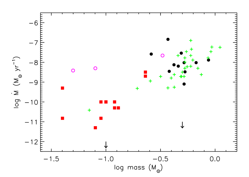
Figure 8: Mass accretion rates as a function of stellar/substellar mass. Squares represent $\dot{M}$ values determined from H$\alpha\;$modeling and veiling in this work and Muzerolle et al. (2000a); solid circles are from Gullbring et al. (1998) (omitting binaries); pluses are from White & Ghez (2000) (including binary components); open circles are from White & Basri (2003). The arrows represent lower limits to $\dot{M}$ at 0.1 and 0.5 $\rm M_{\odot}$ measurable from H$\alpha\;$, as determined from the accretion models.

With H$\alpha\;$modeling, we can probe to accretion rates several orders of magnitude lower than possible from veiling/UV excesses. Figure 8 shows our derived $\dot{M}$ values as a function of mass, along with the WB03 results, and values for higher-mass TTS from Gullbring et al. (1998) and White & Ghez (2001). Note that WB03 and White & Ghez (2001) used the Baraffe et al. (1998) pre-main sequence evolution tracks to determine masses; we have scaled those masses, as well as their values of $\dot{M}$ (since they used $\dot{M}=L_{acc}R_{*}/GM_{*}$), to the D’Antona & Mazzitelli (1998) evolution tracks in order to be consistent with our results. There is a clear correlation between mass accretion rate and stellar/substellar mass, with an approximate proportionality of $\dot{M}\propto M^{2}$. Such a dependence is steeper than in previous investigations.

There are several caveats that must be emphasized when interpreting the above result. One is that the derived (sub)stellar masses are dependent on which evolutionary tracks are used; for example, the Baraffe et al. (1998) tracks yield systematically larger masses, by a factor of $\sim$ 1.5-2. This also affects accretion rates derived from veiling or the UV excess, since those methods require the stellar mass and radius in order to derive $\dot{M}$ from the accretion luminosity. However, we checked the mass-$\dot{M}$ comparison using Baraffe et al. (1998) masses, and find the same proportionality.

Another caveat is that objects accreting at levels low enough that H$\alpha\;$emission from the accretion flow (or UV emission from the accretion shock) is undetectable, would be missed in all surveys conducted to date. Such an effect is probably more relevant to the VLM objects since the minimum $\dot{M}$ at $0.1\;\rm M_{\odot}$ needed to produce observable H$\alpha\;$emission, as determined from our models, is within about a factor of 2 of the lowest measured value in our VLM sample. At $0.5\;\rm M_{\odot}$, the models indicate a higher minimum $\dot{M}$ (since the higher mass of the central object results in higher infall velocities, which in turn results in smaller magnetospheric gas densities for the same accretion rate), but one which is over one order of magnitude lower than the lowest measured value at that mass. Thus, at least at the higher-mass TTSs, the observed lower limit to $\dot{M}$ is probably real.

A final caveat is that VLM objects accreting at rates higher than those measured thus far could be missed due to either veiling completely filling in photospheric features, or very high extinctions. However, the number of so-called “continuum stars” is fairly small (6 in Taurus, as listed in Kenyon & Hartmann 1995), and not necessarily all are VLM objects. One of three Taurus continuum stars observed by WB03, GN Tau, turned out to be M2.5; the other three in Hartmann & Kenyon (1995) have bolometric luminosities higher than likely for accreting VLM objects. Also, there is no evidence for any correlation between extinction and accretion activity in TTSs (not including embedded “Class I” objects). Furthermore, in the extinction-limited sample of Briceño et al. (2002), no correlation between extinction and (sub)stellar mass up to $A_{V}\sim 4$ was seen, thus there is no evidence that young brown dwarfs are selectively more extincted than higher-mass TTSs.

The physical basis for a mass vs. $\dot{M}$ relation is not entirely clear. In the standard model of viscous disk accretion (e.g., Lynden-Bell & Pringle 1974), the disk mass accretion rate is proportional to the disk surface density times the viscosity. The currently favored viscosity mechanism, the Balbus-Hawley instability (e.g., Balbus & Hawley 1998), requires sufficient ionization of the disk gas to operate efficiently. A likely source of ionization of T Tauri disks is X-ray radiation produced by magnetic activity (Glassgold, Najita, & Igea 1997; Igea & Glassgold 1999). Interestingly, recent studies have revealed a fairly strong correlation between X-ray luminosity and mass in young stellar objects (Feigelson et al. 2003; Flaccomio et al. 2003; Mokler & Stelzer 2002; Preibisch & Zinnecker 2002), where $L_{X}$ on average decreases by a factor of $\sim 50-100$ from 1 to 0.1 M_⊙. It is possible that the lower X-ray flux produced by less massive young stars could result in smaller accretion rates by way of decreased disk ionization fractions, driving the correlation we find between $\dot{M}$ and mass. However, it is not clear whether the difference in $L_{X}$ over the mass range represented in Figure 8 can create enough of a change in disk ionization levels to produce a relation as steep as $\dot{M}\propto M^{2}$. On the other hand, the correlation we have determined may be artificially steep, due to the possible selection effects described above. In any case, our results should provide interesting new motivation for continued theoretical work on disk accretion and evolution in young stars and VLM objects.

It should be noted that the mass-$\dot{M}$ relation we find is for objects with a relatively narrow range of ages, $\sim 1-3$ Myr. Thus, we cannot make any conclusions about whether such a relation holds at younger ages, i.e., at the embedded proto(sub)stellar phase. Most of the mass is probably accreted during the first few $\times 10^{5}$ years, either in the initial cloud collapse, or via FU Orionis- type outbursts, which may be different from typical viscous accretion and hence may be unrelated to the scenario we suggest in the previous paragraph. The accretion rates measured here are indicative of a more quiescent, steady accretion phase, and do not have much impact on the subsequent mass evolution of these objects.

We can comment on the fraction of accretors as a function of (sub)stellar age and mass. We have found 13 low-mass accretors with $\dot{M}>10^{-12}\;\rm M_{\odot}\,yr^{-1}$, all of which reside in the young (1-3 Myr) IC 348 or Taurus associations. Conversely, we have found no low mass accretors in the somewhat older (3-8 Myr) Sigma Ori or Sco Cen associations. Consistent with previous results on the evolution of disk accretion in higher mass, $\sim 0.5\;M_{\odot}$, stars (e.g. Muzerolle et al 2000a; Muzerolle et al. 2001b), we find here an accretion timescale on the order of several Myr for objects near the substellar boundary. At mass $\sim 0.5\;M_{\odot}$ and age $\sim 2$ Myr, the fraction of stars identified as accretors is about 50% (e.g., Kenyon & Hartmann 1995 for Taurus). Here, although we have found only about 30% of our total $<0.2\;M_{\odot}$ sample to be accreting, $\sim$50% of the Taurus sample is accreting, albeit at lower rates.

Table 1: (Sub)Stellar Properties of the Observed Sample

object	Spec. Type	log $L_{bol}$ (L⊙)	$I$	$J-H$	$H-K$	$K$	$A_{V}$	$\Delta(H-K)$	log age (yr)	mass (M⊙)
CIDA 13	M3.5	-1.47	13.95	0.61	0.20	11.85	0.35	-0.08	6.94	0.19
CIDA 14	M5	-0.64	12.24	0.67	0.33	9.41	0.34	-0.01	5.10	0.12
FN Tau	M5	-0.30	$\cdots$	0.95	0.50	8.25	1.35	0.10	$<$5.00	0.11
FP Tau	M2.5	-0.49	11.33	0.69	0.25	8.97	0.24	0.00	5.88	0.22
Haro 6-28	M2.5	-0.82	$\cdots$	1.07	0.74	9.27	1.77	0.39	6.23	0.23
LkCa 1	M4	-0.44	11.07	0.77	0.24	8.69	0.00	0.01	5.79	0.21
LkHa 358	K7-M0	0.88	16.05	2.09	1.21	9.69	13.6	0.19	$<$5.00	0.23
MHO-4	M7	-1.14	14.32	$\cdots$	$\cdots$	$\cdots$	0.97	$\cdots$	5.06	0.06
MHO-5	M6	-1.18	13.72	0.63	0.48	10.05	0.11	0.11	5.63	0.09
MHO-6	M4.75	-1.16	13.80	0.71	0.42	10.63	0.86	0.06	6.31	0.13
MHO-7	M5.25	-0.97	13.18	0.65	0.29	10.15	0.40	-0.06	5.62	0.12
MHO-8	M6	-1.02	13.63	0.74	0.38	9.74	0.62	-0.02	5.42	0.09
MHO-9	M5	-0.47	12.95	$\cdots$	$\cdots$	$\cdots$	2.22	$\cdots$	$<$5.00	0.11
V410Anon 13	M5.75	-1.45	16.59	1.24	0.71	10.95	3.83	0.12	6.51	0.08
V410 Xray-3	M6	-1.20	14.18	0.71	0.39	10.39	0.80	-0.02	5.66	0.09
V410 Xray-5a	M5.5	-1.29	15.37	1.24	0.61	10.14	2.57	0.11	6.33	0.10
V927 Tau	M3.5	-0.46	11.46	0.86	0.31	8.68	0.38	0.02	5.17	0.15
IC348-165	M5.25	-0.98	16.07	0.81	0.50	11.77	2.41	0.02	5.64	0.12
IC348-173	M5.75	-0.95	$\cdots$	0.72	0.53	11.85	1.42	0.09	5.40	0.10
IC348-205	M6	-1.11	$\cdots$	0.69	0.65	12.15	1.21	0.21	5.52	0.09
IC348-336	M5.5	-1.40	17.61	0.91	0.63	13.27	3.12	0.10	6.42	0.10
IC348-363	M8	-2.12	17.95	0.64	0.69	13.50	0.00	0.24	5.37	0.02
IC348-382	M6.5	-1.91	18.92	0.87	0.76	13.72	2.77	0.20	5.69	0.04
IC348-407	M7	-2.01	19.71	0.88	1.41	13.97	3.55	0.78	5.37	0.03
IC348-415	M6.25	-2.00	18.23	0.67	0.12	14.03	1.35	-0.34	6.07	0.04
IC348-454	M5.75	-2.19	17.82	0.88	0.31	14.31	0.11	-0.04	6.84	0.05
IC348-478	M6.25	-1.92	18.58	1.13	0.40	14.64	2.27	-0.11	5.98	0.04
SOri-12	M6	-1.51	16.47	0.56	0.36	13.28	0.00	0.00	6.31	0.07
SOri-17	M6	-1.70	16.95	0.58	0.40	13.79	0.00	0.04	6.46	0.06
SOri-25	M6.5	-1.75	17.16	0.51	0.40	13.76	0.00	0.02	5.62	0.04
SOri-29	M6	-1.81	17.23	0.53	0.34	13.96	0.00	-0.02	6.54	0.05
SOri-40	M7	-2.09	18.09	0.54	0.36	14.59	0.00	-0.05	5.39	0.02
SOri-45	M8.5	-2.62	19.59	0.65	0.37	15.66	0.00	-0.09	5.98	0.02
SOri-46	M8.5	-2.71	19.82	0.65	0.37	15.66	0.00	-0.09	6.09	0.02
UScoCTIO-66	M6	-1.55	14.85	0.60	0.38	11.92	0.00	0.02	6.34	0.07
UScoCTIO-75	M6	-1.64	15.08	$\cdots$	$\cdots$	$\cdots$	0.00	$\cdots$	6.41	0.06
UScoCTIO-85	M6	-1.70	15.23	0.58	0.39	11.95	0.00	0.03	6.46	0.06
UScoCTIO-100	M7	-1.78	15.62	0.62	0.40	11.83	0.00	-0.01	5.31	0.03
UScoCTIO-109	M6	-2.03	16.06	$\cdots$	$\cdots$	$\cdots$	0.00	$\cdots$	6.71	0.04
UScoCTIO-121	M6	-2.19	16.46	0.61	$\cdots$	$\cdots$	0.00	$\cdots$	6.79	0.04
UScoCTIO-128	M7	-2.37	17.09	0.63	$\cdots$	$\cdots$	0.00	$\cdots$	5.47	0.02
UScoCTIO-132	M7	-2.59	17.63	0.77	$\cdots$	$\cdots$	0.00	$\cdots$	6.07	0.02
GY 5	M7	-0.96	$\cdots$	1.13	0.66	10.91	5.00	-0.06	$<$5.00	0.07
GY 37	M6	-1.94	$\cdots$	1.31	0.95	11.99	3.30	0.38	6.64	0.05
GY 141	M8.5	-2.59	$\cdots$	0.76	0.50	13.87	0.00	0.04	5.93	0.02

Note. — The photometry and spectroscopy used to calculate extinction values, infrared excesses, effective temperatures and luminosities comes from the following sources: Taurus – 2MASS, Briceno et al. (1999), Briceno et al. (1998), Luhman & Rieke (1998), Kenyon & Hartmann (1995); IC 348 – Luhman (1999), Luhman et al. (1998), Herbig (1998), Najita et al. (2000); Sigma Ori – 2MASS, Bejar et al. (1999) and Bejar et al. (2001); Upper Sco – 2MASS, Ardila, Martín, & Basri (2000) Ophiuchus – Wilking, Greene, & Meyer (1999), Luhman & Rieke (1999), Barsony et al. (1997).

Table 2: Velocities & Lithium

object	Vr	$v\sin i$	EW(Li $\lambda$6708)
CIDA 13	15.9 $\pm$ 0.5	$\cdots$	$<$0.1
CIDA 14	14.0 $\pm$ 0.7	11.8 $\pm$ 1.8	0.51
FN Tau	14.9 $\pm$ 0.4	8.5 $\pm$ 0.8	0.52
FP Tau	16.8 $\pm$ 2.0	34.2a $\pm$ 0.8	0.58
Haro 6-28	16.8 $\pm$ 0.9	$\cdots$	0.6
LkCa 1	9.0 $\pm$ 1.8	34.4a $\pm$ 0.6	0.55
LkHa 358 (ESI)	8.9 $\pm$ 4.6	$\cdots$	0.4
LkHa 358 (HIRES)	17.9 $\pm$ 3.1	20.4 $\pm$ 1.1	0.58
MHO-4	19.1 $\pm$ 0.8	$\cdots$	0.5
MHO-5	12.3 $\pm$ 1.2	$\cdots$	0.5
MHO-6	13.6 $\pm$ 0.7	$\cdots$	0.5
MHO-7	16.9 $\pm$ 0.8	$\cdots$	0.5
MHO-8 (ESI)	15.9 $\pm$ 0.9	$\cdots$	0.5
MHO-8 (HIRES)	15.3 $\pm$ 1.5	16.7 $\pm$ 2.4	0.57
MHO-9	13.8 $\pm$ 0.5	$\cdots$	0.6
V410 Anon 13 (ESI)	20.4 $\pm$ 0.9	$\cdots$	0.5
V410 Anon 13 (HIRES)	15.1 $\pm$ 1.3	9.8 $\pm$ 3.0	0.65:
V410 Xray 3	14.6 $\pm$ 0.9	$\cdots$	0.5
V410 Xray 5	14.7 $\pm$ 0.4	$\cdots$	0.6
V927 Tau	16.5 $\pm$ 0.6	13.3 $\pm$ 1.3	0.33
IC348-165	8.8 $\pm$ 0.6	$\cdots$	0.5
IC348-173	13.9 $\pm$ 2.4	$\cdots$	0.5
IC348-205	15.7 $\pm$ 3.4	$\cdots$	0.8
IC348-336	13.5 $\pm$ 3.0	$\cdots$	$\cdots$
IC348-363	9.5 $\pm$ 1.7	$\cdots$	$\cdots$
IC348-382	9.1 $\pm$ 0.6	$\cdots$	$\cdots$
IC348-407	7.9 $\pm$ 2.6	$\cdots$	$\cdots$
IC348-415	14.7 $\pm$ 2.5	$\cdots$	1.1:
IC348-454	10.5 $\pm$ 1.8	$\cdots$	0.6
IC348-478	10.8 $\pm$ 1.4	$\cdots$	$\cdots$
SOri-12	29.8 $\pm$ 0.7	$\cdots$	0.6
SOri-17	19.66 $\pm$ 1.7	$\cdots$	0.8:
SOri-25 (ESI)	30.06 $\pm$ 2.5	$\cdots$	0.6
SOri-25 (HIRES)	29.6 $\pm$ 2.3	9.4 $\pm$ 1.0	$\cdots$
SOri-29	27.1 $\pm$ 1.6	$\cdots$	0.6
SOri-40	32.5 $\pm$ 3.3	$\cdots$	0.5
SOri-45	22.4 $\pm$ 5.3	$\cdots$	$\cdots$
SOri-46	55.8 $\pm$ 2.9	$\cdots$	$\cdots$
UScoCTIO 66	-4.4 $\pm$ 0.6	$\cdots$	0.6
UScoCTIO 75	-5.6 $\pm$ 1.1	$\cdots$	0.6
UScoCTIO 85	-24.6 $\pm$ 0.7	$\cdots$	$<$0.1
UScoCTIO 100	-8.9 $\pm$ 0.6	$\cdots$	0.6
UScoCTIO 109	-3.8 $\pm$ 0.7	$\cdots$	0.6
UScoCTIO 121	-38.9 $\pm$ 1.0	$\cdots$	$<$0.3
UScoCTIO 128	-3.0 $\pm$ 1.6	$\cdots$	0.5:
UScoCTIO 132	-8.2 $\pm$ 1.1	$\cdots$	$<$0.4:
GY 5	-6.3 $\pm$ 1.9	16.8 $\pm$ 2.7	0.5
GY 37	$\cdots$	$\cdots$	$\cdots$
GY 141	$\cdots$	$\cdots$	$\cdots$

Note. — Velocities in km s^-1, EW in Å. Null values indicate that measurements could not be made due to low continuum S/N, or, in the case of $v\sin i$, could not be made due to the lower resolution of the ESI spectrograph.

^aPossible spectroscopic binary.

Table 3: Emission Lines

object	H$\alpha\;$	H$\alpha\;$	H$\beta$	H$\gamma$	H$\delta$	He I	[OI]	[OI]	Ca II	Ca II	Ca II	accretor?	instrument
	10% width					$\lambda$5876	$\lambda$6300	$\lambda$6363	$\lambda$8498a	$\lambda$8542a	$\lambda$8662a
CIDA 13c	77	-1.6	-2.0	-2.0	-2.0	-0.4	$<$-0.1	$<$-0.1	$<$-0.1	$<$-0.6	$<$-0.6	n	ESI
CIDA 14	289	-34	$\cdots$	$\cdots$	$\cdots$	$\cdots$	$\cdots$	$<$-0.1	$<$-0.2	$\cdots$	$<$-0.1	y	HIRES
FN Tau	195	-22	$\cdots$	$\cdots$	$\cdots$	$\cdots$	$\cdots$	$<$-0.2	-0.9	$\cdots$	-0.7	n	HIRES
FP Tau	418	-32	$\cdots$	$\cdots$	$\cdots$	$\cdots$	$\cdots$	$<$-0.1	-0.1	$\cdots$	-0.1	y	HIRES
Haro 6-28	347	-48	-30	-25	-25	-2.2	-1.2	-0.3	-0.2	-0.3	-0.1	y	ESI
LkCa 1	178	-3.9	$\cdots$	$\cdots$	$\cdots$	$\cdots$	$\cdots$	$<$-0.1	-0.1	$\cdots$	$<$-0.1	n	HIRES
LkH$\alpha\;$358	502	-63	-22b	$\cdots$	$\cdots$	-1.9	-15	-4.1	-6.3	-6.6	-5.1	y	ESI
LkH$\alpha\;$358	477	-62	$\cdots$	$\cdots$	$\cdots$	$\cdots$	$\cdots$	-2.2	-9.1	$\cdots$	-7.8	y	HIRES
MHO-4	116	-43	-56	-35	-25	-4.3	1.2:	$<$-0.1	-0.4	-0.5	-0.1	n	ESI
MHO-5	154	-60	-44	-29	-19	-3.3	-4.0	-0.9	-0.4	-0.5	-0.1	y	ESI
MHO-6	309	-25	-13	-11	-8.6	-1.7	-1.4	-0.3	$<$-0.1	$<$-0.1	$<$-0.1	y	ESI
MHO-7	116	-9.0	-7.5	-3.6	-3.0	-0.5	$<$-0.1	$<$-0.1	$<$-0.1	$<$-0.1	$<$-0.1	n	ESI
MHO-8	115	-18	-17	-11	-5.5	-1.4	$<$-0.1	$<$-0.1	$<$-0.2	$<$-0.1	$<$-0.1	n	ESI
MHO-8	128	-14	$\cdots$	$\cdots$	$\cdots$	$\cdots$	$\cdots$	$<$-0.1	$<$-0.2	$\cdots$	$<$-0.2	n	HIRES
MHO-9	116	-3.5	-4.3	-2.8	-2.4	-0.5	$<$-0.2	$<$-0.1	$<$-0.1	$<$-0.3	$<$-0.2	n	ESI
V410 Anon 13	270	-29	-20b	-9b	$\cdots$	-12.8b	-0.8	$<$-0.5	$<$-0.1	$<$-0.1	$<$-0.1	y	ESI
V410 Anon 13	248	-27	$\cdots$	$\cdots$	$\cdots$	$\cdots$	$\cdots$	$<$-0.4	$<$-0.3	$\cdots$	$<$-0.1	y	HIRES
V410 Xray-3	116	-20	-23	-18	-10	-2.4	$<$-0.2	$<$-0.1	$<$-0.1	$<$-0.2	$<$-0.1	n	ESI
V410 Xray-5a	154	-19	-22	-15b	$\cdots$	-2.1	$<$-0.5	$<$-0.2	-0.2	-0.3	$<$-0.1	n	ESI
V927 Tau	290	-7.0	$\cdots$	$\cdots$	$\cdots$	$\cdots$	$\cdots$	$<$-0.1	$<$-0.1	$\cdots$	$<$-0.1	n	HIRES
IC348-165	347	-54	-28	-24b	$\cdots$	-2.4	-0.3:	-0.2	-0.3:	-0.4	-0.4:	y	ESI
IC348-173	347	-86	-50	-10b	-35b	-7.5	-2.2:	-0.4	-0.8	-1.6	-0.7	y	ESI
IC348-205	270	-105	-74b	$\cdots$	$\cdots$	$<$-1.5b	$<$-0.5	$<$-0.7	-1.1	-1.8	-0.9	y	ESI
IC348-336	309	-121	-42b	-20b	$\cdots$	-6.4b	$<$-2.8:	$<$-1.1:	-0.2	-0.4	$<$-0.1	y	ESI
IC348-363	117	-13	$\cdots$	$\cdots$	$\cdots$	$\cdots$	$<$-21:	$<$-1.0	$<$-0.1	$<$-0.1	$<$-0.1	n	ESI
IC348-382	232	-70	$\cdots$	$\cdots$	$\cdots$	$\cdots$	$\cdots$	$\cdots$	-0.6	-0.9	-0.3:	y	ESI
IC348-407	155	-24	$\cdots$	$\cdots$	$\cdots$	$\cdots$	$\cdots$	$\cdots$	$<$-0.7	-0.7:	$<$-1.1	n	ESI
IC348-415	272	-152	-40b	$\cdots$	$\cdots$	$\cdots$	$<$-4.0:b	$<$-1.3	-2.8	-4.7	-2.6	y	ESI
IC348-454	193	-23	-32b	-18b	$\cdots$	$\cdots$	$<$-3.5:	$<$-3.9	$<$-0.1	$<$-0.1	$<$-0.2	n	ESI
IC348-478	117	-22	-40b	$\cdots$	$\cdots$	$\cdots$	$<$-9.6:	$<$-1.5	$<$-0.1	$<$-0.2	$<$-0.1	n	ESI
SOri-12	116	-9	-9.5	-5.5b	$\cdots$	$\cdots$	$<$-1.1:	$<$-0.3	$<$-0.1	$<$-0.1	$<$-0.1	n	ESI
SOri-17	126	-4.8	-5.0b	$\cdots$	$\cdots$	$\cdots$	$<$-3.5:	$<$-2.2:	$<$-0.1	$<$-0.1	$<$-0.1	n	ESI
SOri-25	156	-44	-50b	-36b	$\cdots$	-6.0	$<$-1.0	$<$-0.5	-0.2:	-0.2	$<$-0.2	n	ESI
SOri-25	94:	-36b	$\cdots$	$\cdots$	$\cdots$	$\cdots$	$\cdots$	$\cdots$	$<$-0.5	$\cdots$	$<$-0.25	n	HIRES
SOri-29	154	-15	-21	-16b	$\cdots$	$<$-1.5	$<$-0.2	$<$-0.1	$<$-0.1	$<$-0.1	$<$-0.2	n	ESI
SOri-40	194	-16	-12	$\cdots$	$\cdots$	$\cdots$	$<$-1.0:	$<$-2.3:	$<$-0.1	$<$-0.3	$<$-0.2	n	ESI
SOri-45c	78:	-21b	-16b	$\cdots$	$\cdots$	$\cdots$	$\cdots$	$\cdots$	$<$-0.2	$<$-0.3	$<$-1.4	n	ESI
SOri-46c	194	-14	-9b	$\cdots$	$\cdots$	$\cdots$	$\cdots$	$\cdots$	$<$-0.4	$<$-0.4	$<$-0.6	n	ESI
UScoCTIO-66	116	-6.0	-8.8	-8.0	-5.5	-1.0	$<$-0.3	$<$-0.1	$<$-0.1	$<$-0.1	$<$-0.1	n	ESI
UScoCTIO-75	231	-15	-19	-16	-10	-1.3	$<$-0.1	$<$-0.1	$<$-0.1	$<$-0.1	$<$-0.1	n	ESI
UScoCTIO-85c	154	-7.0	-14	-18b	-5.0b	-0.9	$<$-0.2	$<$-0.2	$<$-0.1	$<$-0.2	$<$-0.2	n	ESI
UScoCTIO-100	154	-12	-23	-20	-12	-2.0	$<$-0.1	$<$-0.1	$<$-0.1	$<$-0.1	$<$-0.1	n	ESI
UScoCTIO-109	116	-10	-22	-12	-11b	-2.5	$<$-0.3	$<$-0.1	$<$-0.2	$<$-0.1	$<$-0.1	n	ESI
UScoCTIO-121c	116	-7.3	-25b	$\cdots$	$\cdots$	$\cdots$	$<$-0.4:	$<$-1.2	$<$-0.1	$<$-0.1	$<$-0.2	n	ESI
UScoCTIO-128	193	-60	-50	-50b	-30b	-10b	$<$-0.3	$<$-0.6	-0.3	-0.6	$<$-0.2	n	ESI
UScoCTIO-132c	116	-4	$\cdots$	$\cdots$	$\cdots$	$\cdots$	$<$-3.0:	$<$-0.6	$<$-0.2	$<$-0.3	$<$-0.4	n	ESI
GY 5	177	-17	$\cdots$	$\cdots$	$\cdots$	$\cdots$	$\cdots$	-0.4:	$<$-0.2	$\cdots$	$<$-0.1	n	HIRES
GY 37	197:	-20b	$\cdots$	$\cdots$	$\cdots$	$\cdots$	$\cdots$	$\cdots$	$<$-0.4	$\cdots$	$<$-0.4	n	HIRES
GY 141	88:	-32b	$\cdots$	$\cdots$	$\cdots$	$\cdots$	$\cdots$	$\cdots$	$<$-3.0	$\cdots$	$<$-17	n	HIRES
Gl 406	113	-7.1	-13	-15	-16	-0.9d	$<$-0.1	$<$-0.1	$<$-0.1	-0.1	$<$-0.1	n	ESI
LHS 2351	136	-3.9	-11	-9.2	-9.1b	-0.6d	$<$-0.1	$<$-0.1	$<$-0.1	-0.2:	$<$-0.2	n	ESI

Note. — Line measurements are equivalent widths in Å, unless otherwise noted. H$\alpha$ 10% widths are in km s^-1. Colons indicate uncertain measurements due to poor S/N, or imperfect sky subtraction at the [OI] lines. Accretors have been selected based on H$\alpha\;$characteristics, as described in section 4. Gl406 and LHS 2351, main sequence dwarfs with spectral types M5.5 and M7Ve, respectively, are included for comparison.

^a Ca II EW of emission component; measured against absorption pseudo-continuum when photospheric absorption component is not completely filled in by the emission.

^b Continuum not detected at line position.

^c Most likely not a member of the association (see text).

^d Measured from a pseudo-continuum within absorption wing of Na I line.

Table 4: ESI Accretor Sample

object	veiling template	r5500	r6200	r7100	r8900	log $\dot{M}\;(\rm M_{\odot}\,yr^{-1})$
Haro 6-28	TWA 15A, CIDA 13a	0.3	0.2	0.1	0.0	-8.7b
LkH$\alpha\;$358	LkCa 7	$\cdots$	1.0:	1.0:	1.0:	-8.5b
MHO-5	V410 Xray-3	0.0	0.1	0.0	0.0	-10.8
MHO-6	MHO-7	0.0	0.1	0.1	0.1	-10.3
V410 Anon13	V410 Xray-3	0.0	0.1	0.0	0.1	-11.3
IC348-165	MHO-8	0.0	0.0	0.0	0.0	-10
IC348-173	MHO-7	0.0	0.1	0.0	0.0	-10
IC348-205	MHO-8	0.0:	0.1	0.0	0.1	-10
IC348-336	MHO-7	$\cdots$	0.2:	0.1	0.1	-10
IC348-382	V410 Xray-3	$\cdots$	$\cdots$	0.2:	0.2:	-10.8
IC348-415	V410 Xray-3	$\cdots$	0.5:	0.1	0.1	-9.3

Note. — Typical veiling errors are $\sim\pm 0.1$. Colons indicate larger uncertainties due to poor S/N. Null values are cases where the S/N was so low that no measurements could be made. Accretion rates are in $\rm M_{\odot}\,yr^{-1}$, all determined from H$\alpha\;$modeling except for ^b, which were determined from the veiling.

^a Veiling template was the average of these two stars, whose spectral types are M1.5 and M3.5, respectively.

Table 5: Veiling - HIRES Accretor Sample

object	template	r6450	r7100	r8700	log $\dot{M}\;(\rm M_{\odot}\,yr^{-1})$
CIDA 14	MHO-8	-0.1	0.1	-0.1	-10.3
FP Tau	LkCa 1	0.0	0.2	-0.1	$<$-9a
LkH$\alpha\;$358	LkCa 7	0.4	0.4	0.4	-8.5a
V410 Anon 13	MHO-8	$\cdots$	0.1	0.0	-11.3

Note. — Typical veiling errors are $\sim\pm 0.1$. Null value indicates no S/N in the object spectrum around that wavelength. Accretion rates are in $\rm M_{\odot}\,yr^{-1}$, all determined from H$\alpha\;$modeling except for ^a, which were determined from the veiling.

Table 6: Parameters for H$\alpha\;$Model Comparisons

object	$M_{*}\;(M_{\odot})$	$R_{*}\;(R_{\odot})$	$R_{mag}\;(R_{*})$	$T_{max}\;(K)$	$i\;(^{\circ})$	log $\dot{M}\;(\rm M_{\odot}\,yr^{-1})$
MHO-5	0.05	0.5	2.2-3	12,000	45	-10.8
MHO-6	0.15	1.0	2.2-3	12,000	60	-10.3
CIDA 14	0.15	1.0	2.2-3	12,000	50	-10.3
IC348-165	0.15	1.0	2.2-3	12,000	89	-10.0
IC348-173	0.15	1.0	2.2-3	12,000	80	-10.0
IC348-205	0.15	1.0	2.2-3	12,000	80	-10.0
IC348-336	0.15	1.0	2.2-3	12,000	75	-10.0
IC348-415	0.05	0.5	2.2-3	12,000	45	-9.3
IC348-382	0.05	0.5	2.2-3	12,000	55	-10.8

Note. — $R_{mag}$ is the inner and outer radius of the magnetospheric accretion flow at the disk surface. $T_{max}$ is the maximum value of the temperature distribution of the flow. The inclination angle is measured from the axis of rotation of the system.

Figure 1: HR diagram of entire sample, using pre-main sequence tracks of D’Antona & Mazzitelli (1998). Solid triangles represent accretors, open triangles represent non-accretors (see text).

Figure 2: Continuum-normalized H$\alpha\;$profiles; see Table 3 for further information.

Figure 2: Continued.

Figure 2: Continued.

Figure 3: Top panel: distribution of H$\alpha\;$10% line widths for the entire sample (open histogram), and for the accretor subsample (solid histogram). Bottom panel: comparison of H$\alpha\;$10% width versus equivalent width, for accretors (solid circles) and non-accretors (open circles). In both plots, objects where the continuum at H$\alpha\;$was not detected were not included.

Figure 4: Logarithm of the veiling as a function of wavelength for an M5 star (upper panel) and an M6 star (lower panel), representative of our sample. Veiling values are shown for three values of the mass accretion rate, log $\dot{M}$ = -10, -9, and -8, labeled accordingly. Shock models are calculated for an energy flux log ${\cal F}$ = 10 (dotted lines), 11 (solid lines), and 12 (dashed lines). Photospheric colors are taken from Leggett (1992) and Luhman (1999). The horizontal dashed lines represent the minimum measurable veiling level.

Figure 5: Veiling measurements from accretors in Tables 4 and 5 (open circles with error bars), compared to shock models, cf. Figure 4 (solid squares, connected). The value of ${\cal F}$ indicated on each panel matches the spectral shape of the veiling, while $f$ is adjusted to match its level, resulting in the indicated values of $\dot{M}$ in each case (with corresponding errors in log $\dot{M}$ of roughly $\pm$ 0.2-0.3). The estimated filling factors $f$ are 0.06 for LkH$\alpha\;$358, 0.002 for Haro 6-28, 0.01 for IC348-336, and 0.0004 for IC348-415.

Figure 6: Model H$\alpha\;$profiles, as a function of magnetospheric density and temperature. All models calculated with $M_{*}=0.05\,\rm M_{\odot}$, $R_{*}=0.5\,R_{\odot}$, $i=60^{\circ}$, and $R_{mag}=2.2-3\;R_{*}$. Solid line: $\dot{M}=10^{-9}\,\rm M_{\odot}\,yr^{-1}$, $T_{max}=8000\;K$. Dashed line: $\dot{M}=10^{-9}\,\rm M_{\odot}\,yr^{-1}$, $T_{max}=10,000\;K$. Dot-dashed line: $\dot{M}=10^{-10}\,\rm M_{\odot}\,yr^{-1}$, $T_{max}=10,000\;K$. Dotted line: $\dot{M}=10^{-10}\,\rm M_{\odot}\,yr^{-1}$, $T_{max}=12,000\;K$.

References

- (1) Adams, F. C., Lada C. J., & Shu, F. H. 1987, ApJ, 312, 788
- (2) Abdul-Aziz, H., Abranin, E. P., Alekseev, I. Y. et al. 1995, A&AS, 114, 509
- (3) Abranin, E. P., Alekseev, I. Y., Avgoloupis, S. et al. 1998, A&AT, 17, 221
- (4) Alencar, S. H. P. & Batalha, C. 2002, ApJ, 571, 378
- (5) Ardila, D. R., Martín, E., & Basri, G. 2000, AJ, 120, 479
- (6) Balbus, S. A. & Hawley, J. F. 1998, Rev. Mod. Phys., 70, 1
- (7) Baraffe, I., Chabrier, G., Allard, F., & Hauschildt, P. H. 1998, A&A, 337, 403
- (8) Barsony, M, Kenyon, S. J., Lada, E. A., & Teuben, P. J. 1997, ApJS, 112, 109
- (9) Basri, G. & Bertout, C. 1989, ApJ, 341, 340
- (10) Bejar, V. J. S., Zapatero-Osorio, M. R., & Rebolo, R. 1999, ApJ, 521, 671
- (11) Bejar, V. J. S., et al. 2001, ApJ, 556, 830
- (12) Bertout, C., Basri, G., & Bouvier, J. 1988, ApJ, 330, 350
- (13) Bessell, M. S. & Brett, J. M. 1988, PASP, 100, 1134
- (14) Briceño, C., Calvet, N., Kenyon, S., & Hartmann, L. 1999, AJ, 118, 1354
- (15) Briceño, C., Hartmann, L., Stauffer, J., & Martín, E. 1998, AJ, 115, 2074
- (16) Briceño, C., Luhman, K. L., Hartmann, L., Stauffer, J. R., & Kirkpatrick, J. D. 2002, ApJ, 580, 317
- (17) Calvet, N. 1997, in IAU Symp. 182, Herbig-Haro Flows and the Birth of Low Mass Stars, ed. B. Reipurth & C. Bertout (Boston: Kluwer), 417
- (18) Calvet, N. & Gullbring, E. 1998, ApJ, 509, 802 (CG98)
- (19) Cohen, M. & Kuhi, L. 1979, ApJS, 41, 743
- (20) Chabrier, G., Baraffe, I., Allard, F., & Hauschildt, P. 2000, ApJ, 542, 464
- (21) D’Antona, F. & Mazzitelli, I. 1997, Mem. Soc. Astron. Italiana, 68, 807
- (22) Delfosse, X., Forveille, T., Perrier, C., & Mayor, M. 1998, A&A, 331, 581
- (23) Edwards, S. et al. 1993, AJ, 106, 372
- (24) Feigelson, E. D., Gaffney, J. A., Garmire, G., Hillenbrand, L. A., & Townsley, L. 2003, ApJ, in press
- (25) Flaccomio, E., Damiani, F., Micela, G., Sciortino, S., Harnden, F. R., Murray, S. S., & Wolk, S. J. 2003, ApJ, 582, 398
- (26) Ghosh, P. & Lamb, F. K. 1979, ApJ, 234, 296
- (27) Glassgold, A. E., Najita, J., & Igea, J. 1997, ApJ, 480, 344
- (28) Gullbring, E., Calvet, N., Muzerolle, J., & Hartmann, L. 2000, ApJ, 544, 927
- (29) Hartigan, P., Edwards, S., & Ghandour, L. 1995, ApJ, 452, 736
- (30) Hartigan, P., Hartmann, L., Kenyon, S., Hewett, R., & Stauffer, J. 1989, ApJS, 70, 899
- (31) Hartmann, L., Calvet, N., Gullbring, E., & D’Alessio, P. 1998, ApJ, 495, 385
- (32) Hartmann, L., Hewett, R., & Calvet, N. 1994, ApJ, 426, 669
- (33) Hartmann, L., Hewett, R., Stahler, S., & Mathieu, R. D. 1986, ApJ, 309, 275
- (34) Herbig, G. H. 1998, ApJ, 497, 736
- (35) Hillenbrand, L. A. & Carpenter, J. M. 2000, ApJ, 540, 236
- (36) Hirose, S., Uchida, Y., Shibata, K., & Matsumoto, R. 1997, PASJ, 49, 193
- (37) Igea, J. & Glassgold, A. E. 1999, ApJ, 518, 848
- (38) Johns-Krull, C. M. & Valenti, J. A. 2000, in ASP Conf. Ser. 198, Euroconference on Stellar Clusters and Associations: Convection, Rotation, and Dynamos, ed. R. Pallavincini, G. Micela, & S. Sciortino (San Francisco: ASP), 371
- (39) Johns-Krull, C. M., Valenti, J. A., Hatzes, A. P., & Kanaan, A. 1999, ApJ, 510, L41
- (40) Kenyon, S. J., Brown, D. I., Tout, C. A., & Berlind, P. 1998, AJ, 115, 2491
- (41) Kenyon, S. J. & Hartmann, L. 1995, ApJS, 101, 117
- (42) Königl, A. 1991, 1991, ApJ, 370, L39
- (43) Leggett, S. K. 1992, ApJS, 82, 351
- (44) Liu, M. C., Najita, J., & Tokunaga, A. T. 2002, ApJ, in press
- (45) Luhman, K. L. 1999, ApJ, 525, 466
- (46) Luhman, K. L. & Rieke, G. H. 1998, ApJ, 497, 354
- (47) Luhman, K. L. & Rieke, G. H. 1999, ApJ, 525, 440
- (48) Luhman, K. L., Rieke, G. H., Lada, C. J., & Lada, E. A. 1998, ApJ, 508, 347
- (49) Lynden-Bell, D. & Pringle, J. E. 1974, MNRAS, 168, 603
- (50) Mannings, V., Boss, A. P., & Russell, S. S. 2000, in Protostars and Planets IV, ed. V. Mannings, A. P. Boss, & S. S. Russell (Tucson: University of Arizona Press)
- (51) Martín, E. L. 1999, MNRAS, 302, 59
- (52) Meyer, M. R., Calvet, N., & Hillenbrand, L. A. 1997, AJ, 114, 288
- (53) Mokler, F. & Stelzer, B. 2002, A&A, 391, 1025
- (54) Muench, A. A., Alves, J., Lada, C. J., & Lada, E. A. 2001, ApJ, 558, L51
- (55) Muzerolle, J., Briceño, C., Calvet, N., Hartmann, L., Hillenbrand, L. A., & Gullbring, E. 2000b, ApJ, 545, L141
- (56) Muzerolle, J., Calvet, N., Briceño, C., Hartmann, L., & Hillenbrand, L. A. 2000a, ApJ, 535, L47
- (57) Muzerolle, J., Calvet, N., & Hartmann, L. 1998a, ApJ, 492, 743
- (58) Muzerolle, J., Calvet, N., & Hartmann, L. 2001a, ApJ, 550, 944 (MCH)
- (59) Muzerolle, J., Hartmann, L., & Calvet, N. 1998b, AJ, 116, 455
- (60) Muzerolle, J., Hillenbrand, L., Calvet, N., Hartmann, L., & Briceño, C. 2001b, in Young Stars Near Earth: Progress and Prospects, ASP Conference Series, Vol. 244, R. Jayawardhana & T. P. Greene, eds.
- (61) Najita, J., Tiede, G. P., & Carr, J. S. 2000, ApJ, 541, 977
- (62) Nidever, D. L., Marcy, G. W., Butler, R. P., Fischer, D. A., & Vogt, S. S. 2002, ApJS, 141, 503
- (63) Preibisch, T. & Zinnecker, H. 2002, AJ, 123, 1613
- (64) Sheinis, A.I., Bolte, M., Epps, H.W., Kibrick, R.I., Miller, J.S., Radovan, M.V., Bigelow, B.C., & Sutin, B.M. 2002, PASP 114, 851
- (65) Shu, F., Najita, J., Ostriker, E., Wilkin, F., Ruden, S., & Lizano, S. 1994, ApJ, 429, 781
- (66) Uchida & Shibata 1985, PASJ, 37, 515
- (67) Vogt, S.S., Allen, S.L., Bigelow, B.C., Bresee, L, et al. 1994, Proc. SPIE 2198, 362
- (68) White, R. J. & Basri, G. 2003, ApJ, 582, 1109 (WB03)
- (69) White, R. J. & Ghez, A. M. 2001, ApJ, 556, 265
- (70) Wilking, B. A., Greene, T. P., & Meyer, M. R. 1999, AJ, 117, 469
- (71) Worden, S. P., Schneeberger, T. J., & Giampapa, M. S. 1981, ApJS, 46, 159
- (72)