The evolution of faint AGN between z $\simeq$ 1 and z $\simeq$ 5 from the COMBO-17 survey

We present a determination of the optical/UV AGN luminosity function and its evolution, based on a large sample of faint ($R<24$) QSOs identified in the COMBO-17 survey. Using multi-band photometry in 17 filters within $350\,\mathrm{nm}\la\lambda_{\mathrm{obs}}\la 930\,\mathrm{nm}$, we could simultaneously determine photometric redshifts with an accuracy of $\sigma_{z}<0.03$ and obtain spectral energy distributions. The redshift range covered by the sample is $1.2<z<4.8$, which implies that even at $z\simeq 3$, the sample reaches below luminosities corresponding to $M_{B}=-23$, conventionally employed to distinguish between Seyfert galaxies and quasars. We clearly detect a broad plateau-like maximum of quasar activity around $z\simeq 2$ and map out the smooth turnover between $z\simeq 1$ and $z\simeq 4$. The shape of the LF is characterised by some mild curvature, but no sharp ‘break’ is present within the range of luminosities covered. Using only the COMBO-17 data, the evolving LF can be adequately described by either a pure density evolution (PDE) or a pure luminosity evolution (PLE) model. However, the absence of a strong $L^{*}$-like feature in the shape of the LF inhibits a robust distinction between these modes. We present a robust estimate for the integrated UV luminosity generation by AGN as a function of redshift. We find that the LF continues to rise even at the lowest luminosities probed by our survey, but that the slope is sufficiently shallow that the contribution of low-luminosity AGN to the UV luminosity density is negligible. Although our sample reaches much fainter flux levels than previous data sets, our results on space densities and LF slopes are completely consistent with extrapolations from recent major surveys such as SDSS and 2QZ.

1 Introduction

The luminosity function of quasi-stellar objects (QSOs) and its evolution with redshift provides one of the most important tools for the cosmic demography of active galactic nuclei (AGN). It constrains physical models for QSOs, particularly those for the growth of supermassive black holes in galaxies within the context of hierachical collapse of structure in the universe (Haehnelt & Rees, 1993; Haiman & Loeb, 1998; Kauffmann & Haehnelt, 2000). It is also relevant for understanding the extragalactic UV background (Meiksin & Madau, 1993; Boyle & Terlevich, 1998).

Previous studies of the QSO luminosity function (QLF) have established a strong rise in the activity with look back time from the local universe to redshifts $z\sim 2$ (Boyle et al., 1988). The main debate at these low to intermediate redshifts is now about the question whether the shape of the QLF changes with redshift (Boyle et al., 2000; Wisotzki, 2000; Miyaji et al., 2000; Cowie et al., 2003). If so, this would mean that low-luminosity AGN evolve differently from high-luminosity QSOs, possibly calling for a substantial revision of our understanding of the cosmic duty cycle of nuclear activity in galaxies.

At higher redshift $z>2$, the obvious expectation that the rise of the QSO activity with redshift must turn over at some point was satisfied by observations at $z>3$ (Warren et al., 1994; Schmidt et al., 1995, hereafter WHO and SSG). However, optical surveys in this redshift regime were often plagued by selection effects and small number statistics. Moreover, studies of X-ray-selected (Miyaji et al., 2000) and radio-selected QSOs (Jarvis & Rawlings, 2000) did not strongly support claims of a very steep drop in nuclear activity for $z>3$, keeping the issue unresolved whether the detected turnover was physical reality or not. A rather robust observation of the space density decline beyond $z>3.6$ has been established recently, albeit only for very luminous QSOs, by the Sloan Digital Sky Survey (SDSS, Fan et al., 2001).

Most optically selected QSO samples are expected to be more or less complete at either $z\la 2.2$ or $z\ga 3.6$, where QSOs show conspicuous colours in broad-band searches, while within this redshift band, confusion arises with stars and compact low-redshift galaxies. Any practical approach of following up QSO samples in this intermediate redshift range is forced to avoid strong contamination and observed mostly extreme objects, resulting in a high degree of incompleteness that is difficult to account for. Thus, while the fact that cosmic QSO activity shows a maximum around $z\simeq 2$–3 is not doubted as such, this maximum has very rarely been detected in a single survey.

This selection issue was one of the original motivations for the COMBO-17 survey. This survey is based on photometric classification and redshift estimation using a set of 17 filters, of which 12 are medium-band filters with $\sim 10,000$ km/sec FWHM, well matched to optimum detection of QSO emission lines and spread across the range of wavelengths observable by modern CCD detectors.

Another major driver for this project was to probe fainter regimes of the AGN luminosity function, a task which has always beed limited by the overwhelming need for spectroscopic follow-up telescope time. Using medium-band spectrophotometry, a reasonably complete and clean AGN sample could be obtained across a wide range of redshifts down to $R\la 24$. Based on such a deep sample, we were able to derive luminosity functions down to $M_{B}\la-23$ at redshifts above 3, entering the domain of Seyfert galaxies even at high redshift.

In this paper, we present a new determination of the luminosity function of faint optically selected QSOs, aimed at a broad redshift range around the elusive turnover. The analysis is based on a sample of 192 objects between $z=1.2$ and $z=4.8$, all selected from the COMBO-17 survey. The survey is briefly described in Sect. 2, followed by a discussion of technical aspects such as completeness and redshift quality in Sect. 3. In Sections 4 through 7 we present and discuss the results.

2 COMBO-17 observations

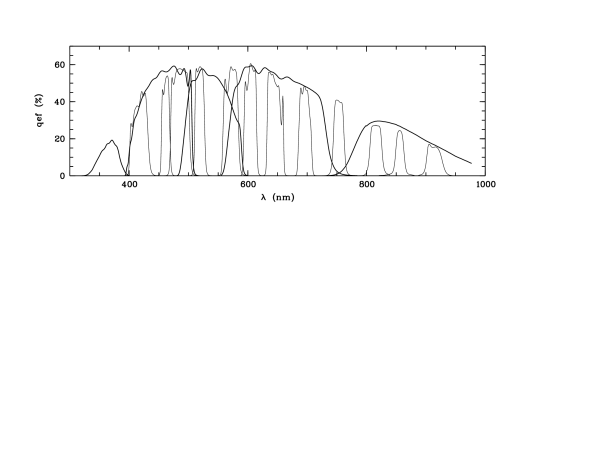
Figure 1: COMBO-17 filter set: Total system efficiencies are shown in the COMBO-17 passbands, including two telescope mirrors, camera, CCD detector and average La Silla atmosphere. Combining all observations provides a low-resolution spectrum for all objects in the field.

Table 1: The COMBO-17 filter set: Exposure times and 10$\sigma$ magnitude limits reached for point sources, averaged over all three fields. The $R$-band observations were selected to be taken under the best seeing conditions (FWHM $0\aas@@fstack{\prime\prime}55\ldots 0\aas@@fstack{\prime\prime}8$). See also Fig. 1.

$\lambda_{\mathrm{\mathrm{cen}}}$/fwhm (nm)		$t_{\mathrm{\mathrm{exp}}}$/sec	$m_{\mathrm{\mathrm{lim},10\sigma}}$
364/38	$U$	20000	23.7
456/99	$B$	14000	25.5
540/89	$V$	6000	24.4
652/162	$R$	20000	25.2
850/150	$I$	7500	23.0
420/30		8000	24.0
462/14		10000	24.0
485/31		5000	23.8
518/16		6000	23.6
571/25		4000	23.4
604/21		5000	23.4
646/27		4500	22.7
696/20		6000	22.8
753/18		8000	22.5
815/20		20000	22.8
856/14		15000	21.8
914/27		15000	22.0

Table 2: Positions and galactic reddening (Schlegel et al., 1998) for the three COMBO-17 fields analysed. All observations were obtained at the Wide Field Imager at the MPG/ESO 2.2 m-telescope at La Silla.

Field	$\alpha_{\mathrm{\mathrm{J2000}}}$	$\delta_{\mathrm{\mathrm{J2000}}}$	$l_{\mathrm{\mathrm{gal}}}$	$b_{\mathrm{\mathrm{gal}}}$	$E_{\mathrm{B-V}}$
CDFS	$03^{\mathrm{h}}32^{\mathrm{m}}25^{\mathrm{s}}$	$-27\degr 48^{\prime}50^{\prime\prime}$	$223\aas@@fstack{\circ}6$	$-54\aas@@fstack{\circ}5$	0.01
A 901	$09^{\mathrm{h}}56^{\mathrm{m}}17^{\mathrm{s}}$	$-10\degr 01^{\prime}25^{\prime\prime}$	$248\aas@@fstack{\circ}0$	$+33\aas@@fstack{\circ}6$	0.06
S 11	$11^{\mathrm{h}}42^{\mathrm{m}}58^{\mathrm{s}}$	$-01\degr 42^{\prime}50^{\prime\prime}$	$270\aas@@fstack{\circ}5$	$+56\aas@@fstack{\circ}8$	0.02

The COMBO-17 project (“Classifying Objects by Medium-Band Observations in 17 Filters”) was designed to provide a sample of $\sim$50,000 galaxies and several hundred AGN with precise photometric redshifts and spectral energy distributions (SEDs). As shown below, the filter set provides a redshift accuracy of $\sigma_{z}\approx 0.03$ for quasars (and similarly for galaxies; cf. Wolf et al., 2003), smoothing the unknown true redshift distribution of the sample only very mildly and certainly allowing the derivation of luminosity functions.

The first step of the COMBO-17 data analysis was to convert the photometric observations into a very low resolution ‘fuzzy spectrum’, allowing for simultaneous spectral classification into stars, galaxies and QSOs, as well as for accurate redshift and SED estimation for the latter two categories. The full survey catalogue will contain about 50,000 objects with classifications and redshifts covering a solid angle of 1.0 $\mbox{deg}^{2}$. This fuzzy spectroscopy consciously compromises on redshift accuracy in order to obtain large samples of quasars with a reasonable observational effort.

While the photometric redshift technique has already been applied to galaxy samples about 40 years ago (Baum, 1962; Butchins, 1983), we have modified and improved the approach by increasing the number of filters and narrowing their bandwidth to obtain better spectral resolution and more spectral bins. This way, COMBO-17 provides identifications and reasonably accurate redshifts not only for galaxies but also for quasars, a novelty pioneered in CADIS (Wolf et al., 1999) and more recently applied in the SDSS (Richards et al., 2001) and to observations with superconducting tunnel junctions (deBruijne et al., 2002).

All observations presented here were obtained with the Wide Field Imager (WFI, Baade et al., 1998) at the MPG/ESO 2.2-m telescope on La Silla, Chile. The WFI provides a field of view of $34\arcmin\times 33\arcmin$ on a CCD mosaic consisting of eight 2k $\times$ 4k CCDs with a scale of $0\aas@@fstack{\prime\prime}238$/pixel. The total observing time for COMBO-17 was about $\sim$175 ksec per field, including a $\sim$20 ksec exposure in the R-band with seeing below 0$\aas@@fstack{\prime\prime}$8.

Observations and data analysis have been completed on three fields including the Chandra Deep Field South (CDFS), covering an area of 0.78 $\mbox{deg}^{2}$ (Tab. 2). The deep $R$-band images have 5-$\sigma$ point source limits of $R\approx 26$ and provide the highest signal-to-noise ratio for object detection and position measurement among all data in the survey, except for L-stars and quasars at $z>5$, which can be extremely faint in R.

Using SExtractor (Bertin & Arnouts, 1996), we obtained a catalogue of $\sim$ 200,000 objects with positions and the SExtractor photometry MAG–AUTO (for details on the construction of the catalogue see Wolf et al. 2001b, ). This $R$-band selected source catalogue was then used to obtain SEDs across 17 passbands with a photometric technique specifically tailored for measuring colour indices with high signal-to-noise and as little as possible interference by changing observing conditions. To this end, we projected the object coordinates into the frames of reference of each single exposure and measured the object fluxes at the given locations using with the well-established MPIAPHOT approach of a seeing-adaptive weighted aperture (Röser & Meisenheimer, 1991).

The COMBO-17 photometric calibration is based on a system of faint standard stars in the COMBO-17 fields, which we tied to spectrophotometric standard stars during photometric nights. Our standards were selected from the Hamburg/ESO survey database (Wisotzki et al., 2000) of digital objective prism spectra. By having standard stars within each survey exposure, we were independent from photometric conditions for imaging. More details of the data reduction will be provided in a forthcoming technical survey paper (Wolf et al., in prep). In the present paper, all magnitudes are quoted with reference to Vega as a zero point.

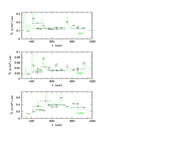
Figure 2: Filter spectra of example quasars: The three panels show quasars at different redshifts across the range addressed in this paper. The filter spectra are plotted with horizontal bars resembling the filter width and vertical bars for 1$\sigma$ flux errors. Due to variability repeated observations in B and R filters can show different flux levels for the same object. Variability is compensated for the construction of SEDs using R-band images which are available for every observing run. The best-fitting template spectra at indicated redshifts are plotted as grey lines.

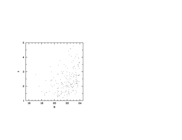
Figure 3: The present sample of 192 quasars: Distribution of redshifts over observed R-band magnitude. Notice that the sample has been truncated at $z=1.2$ and $R=24$.

3 The quasar catalogue

3.1 Sample definition

The quasar sample is extracted from the full survey catalogue purely on the basis of spectral information, thus deliberately ignoring morphological evidence. We believe that the classification of the ‘fuzzy spectra’ based on 17 filters, outlined below, allows to clearly differentiate between stars, galaxies and quasars, providing a safer separation between the object classes than morphological criteria. This is particularly important in the context of our interest in low-luminosity AGN which may well appear extended on a deep $R$-band image. Our purely spectroscopic classification approach ensures that the sample will not be heavily biased against such objects.

The sample finally used for all analyses in this paper is defined by limits in magnitude and redshift. Objects are selected to have a magnitude of $R>17$ to avoid the saturation regime in the individual frames, and $R<24$ which is where the completeness of the quasar identification has dropped below 30% (see Sect. 3.3). Since quasars show brightness variations, the sample selection will depend on the epoch of observation at the faint end. Here, we have used our R-band photometry from January 2000.

The sample is further limited to redshifts of $z>1.2$, since host galaxies may contribute significantly to the spectra at lower redshifts, where the 4000 $\mathrm{\AA}$-break is still contained within the filterset. Our templates currently contain only pure quasar and pure galaxy spectra, but no mixed templates with contributions from both. Therefore, identification and redshift estimation of low-luminosity quasars at $z<1.2$ is not straightforward at this point, and complicated completeness issues arise in the low-$z$ domain.

In order to ensure minimum contamination from non-active galaxies, we have set our probability threshold for an object to be classified as quasars quite high. As a result, we have eliminated many trustworthy low-luminosity AGN from the sample, but keep a well-controlled selection of higher-luminosity QSOs. We have chosen this conservative approach because we have not yet obtained spectroscopic confirmation redshifts for a sufficiently large sample to understand the selection function of low-luminosity Seyfert galaxies well enough.

The catalogue resulting from this selection contains 192 quasars between $z=1.2$ and $z=4.8$, with a median redshift of $\langle z\rangle=2.23$. Examples of quasar filter spectra are shown in Fig. 2, and the Hubble diagram for the full sample is presented in Fig. 3.

3.2 Classification and redshift estimation

The photometric measurements from 17 filters provide low-resolution spectra for each object which are analysed by a statistical technique for classification and redshift estimation based on spectral template matching (for details see Wolf et al. 2001a, ). Meanwhile, we have improved the template library for quasars by deriving it from the recent SDSS QSO template spectrum (vanden Berk et al., 2001), rather than from the earlier used pure emission line contour by Francis et al. (1991). This leads to a better detection and redshift estimation of quasars at $z<2.5$ where the ‘little blue bump’ may render the spectral shape between the prominent emission lines as quite different from the power-law which we assumed for the quasar templates previously. Since the CADIS work (Wolf et al., 1999), we have also learned that photometric redshifts for quasars are strongly influenced by flux variability.

Since the multi-colour observations were collected over a period of two years, and quasars as well as some stars show variability, it was necessary to correct for variability when constructing the 17-filter spectra for classification. For this purpose we used the $R$-band observations which are available for each observing epoch, allowing us to completely map the variability at least in this band. When constructing the SEDs of variable objects, we related the measurements of observed photometric band to the $R$-band magnitude obtained in the same observing run. As a result, the SEDs are not distorted by long-term magnitude changes. This variability correction works well only as long as flux variations are not accompanied by major changes in spectral shape. Furthermore, we also cannot account for short-term variability on a time scale of days, as within each observing run we have obtained only one $R$-band image.

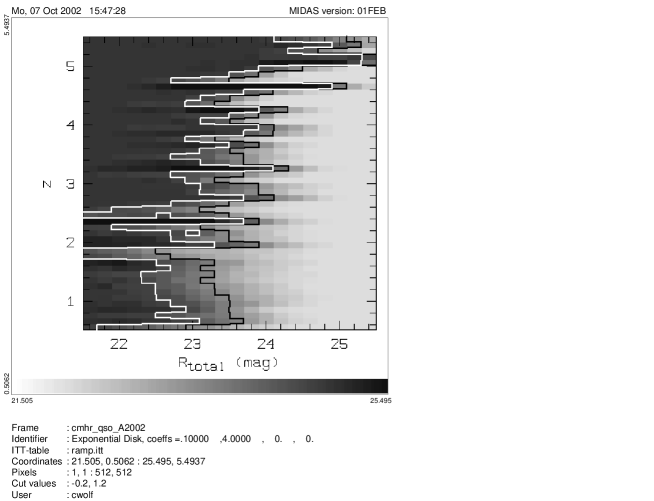
Figure 4: Completeness map for quasar selection and redshift estimation: Grey-scale and contour maps demonstrating how the fraction of quasars having successful redshift measurements depends on magnitude and redshift. Completeness levels are shown as a greyscale from 0 % (light grey) to 120 % (black). Contour lines are drawn for 90 % (white) and 50 % completeness (black). Values above 100 % occur when redshift aliasing creates local overdensities in the estimated $z$-distribution based on a flat underlying simulated distribution. See Sect. 3.3 for a more detailed discussion of the completeness correction.

3.3 Completeness correction

The subsequent analysis includes only objects with successful $z$ estimates. It is therefore critical to understand for which quasars the data permit such a classification. Given the photometric properties of the survey, we can produce mock catalogues of stars, galaxies and quasars with realistic photometric errors, and investigate the classification performance as a function of object type, redshift and magnitude. The 17-filter-spectra in the mock catalogues are constructed from the library templates, using the empirically derived observational error distributions. With this approach, the completeness of the classification and redshift estimation can be derived from Monte-Carlo simulations (see Wolf et al. 2001a, ). We implicitly assume that the spectral templates truly resemble observed objects, and if that is not the case, our simulation will be too optimistic.

In fact, we can test whether our completeness maps are realistic, given that within our fields and selection limits 12 broad-line AGN are known from spectroscopic observations in the CDFS (Hasinger 2002, priv. comm.; Szokoly et al, in prep.). The map predicts that 10 out of 12 objects should be identified, while in fact we recover 8. Two objects are missing from our sample although they lie in regions of high expected completeness: A QSO with broad absorption lines (BALs) at $z=3.6$ and a Sy-1 galaxy at $z=1.2$. The BAL QSO was misclassified as a star because of its unusually star-like colours. The Sy-1 galaxy resides just at our low redshift limit which we adopted to avoid incompleteness arising from the pure AGN spectra getting contaminated by host galaxy contributions. We conclude that on the whole our map is realistic, but that (a) rare QSOs with unusual colours could still escape our attention, and (b) right at the low-redshift limit the level of completeness might be reduced compared to our maps.

The product of the simulations for quasars is a completeness map (selection function), providing a formal probability $C(R,z,SED)$ that a quasar of given intrinsic properties is recovered, in bins of observed $R$-band magnitude and redshift. Our quasar template library contains a range of emission line strengths and a range in spectral indices or continuum colours. Effective spectral indices depend on redshift as the quasar continuum is not a pure power law. However, for a quasar at $z=2.0$ the range of template $B-I$ colours runs from about $+0.35$ to $+1.75$, corresponding roughly to power law indices of $\alpha=-1.66\ldots+0.4$. After we recognized that the simulated completeness depends very little on the spectral index, we collapsed the completeness function into $C(R,z)$ removing the explicit SED dependence (see Fig. 4).

At most redshifts, our classification algorithm is more than 90% complete for quasars with $R\la 23$. The contour line for 50% completeness ranges around $R\sim 23.5$. The redshift dependence of the completeness shows conspicuous oscillations above redshift 2, which are caused by the strong signature of the Lyman-$\alpha$ emission line migrating through the filter set and alternating between visibility in a medium-band filter and invisibility when it falls between two neighboring medium-band filters. Whenever the line is visible quasars can be identified to fainter levels due to its contrast.

At certain redshifts, the selection function reaches values above 100 %. This occurs when redshift aliasing creates local overdensities in the estimated $z$-distribution based on a flat underlying simulated distribution. Such ‘overcomplete’ regions are always accompanied by adjacent ‘undercomplete’ zones, so that the total number of objects is conserved.

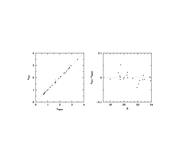
Figure 5: Spectroscopic vs. multi-colour redshifts: 22 QSOs from the COMBO-17 sample at $R<24$ have spectroscopic identifications. 21 of them were found to be QSOs at redshifts within $\pm 0.05$ of the multi-colour estimate, one of them is a White Dwarf/M dwarf-pair estimated at $z<1$.

3.4 Influence of limited redshift accuracy

For the analysis it is crucial to check to which extent the limited redshift accuracy of $\sigma_{z}\approx 0.03$ (as determined from the simulations) could affect inferences about luminosity functions. Two major aspects need to be explored, redshift aliasing and catastrophic mistakes, which are both irrelevant for interpreting well-exposed data from an aperture spectrograph, but could both play a role in our case:

1. Aliasing results from structures which are finer than the redshift resolution, violating the sampling theorem; it appears as fake structure on a scale that is typically slightly larger than the resolution. This effect is doubtlessly present in our data, as is also visible from the $z$-dependent oscillations in Fig. 4. In this paper, we avoid dealing with the problem altogether by only considering redshift bins of typically $\Delta z=0.6$, an order of magnitude larger than the resolution limit.

2. Catastrophic mistakes occur in certain regions of colour space where different interpretations can be assigned to the same colour vector and probabilistic assumptions are used to make a final redshift assignment. Obviously, a number of cases could lead to the assignment of a wrong redshift, but their effect on luminosity functions should be relatively small unless a major fraction of objects were affected. The only real impact would be in a situation in which many low-redshift objects of medium luminosity were wrongly assumed to reside at high redshift, boosting the abundance of the rare luminous quasars. We see no evidence for any such effect to be important.

A large-scale performance check of our spectrophotometric redshifts based on a substantial sample of spectroscopic redshifts is still pending. However, we have been able to test our classifications and redshifts against two samples of albeit limited sizes that have spectroscopic data. In the S11 field, the COMBO-17 sample overlaps at its bright end with the ‘2QZ’ quasar survey (Croom et al., 2001), and in the CDFS we found that a number of spectroscopically identified X-ray sources coincide with faint COMBO-17 AGN (Hasinger 2002, priv.comm.; Szokoly et al, in prep.). Fig. 5 shows a comparison of spectroscopic and multi-colour redshifts for all 22 objects from the COMBO-17 QSO sample with $R<24$ for which spectra exist. Only one of these 22 objects, classified as a QSO at $z\sim 0.6$ by COMBO-17 (i.e. outside the redshift range considered in this paper), was actually a misclassification; a 2QZ spectrum identified this object correctly as a White Dwarf/M dwarf-pair. The other 21 objects were found to be QSOs, and their redshifts agree all within $\pm 0.05$. This comparison suggests that the accuracy of COMBO-17 redshifts is certainly no worse than the assumed $\sigma_{z}=0.03$, and the rate of catastrophic mistakes is probably well below 10 %.

The CDFS contains several further faint Seyfert galaxies, particularly at $z<1$, most of which were recently identified as optical counterparts to faint X-ray sources. These are very challenging objects for the multi-colour redshift estimation, as their host galaxies will contribute significantly to their overall SED. Clearly, more work is needed to tackle these objects, which are therefore explicitly excluded from the scope of this paper.

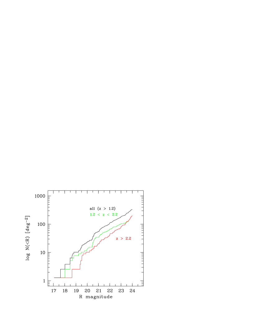
Figure 6: Cumulative surface density of AGN as a function of $R$ band magnitude, corrected for Galactic extinction.

Table 3: Tabulated AGN number counts as a function of $R$ band magnitude. The 2nd and 4th column give the actual numbers of objects in the current COMBO-17 sample (within 0.78 deg²), while the 3rd and 5th column give incompleteness-corrected surface densities per deg².

	$z>1.2$		$z>2.2$
$R$	$n$	${\cal N}(<R)$	$n$	${\cal N}(<R)$
24.0	192	336.5	101	201.7
23.0	139	183.2	60	79.5
22.0	86	107.7	33	41.8
21.0	43	55.1	16	20.5
20.0	18	23.1	8	10.3
19.0	8	10.3	2	2.6
18.0	2	2.6	1	1.3

4 Number counts

From the AGN sample and the completeness map described above it is straightforward to compute surface densities as a function of apparent magnitude, using the relation

$${\cal N}(<R)\>=\>\sum_{i}\frac{1}{A_{i}}\>=\>\frac{1}{A_{0}}\,\sum_{i}\frac{1}{C(R_{i},z_{i})}$$ (1)

where the summation runs over all AGN brighter than $R$. $A_{0}$ is the formal total survey area of 0.78 deg²; multiplying this with the value of the completeness map $C(R_{i},z_{i})$ for object $i$ yields the estimated ‘effective survey area’ $A_{i}$ for that particular source. In other words, the decreased probability of detecting very faint AGN, particularly relevant for certain redshift ranges, is simply interpreted as being equivalent to a reduced survey area for such objects.

Results are shown in Fig. 6 and listed in Table 3. Besides the full sample of all $z>1.2$ AGN, we also show the number counts for subsamples split at $z<2.2$ and $z>2.2$, the typical high-redshift limit of UV excess surveys. The two subsamples show very different trends towards the faint limit: While the low-$z$ objects dominate at brighter magnitudes, their surface density increases only slowly with decreasing flux level. On the other hand, the cumulative number of AGN with $z>2.2$ is a strong function of magnitude, and quite well described by a power law ${\cal N}(<R)\propto R^{-0.31}$, corresponding to a power law index of $-1.75$ for the differential number-flux relation. Towards the faint end it even seems as if the slope might be increasing, but this is not formally significant. Nevertheless, for $R>23$ it is clear that high-redshift AGN with $z>2.2$ become the dominant population.

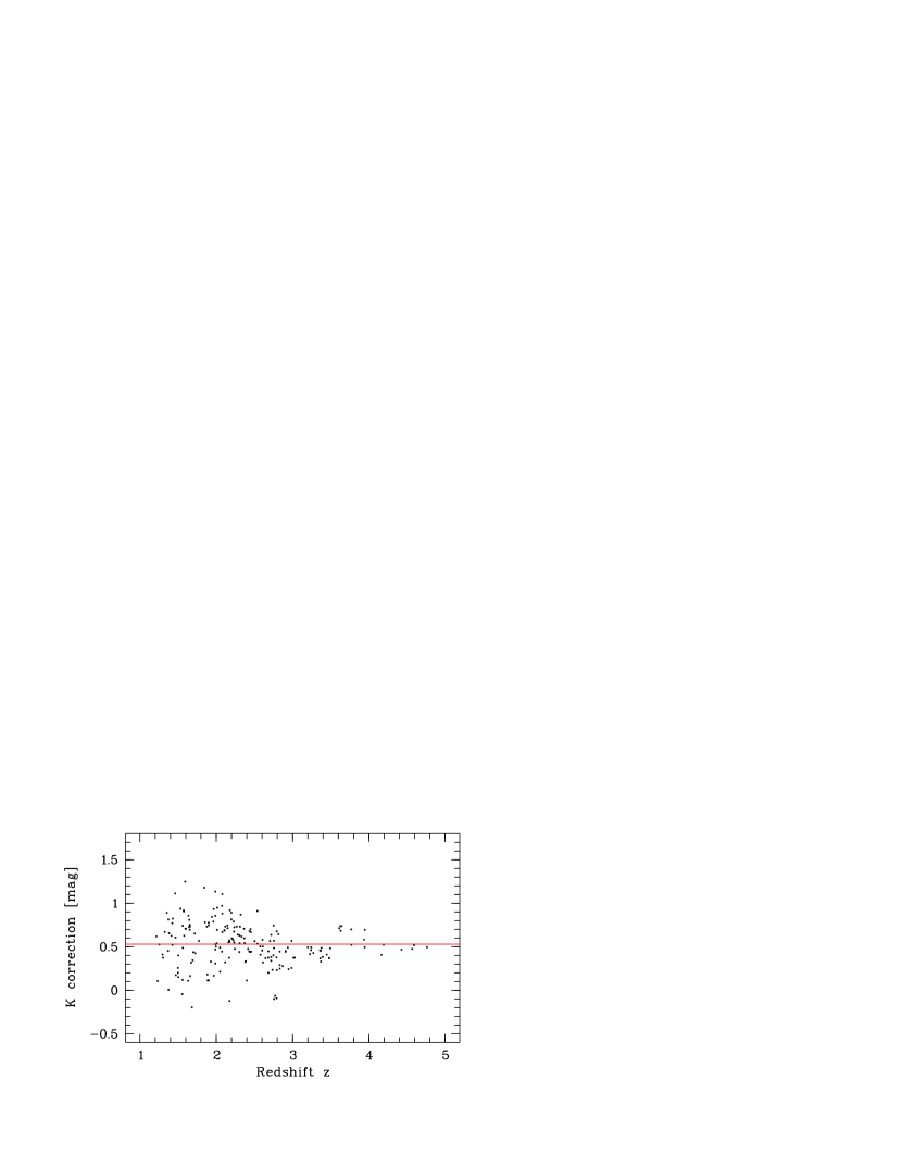
Figure 7: Derivation of the internal K correction used in this paper: Each point corresponds to one individual AGN measurement based on the SED fits within COMBO-17. The horizontal line is a linear fit, allowing to predict luminosities at 145 nm with an accuracy of 0.24 mag.

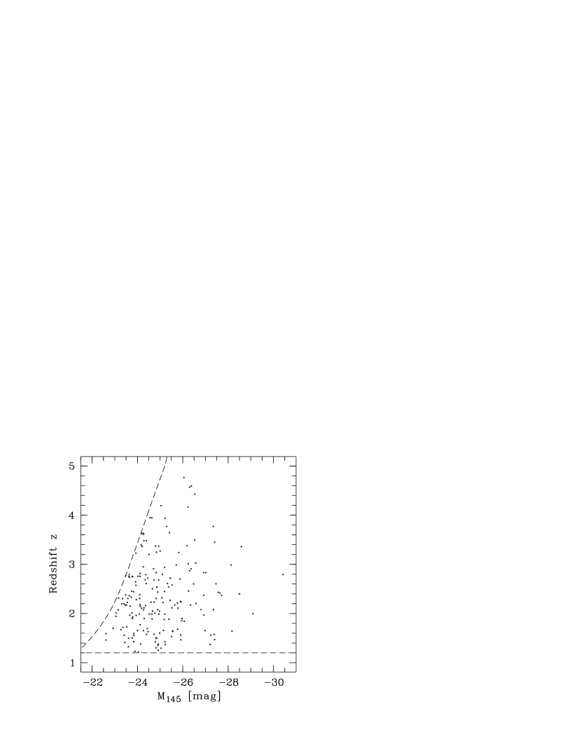
Figure 8: Distribution of the input sample over absolute magnitudes and redshifts: The dashed lines indicate the imposed sample limits of $z>1.2$ and $R<24$.

5 Estimation of rest frame luminosities

For each object in the sample we have individual SEDs from the 17-filter spectrophotometry at our disposal. In order to derive absolute magnitudes for the subsequent analysis, we decided to tie all luminosities to the UV continuum level at $\lambda_{\mathrm{rest}}=145$ nm. This was realised by integrating the best-fitting redshifted template over a synthetic narrow rectangular passband at 143 nm–147 nm, thus avoiding the Si iv/O iv emission line at 140 nm. This procedure enabled us to directly measure rest-frame luminosities over a redshift range $1.4\la z\la 5$ without any need for extrapolation.

While such individually determined luminosities may suffer less from biases arising in uncertain assumptions on AGN spectral energy distributions than some previous samples, they considerably complicate the statistical exploitation. Although most of our objects are detected in all or nearly all of the 17 filter bands, the sample is presently defined only in the $R$-band: (1) The flux limit is homogeneously truncated at $R<24$. (2) The completeness map has the $R$ band magnitude as one of its two independent parameters. It is also assumed in the algorithms used for luminosity function estimation that the survey is defined by just one flux limit. We have therefore explored whether it is possible to estimate absolute UV magnitudes $M_{145}$ from the measured $R$ band flux, using a modified but basically traditional $K$ correction approach.

For this purpose we computed for each quasar its absolute magnitude directly from the distance modulus, $M_{0}=R-(m-M)$, equivalent to assuming a $K$ correction for a power-law spectrum with slope $\alpha=-1$. We then plotted the differences $\Delta M$ between $M_{0}$ and $M_{145}$ (the spectrophotometric estimates) against source redshift; this is shown as the distribution of points in Fig. 7. This plot shows that at least at redshifts $z\ga 2$ there is a well-defined relation between $z$ and $\Delta M$. When fitting a constant line through these points, as shown in Fig. 7, we get an overall rms scatter of 0.24 mag (0.13 mag for $z>2.2$ and 0.26 mag for $z<2.2$), which can only insignificantly be improved by fitting e.g. a low-order polynomial. This line defines then an empirical correction relation $K(z)$, so that for the redshift range of interest in this paper we can use $R$ band magnitudes to estimate $M_{145}$ with an accuracy of 0.24 mag, even without using any SED information.

Most earlier studies of the optical AGN luminosity function, especially those focussing on lower redshifts, have expressed their results in terms of blue magnitudes $M_{B}$. In order to facilitate a statistical comparison, we obtained a crude estimate for the offset $M_{B}-M_{145}$ by repeating the above procedure for the rest-frame $B$ band. Note that for all $z>1.2$ objects this involves a good deal of extrapolation, and the diagram corresponding to Fig. 7 shows more than 0.6 mag of scatter around the mean trend. Nevertheless, the offset of 1.75 mag thus determined is actually identical (to 0.01 mag) to the result when the same quantity is measured in the mean quasar energy distribution of Elvis et al. (1994). In conclusion this means that all quoted absolute magnitudes $M_{145}$ can be converted into $M_{B}$ using the relation $M_{B}=M_{145}+1.75$.

In the subsequent analysis we use two sets of cosmological parameters, an Einstein-de Sitter universe with $H_{0}=50$ km s^-1 Mpc^-1, $\Omega_{m}=1.0$ and $\Omega_{\Lambda}=0$, and a flat ‘concordance model’ with $H_{0}=65$ km s^-1 Mpc^-1, $\Omega_{m}=0.3$ and $\Omega_{\Lambda}=0.7$. While the former is now physically almost obsolete, it still has some relevance as a ‘yardstick’ model, as most earlier studies of AGN evolution were expressed preferentially in these terms. Actually we found that the results change very little when switching between the two models, except for small shifts in both axes, and our displayed results always refer to the ‘concordance universe’ unless explicitly stated otherwise. Figure 8 shows the distribution of absolute magnitudes vs. redshift for the entire AGN sample. In terms of the conventional (if arbitrary) distinction between high-luminosity quasars and low-luminosity Seyferts around $M_{B}\simeq-23$, our sample covers just the region close to this dividing line. It is therefore the first optically selected AGN sample of substantial size to probe this important regime of nuclear activity in galaxies. It also matches very well the luminosity range covered by low-$z$ AGN surveys that provide a $z\simeq 0$ reference (e.g., Köhler et al., 1997).

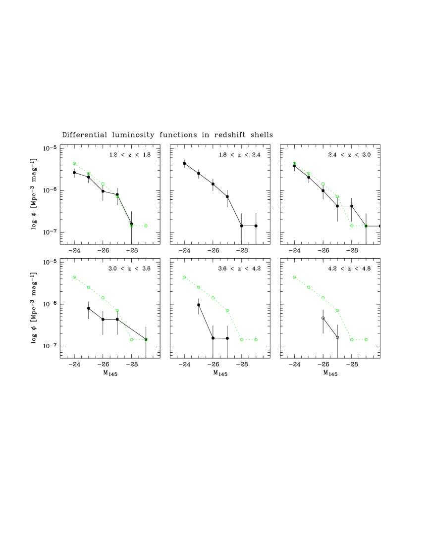
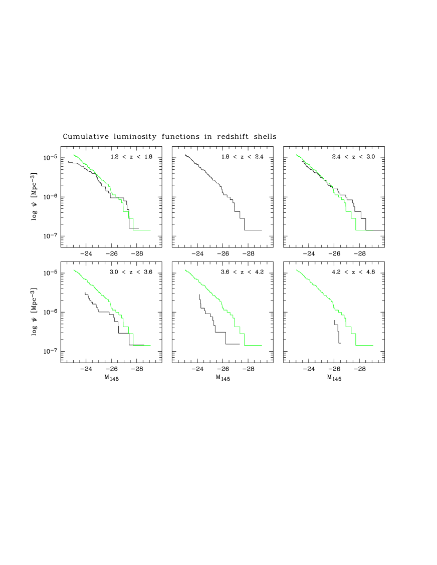
Figure 9: (a) Binned differential luminosity functions for six non-overlapping redshift shells. Only luminosity bins completely covered by the sample are shown. In addition to the data with Poissonian error bars, each panel features the $1.8<z<2.4$ luminosity function as reference. (b) Cumulative luminosity functions for the same redshift shells.

Table 4: Tabulated binned AGN luminosity function.

		1.2–1.8		1.8–2.4		2.4–3.0		3.0–3.6		3.6–4.2		4.2–4.8
$M_{145}$	$M_{B}$	$n$	$\log\phi$	$n$	$\log\phi$	$n$	$\log\phi$	$n$	$\log\phi$	$n$	$\log\phi$	$n$	$\log\phi$
$-$23.0	$-$21.2	7	$-$5.78	9	$-$5.53	0		0		0		0
$-$24.0	$-$22.2	16	$-$5.58	22	$-$5.36	17	$-$5.42	5	$-$5.85	3	$-$6.02	0
$-$25.0	$-$23.2	13	$-$5.69	17	$-$5.60	14	$-$5.69	5	$-$6.10	6	$-$6.02	0
$-$26.0	$-$24.2	6	$-$6.02	10	$-$5.85	7	$-$6.01	3	$-$6.36	1	$-$6.81	3	$-$6.33
$-$27.0	$-$25.2	5	$-$6.10	5	$-$6.15	3	$-$6.38	3	$-$6.36	1	$-$6.81	1	$-$6.79
$-$28.0	$-$26.2	1	$-$6.80	1	$-$6.85	3	$-$6.38	0		0		0

6 Evolution of the AGN luminosity function

6.1 Non-parametric estimates

6.1.1 Method of computation

We employ the usual $1/V_{\mathrm{max}}$ estimator Schmidt (1968) to give the space density contributions of individual objects. Luminosity functions are then readily obtained by forming the appropriate sums: Denoting the luminosity-binned differential LF as $\phi(M)$ and the cumulative LF as $\psi(M)$ we have

$$\phi(M,z) = \sum_{M-\Delta M}^{M+\Delta M}\>\sum_{z-\Delta z}^{z+\Delta z}\frac{1}{V_{i}}\>,$$ (2)

$$\psi(M,z) = \sum_{-\infty}^{M}\sum_{z-\Delta z}^{z+\Delta z}\frac{1}{V_{i}}$$

where each value of $V_{i}$ is the total comoving volume within which object $i$ would still be included in the sample. The value of $V_{i}$ follows from integrating the survey selection function $C(R,z)$, introduced in Sect. 3.3, over all relevant redshifts:

$$V_{i}(R,z)=A_{0}\int_{z}^{z_{\mathrm{max}}}{C(R,z)\frac{dV}{dz}dz}$$ (3)

(cf. Wisotzki, 1998) where $A_{0}$ is again the formal total survey area, $A_{0}=0.78$ deg² in the present case. The assigned error bars are based purely on Poissonian shot noise due to the limited AGN counts within each bin, i.e. we ignored errors in magnitude or redshift estimation. The error bars for a given sum are then given by

$$\sigma_{\phi}=\sqrt{\sum_{i}1/V_{i}^{2}(M,z)}.$$ (4)

It is well known that binned estimates of luminosity functions suffer from a number of biases. In particular, two effects are worth being recalled, both of which can be seen as two different variants of Malmquist bias and lead to the observed LF appearing flatter than the intrinsic one:

• Binning in magnitude and a steep LF create a positive bias in the derived space densities, due to a shift in effective bin centres towards lower luminosities.

• Differential evolution within redshift shells leads to an overestimation of space densities where the LF is steep.

While the first effect is absent in the cumulative LF representation, the latter is unavoidable as long as no model assumptions for the evolution of space densities are made. It should thus be kept in mind that the nonparametric LFs discussed in the following section do not necessarily show the data ‘as they are’, but just form the most conventional way of presenting luminosity function data.

6.1.2 Results

Inside the redshift interval $1.2<z<4.8$ covered by the COMBO-17 sample we defined six redshift shells of equal sizes to trace the evolution of the QLF. Figure 9 gives a synopsis of the results; for the benefit of interested readers who wish to use our data for their own computations we present the tabulated binned LFs in Table 4. This table shows also how many objects contributed to each bin. The numbers given in this table show that the differences between adjacent redshift shells are not huge, i.e. evolution is relatively moderate over this redshift range. We therefore have deviated from the usual practice to plot all LFs into one frame, as any real trend would be very hard to discern in such a diagram. Instead, we created individual subpanels for each redshift shell and plot each luminosity function separately, but together with the $1.8<z<2.4$ LF taken as a reference. This visualisation shows that the measured values of the LF are below the corresponding reference values in nearly all data points. In other words, we detect an unambiguous maximum in the comoving AGN space density near these redshifts, and a significant drop towards both lower and higher $z$. The existence of such a maximum becomes even clearer in Fig. 11 where integrated space density at given lower bound in luminosity (taken directly from the cumulative LFs in each redshift shell) is plotted directly against $z$. We return to a more detailed discussion of the evolution of space densities and LF shape properties below.

6.2 Parametric analysis of the luminosity function

6.2.1 Ansatz

Within certain bounds and accuracy limits, an observed luminosity function can usually be described quite well by some simple analytic expression, allowing one to compress the results into a few well-determined numbers, with the positive side effect that the above mentioned Malmquist-type biases due to data binning can be avoided by obtaining luminosity function and evolution parameters simultaneously from an observed sample. This was first demonstrated by Marshall et al. (1983) for a very simple power law model of the evolving QLF. Since the parametric forms employed for the analysis in this paper are somewhat non-standard, we use the following paragraphs to spell out the adopted ansatz.

Shape of the luminosity function:

The most common analytic description of the QLF is a double power law, involving a bright-end slope $\gamma_{1}$, a faint-end slope $\gamma_{2}$, and a smooth turnover at a characteristic ‘break’ luminosity $M^{\star}$. We have explored this ansatz and decided not to use it for the present sample, mainly because we fail to identify a well-defined break luminosity in the data. Direct fitting of a double power law LF to any of the redshift shells subsamples shows that $M^{\star}$ is a very ill-constrained quantity that often takes a value outside the luminosity range covered by the sample; furthermore, even minor modifications in the subsample definition can cause major changes in $M^{\star}$. Since the luminosity functions in Fig. 9 undoubtedly show some indication of curvature, we decided to parametrise the LF, at given $z$, as a polynomial in $M_{145}$:

$$\log\phi\>=\>\sum_{i=0}^{n}\>A_{i}\,\mu^{i}\>.$$ (5)

where $\mu=M_{145}-M^{\star}$ and $M^{\star}$ is a constant which can be chosen freely but may also contain the effects of luminosity evolution (see below). In this representation, $A_{0}=\log\phi_{0}$ is the space density normalisation at $M_{145}=M^{\star}$, which in our case has mostly been set to $M^{\star}=-25$ (roughly corresponding to $M_{B}=-23.25$). For $n=1$, the LF is a single power law with slope $\gamma=-2.5A_{1}-1$.

Evolution parameters:

The last decade has seen a sometimes hot debate over the question whether ‘pure luminosity’ or ‘pure density’ evolution were more appropriate. We have implemented both parametrisations as well as mixed forms. As independent variable we use

$$\zeta\>=\>\log\left(\frac{1+z}{1+z_{\mathrm{ref}}}\right)$$ (6)

which vanishes for $z=z_{\mathrm{ref}}$. For our analysis we avoid extrapolating to redshifts outside the sample definition interval and adopt $z_{\mathrm{ref}}=2$. Pure density evolution is then expressed as polynomial expansion of the space density normalisation:

$$\log\phi_{0}(z)\>=\>\sum_{j=0}^{m_{D}}\>C_{j}\,\zeta^{j}\>.$$ (7)

For $m_{D}=1$, the parameter $C_{1}$ is equal to the density evolution index $k_{D}$ used in several earlier analyses.

On the other hand, pure luminosity evolution involves a redefinition of the LF parameter $M^{\star}$:

$$M^{\star}(z)\>=\>M^{\star}(\zeta=0)\,+\,\sum_{j=1}^{m_{L}}\>B_{j}\,\zeta^{j}\>.$$ (8)

(Note that unlike for a ‘broken power law’, $M^{\star}(\zeta=0)$ is here an arbitrary constant and not a free fit parameter.) Again, the case of $m_{L}=1$ corresponds to a standard form already used by several previous authors, $M^{\star}(z)\propto(1+z)^{k_{L}}$. In this case the luminosity evolution index is $k_{L}=0.4B_{1}$.

Fitting method:

We followed a maximum likelihood approach (Marshall et al., 1983) to search for optimal parameter combinations, using a modified downhill-simplex minimisation scheme (Press et al., 1992). Several goodness-of-fit tests were applied to check whether the best-fit model was adequate. These included one- and two-dimensional Kolmogorov-Smirnov tests for the distributions over the $(M,z)$ plane, as well as a $\chi^{2}$ test that directly compares observed and predicted numbers of AGN in redshift/luminosity bins. A fit was considered satisfactory only when it passed all of the statistical tests with a probability for the validity of the null hypothesis of $>10$ %. This highly conservative approach ensures that the missing distribution-free properties of the KS test (see Wisotzki 1998 for discussion on Lilliefors et al., 1968) can be neglected.

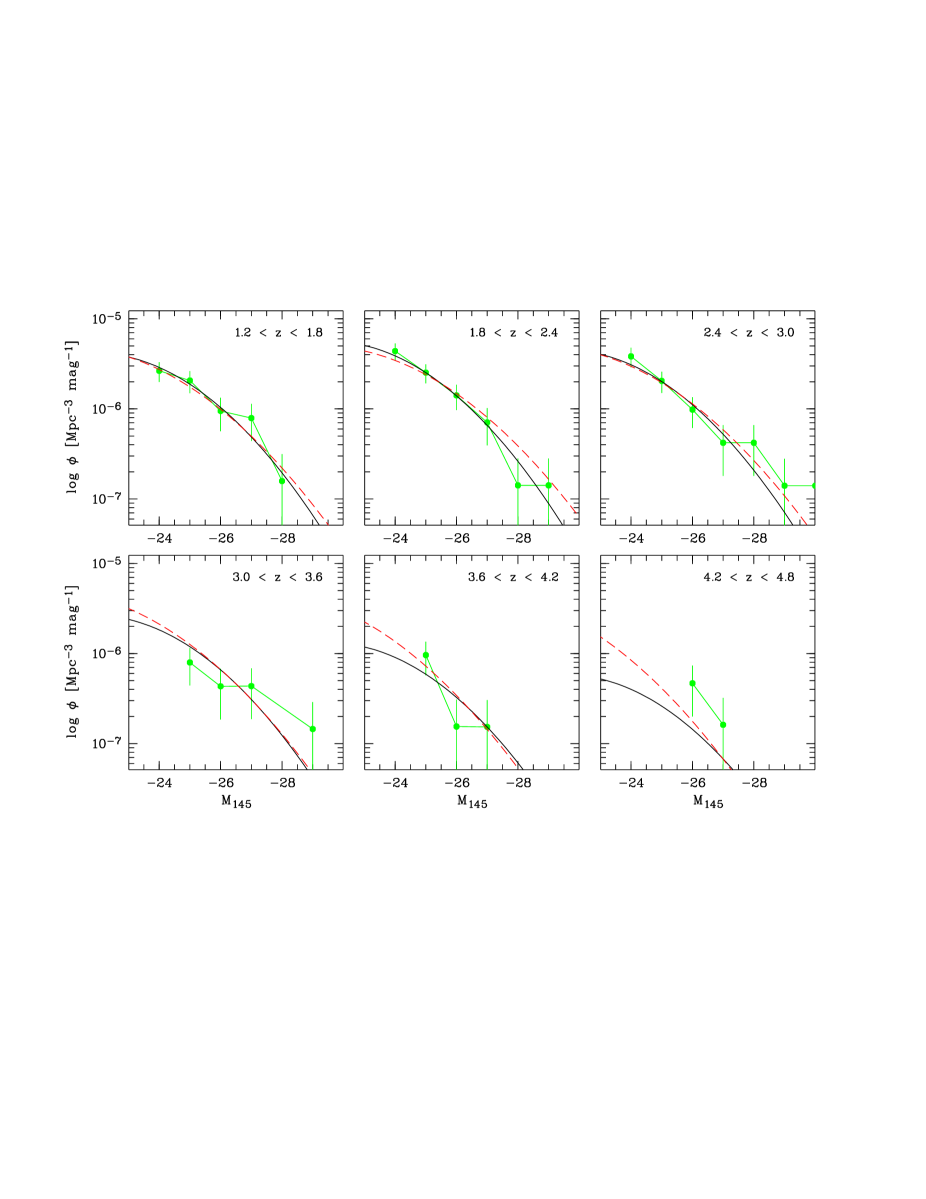
Figure 10: Best-fit parametric representations of the evolving luminosity function, plotted against the binned LF data from Fig. 9(a). The density evolution model is shown by the solid, the luminosity evolution model by the dashed lines.

Figure 11: Evolution of comoving AGN space density with redshift, for different lower luminosity limits, and for two cosmological models. Filled circles: $M_{145}<-24$; open circles: $M_{145}<-25$; filled squares: $M_{145}<-26$; open triangles: $M_{145}<-27$. The corresponding curves are integrated from the best-fit PDE models.

6.2.2 Results

Starting with the simplest possible luminosity function, we found that a single power law LF as an overall shape model had to be rejected as there is weak but significant curvature in the LF, especially for the lower redshift ranges, $z\la 2.4$. But already a 2nd order poynomial gives a statistically adequate description of the LF at all redshifts. Note that this form involves one free parameter less than the case of a double power law LF.

Table 5: Coefficients of the best-fit analytic models describing the luminosity function and its evolution as either PDE or PLE. For details on the notation see text.

Model	$A_{0}$	$A_{1}$	$A_{2}$	$M^{\star}_{145}(0)$	$C_{1}$	$C_{2}$	$B_{1}$	$B_{2}$	$B_{3}$
PDE	$-$5.600	0.2221	$-$0.03536	$-$25	0.3599	$-$15.574
PLE	$-$5.620	0.1845	$-$0.02652	$-$25			1.3455	$-$80.845	127.32

As a first evolution mode we explored pure density evolution (PDE). A global PDE fit over the entire redshift range $1.2<z<4.8$ was achieved with again just a 2nd-order polynomial to reproduce the maximum of comoving space density around $z\simeq 2$. Alternatively, the sample can be described equally well by pure luminosity evolution (PLE), albeit requiring one more parameter than PDE. Our best-fit PLE model features a 3rd order polynomial for the function $M^{\star}(z)$. The predicted parametric luminosity functions are compared with the binned nonparametric estimates in Fig. 10. Both fits provide excellent descriptions of the data, with goodness-of-fit probabilities of $p>50$ % for all statistical tests (see Tab. 5 for best-fit models). The differences between PDE and PLE luminosity functions become significant only outside the luminosity range sampled by the COMBO-17 data.

In Fig. 11 we show the cumulative luminosity function as a function of redshift, for different limiting luminosities, again together with the corresponding nonparametric estimates. For simplicity, only the PDE result is plotted. Since the fit is presently unconstrained below $z=1.2$, we have marked the extrapolation into this region by a dotted line. The fit is completely consistent with the individual binned datapoints.

7 Discussion

7.1 The maximum of AGN activity

The dominant feature in Fig. 11 is the peak of comoving AGN space densities around $z\simeq 2$. Although its existence was beyond doubt for a long time, rarely has it been possible to locate the maximum within a single survey. UV excess-selected samples typically reach up to $z=2$–2.5 and mainly trace the rise at low $z$; conversely, most dedicated high-redshift surveys start being effective only beyond $z\simeq 3$ and just show the decreasing branch. The COMBO-17 sample combines properties of both search techniques and covers enough redshift range that the peak of AGN activity is clearly bracketed. The PDE and PLE fits both place the maximum at a redshift of $z_{\mathrm{max}}=2.1$.

An important issue for the astrophysical interpretation of AGN evolution is a possible luminosity dependence of the peak location. For example, in hierarchical structure formation one expects objects of higher mass objects to form later, which in a simple scenario of correlated masses and luminosities should manifest in high-$L$ AGN to show a peak at lower redshifts. This is certainly not the case in our data; on the contrary, one might be tempted to speculate from Fig. 11 that there could be a gradual shift of the maximum towards higher redshifts when the luminosity limit is increased.

We have tried to model such a trend by including explicit luminosity-dependent density evolution parameters, e.g. in the form of a linear dependency between absolute magnitude and $z_{\mathrm{max}}$. While the data are statistically consistent with a moderate shift, the best-fit model was always very close to simple PDE, despite the additional degrees of freedom. We conclude that there is no indication for a dramatic difference between the space density peaks of AGN of different luminosities, within the range covered by COMBO-17.

A similar but much stronger effect, a shift of maximum space density towards lower redshift for very low luminosity AGN, has recently been reported for deep X-ray selected samples (Cowie et al., 2003; Hasinger et al., 2003). While a detailed comparison between the properties of X-ray and optically selected AGN samples is beyond the scope of this paper, we just note two aspects which need to be taken into account: Firstly, the new X-ray selected samples probe even much deeper than COMBO-17 into the population of AGN with very low luminosities. Assuming an Elvis et al. (1994) AGN spectrum, our low-luminosity limit of around $M_{145}=-23$ corresponds to a 2–8 keV luminosity of roughly $L_{x}\simeq 43.6$; this is just the point where the difference becomes visible, according to Cowie et al. and Hasinger et al.

But secondly, the X-ray and optical luminosity functions of high-redshift AGN also show significant dissimilarities. In particular, the X-ray LF of type 1 (broad-line) AGN near $\log L_{x}\simeq 44$ is very nearly constant (cf. Cowie et al.; Hasinger et al.), while the optical LF around the corresponding $M_{145}\simeq-24.6$ is still significantly rising (cf. Fig. 9). This may be indicative of different spectral shapes between low- and high-luminosity, or between low- and high-redshift AGN, all leading to nontrivial $L_{x}$ to $M_{145}$ conversions. Thus, while on one hand our $R<24$ sample may still be not quite deep enough to see similar effects as found in the X-ray domain, it is not even obvious that exactly the same effects should be expected for a yet deeper sample.

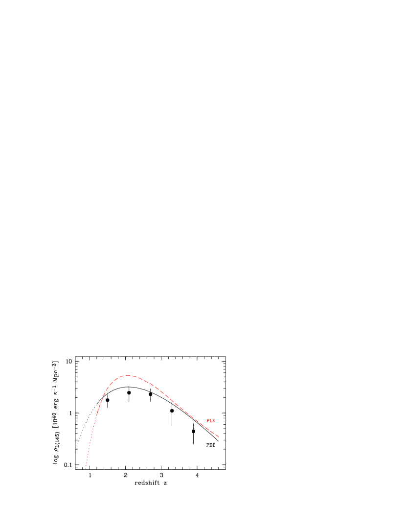
Figure 12: Integrated UV luminosity density $\varrho_{L(145)}$ as a function of redshift, estimated from the cumulative LF (data points) and for both PDE (solid) and PLE (dashed) models. Below $z=1.2$ the relations are extrapolated (dotted lines). The discrepancy between PLE and PDE around the maximum is entirely due to the differences in the bright-end slope of the luminosity function.

7.2 Evolution of the AGN luminosity density

The contribution of AGN to the metagalactic radiation field is probably relevant for several wavebands. Recent satellite missions were very successful in resolving the extragalactic X-ray background as mainly due to distant low-luminosity AGN (e.g. Miyaji et al., 2000). Likewise, the diffuse ionising UV background is believed to be strongly influenced by AGN, but a quantitative synthesis still relies on several assumptions and extrapolations. One of the principal uncertainties has always been the shape of the low-luminosity end of the AGN luminosity function. In order to estimate the AGN luminosity density $\varrho_{L}(z)$, one has to evaluate the integral

$$\varrho_{L}(z)=\int_{L}L\,\phi(L,z)\,dL\>.$$ (9)

The integral diverges only for a luminosity function slope $\gamma<-2$, but the relative contributions of AGN at different luminosity levels depend critically on the overall shape of the LF.

The COMBO-17 AGN sample goes deep enough that, for the first time, the quantity $L\,\phi$ can be safely integrated without depending on heavy extrapolation into the unobserved range. We have computed both binned nonparametric as well as parametric estimates of $\varrho_{L}(z)$, which we show in Fig. 12. We present the monochromatic luminosity density $\varrho_{L(145)}$, based on the value of $\lambda L_{\lambda}$ evaluated at $\lambda=145$ nm (which in turn is directly derived from $M_{145}$). Assuming a typical QSO spectrum such as the one given by Elvis et al. (1994), the quantity $\varrho_{L(145)}$ can also be extrapolated into a frequency-integrated luminosity density. Since we are particularly interested in the AGN contribution to the cosmic production of hydrogen-ionising photons, we provide the necessary conversion:

$$L_{\lambda<91.2\,\mathrm{nm}}\>=\>1.45\times\lambda L_{\lambda=145\,\mathrm{nm}}\>.$$ (10)

Notice that we have individual SED information on each of the COMBO-17 objects, which in principle could be used to derive a more accurate estimate of $L_{\mathrm{ion}}$. This will be done in a later paper dedicated to the synthesis of the UV background from the COMBO-17 AGN sample.

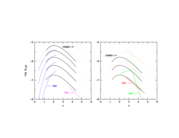
Figure 13: Best-fitting parametric models of quasar space density in comparison: Solid lines are constrained by respective surveys and dashed lines are extrapolations to fainter luminosities. Left: COMBO-17 with 2QZ and SDSS (Fan et al.), at luminosities of $M_{145}<[-28\ldots-24]$. The apparent disagreement of COMBO-17 with 2QZ at brightest luminosities should not be taken seriously as the curves show the best-fitting model and not actual LF data. Right: COMBO-17 with WHO and SSG, at luminosities of $M_{145}<[-28,-27,-26]$.

For the nonparametric estimates we computed $\varrho_{L}$ by summing over the luminosity-weighted inverse volumes $L/V_{i}$ up to the survey limit; the resulting numbers should set lower limits to the full integral over all luminosities. The two adopted parametric forms of PDE and PLE can be directly integrated to provide smooth functions $\varrho_{L}(z)$. It is worth noting that the integral effectively converges within the COMBO-17 survey limits; the difference between setting the low-luminosity integration boundary at $M_{145}=-23$ (approximately the COMBO-17 limit) and at $M_{145}=-10$ (or $L=0$) is only 2 %. In other words, the constraints on the faint end of the AGN luminosity function from COMBO-17 are already sufficient to estimate the total UV radiative output from AGN. This is also illustrated by the relatively good agreement in Fig. 12 between the binned estimates (which, as said above, are formally just lower limits to $\varrho_{L}$) and the PDE model.

On the other hand, the flat slope of the LF makes the contribution of brighter AGN to $\varrho_{L(145)}$ anything but negligible. In fact, the inclusion or exclusion of individual high-luminosity objects makes a noticeable difference for the binned estimate. (This is much less so for the parametric estimates, because of the uniform weighting inherent in the maximum likelihood procedure.) The importance of higher luminosity objects becomes particularly apparent when comparing the PDE- and PLE-derived relations. The substantial and significant differences seen in Fig. 12 are not due to faint-end extrapolation effects, but entirely originate in the much flatter LF slope of the PLE model at brighter magnitudes, already documented in Fig. 10 above. We reiterate that these discrepancies are due to the limited power of the COMBO-17 dataset to discriminate between evolution models. They will be resolved as soon as constraints from other, brighter AGN surveys are combined with the COMBO-17 sample.

7.3 Comparison with other surveys

7.3.1 Redshift $1.5<z<4.5$

In terms of the luminosity range, our quasar sample pushes to fainter limits than any previous survey. Our targets mainly have observed magnitudes of $R=20\ldots 24$, while previous surveys either observed down to $R\la 20$ if they derived luminosity functions, or observed to $R\la 22.5$ but produced object lists which did not constrain the luminosity functions very much further. Therefore, this work enters a new regime of studying low-luminosity AGN at intermediate to high redshifts.

A first attempt to conduct an AGN survey with a strategy similar to COMBO-17 was performed, albeit on a much smaller scale, in the course of the CADIS survey (Wolf et al. 1999), where a sample of 12 QSOs at $z>2$ and $R<22$ was identified within an area of 250 arcmin². Their resulting surface density is twice as high as for COMBO-17, but because of the small sample size, the results of CADIS and COMBO-17 are still formally compatible. The discrepancy underlines, however, the importance of cosmic variance and hence the need to obtain large samples.

Major previous work producing luminosity functions include the 2QZ at $z\la 2.3$ (Boyle et al., 2000), the work by WHO at $2.0<z<4.5$, and by SSG at $z>2.7$ as well as the results from the high-redshift SDSS sample at $z>3.6$ by Fan et al. (2001). As we have little overlap with all these previous surveys in luminosity, we cannot test directly to what extent our and their luminosity functions coincide. However, at the bright end our LF is completely consistent with an extrapolation of the SDSS-based LF given by Fan et al., with similar slope and similar normalisation. SSG cover a slightly wider range of redshifts down to $z=2.7$, but there still is not much overlap, so as before we need to extrapolate. The SSG slope is steeper than that of Fan et al., so that the SSG prediction for our regime is even further above the COMBO-17 results.

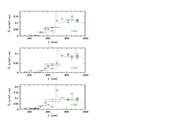
Figure 14: Filter spectra of the three $z>4.5$ COMBO-17 quasars in the present sample. See Fig. 2 for interpretation of the symbols.

On the lower-redshift side, our results smoothly connect to the 2QZ results. At intermediate redshift again, WHO used a broken power-law to characterize the QLF, where they found a steep end slope of $\alpha=-1.67$ and a faint end slope of $\beta=-0.45$, which is mostly constrained by the probably non-optimal assumption of a broken power-law. The bright end of our LF varies around 0.4 to 0.7 in their units and can be considered consistent with the WHO faint-end.

7.3.2 Quasars at $z>4.5$

The redshift range above 4.5 is subject to several studies from dedicated surveys to find faint high-redshift quasars. At highest luminosities the SDSS has delivered samples of six objects in 180 $\mbox{deg}^{2}$ at $i^{*}<20$ (Fan et al., 2001) and 29 objects in $\sim 700\leavevmode\nobreak\ \mbox{deg}^{2}$ at $i^{*}<20.5$ (Andersen et al., 2001). Medium-deep surveys across cover smaller areas, among which the BTC40 has so far reported two $z>4.5$ QSOs at $I<21.5$ across 36 $\mbox{deg}^{2}$ and still have a list of fainter candidates at $I\la 22$ to follow up (Monier et al., 2002). The Oxford-Dartmouth Thirty Degree Survey (ODT) also aims at finding $z>4.5$ quasars down to $I<22$ on 30 $\mbox{deg}^{2}$ (Dalton, priv. comm.). Monier et al. (2002) demonstrate the consistency of their currently available small numbers with the SDSS result and predict on the basis of the SDSS-LF a surface density of 0.026 $/\mbox{deg}^{2}$ at $z>4.5\ldots 5.0$ and $I<19.9$, and much less at $z>5$.

COMBO-17 covers only 0.78 $\mbox{deg}^{2}$ currently, but reaches a bit deeper. An extrapolation of the SDSS luminosity function suggests we should find 2.0 quasars per $\mbox{deg}^{2}$ at $I<23$ and $z>4.5$. Our observation of some curvature in the fainter domain of the luminosity function reduces that prediction to $\approx 1.25/\mbox{deg}^{2}$, so one or two objects is the total number to be expected in the COMBO-17 dataset.

The present sample contains three objects at $z>4.5$, all in the S11 field (see Fig. 14 for filter spectra). They all have $I<22$, although our selection should be complete to $I<23$. Basically, this observation is statistically consistent with an extrapolation of both the SDSS LF and our own. As we can not draw strong conclusions about the cosmic abundance of these objects from COMBO-17, they have been excluded from the LF results presented above.

Table 6: Predicted AGN surface densities, based on (partly extrapolated) COMBO-17 results. Each field gives the cumulative AGN number per deg², brighter than $R$ and with redshift greater than $z$, as derived from the two simple evolution models discussed in this paper.

Magnitude	$N(z>2)$		$N(z>3)$		$N(z>4)$		$N(z>5)$
	PDE	PLE	PDE	PLE	PDE	PLE	PDE	PLE
$R<20$	$16.1$	$20.0$	$3.0$	$3.0$	$0.33$	$0.28$	$0.03$	$0.05$
$R<21$	$38.2$	$43.3$	$7.9$	$7.9$	$0.98$	$0.95$	$0.10$	$0.19$
$R<22$	$81.$	$85.$	$18.1$	$18.8$	$2.5$	$2.9$	$0.28$	$0.69$
$R<23$	$148.$	$152.$	$36.6$	$40.6$	$5.6$	$7.9$	$0.68$	$2.3$
$R<24$	$241.$	$252.$	$67.$	$81.$	$10.8$	$19.7$	$1.5$	$6.7$
$R<25$	$322.$	$362.$	$101.$	$147.$	$18.5$	$44.8$	$2.7$	$17.5$

7.4 Predictions for future deep surveys

Given a parametrised model for the evolving AGN luminosity function, it is straightforward to predict surface densities (numbers of AGN per unit solid angle) for other survey specifications. In Table 6 we provide a set of such numbers, computed for grid of $R$ band magnitudes and redshifts. We deliberately stretch these predictions to the limit of credibility, e.g. in the lowest ($R<25$) row or in the rightmost ($z>5$) column, in order to enable a direct comparison with possible future dedicated ultra-deep or very high redshift surveys. It should be understood that some of these numbers involve a considerable amount of extrapolation outside the areas covered by our data. For the same reason we list at each grid point the predictions of both PDE and PLE models, hoping that the difference between these approximately bracket the level of uncertainty, especially in the extrapolation regions.

At intermediate redshifts and flux levels, well sampled by COMBO-17 sources, the agreement of PDE and PLE is excellent, simply reflecting the fact that both are valid descriptions of the observed data. On the other hand, the two evolution modes predict substantially different numbers of faint high-redshift AGN, the PLE prediction exceeding the PDE prediction by a factor of several. This is only partly due to the uncertainties imposed by the limited dataset. Figure 10 shows why this effect is actually expected from the properties of the two chosen evolution modes: A luminosity function which fits the data well at $z\simeq 2$, which then is displaced either vertically or horizontally to account for the substantial negative evolution beyond $z>3$, will result in dramatically different space densities of low-luminosity AGN.

8 Conclusions

We have presented work on the evolution of the quasar luminosity function which has novel aspects by addressing two of the main unresolved problems in quasar research: The location of the peak of quasar activity, and the evolution of low-luminosity objects, the bulk of the quasar population:

• Using the medium-band approach of COMBO-17 it was possible to break the colour degeneracies between stars and quasars around $z\sim 3$ which had prevented earlier optical surveys from mapping out the shape of the turnover in quasar activity from a single, homogeneous survey. As a result, we have measured a broad maximum around $z\approx 2$.

• By reaching faint magnitudes of $R<24$, we were probing the quasar LF and measured its slope down to rather low luminosity. The constraints on the faint end of the LF are fully sufficient to estimate the total UV radiative output. Although the two investigated evolution modes predict drastically different numbers of very faint ($R\ga 25$), very high redshift ($z\ga 5$) AGN, these have not much effect on the luminosity density integral. The main contribution to the UV background comes indeed from intermediate luminosity objects within $M_{145}\approx[-25,-28]$.

However, a number of questions and details remain still open. Among these are:

1. The analysis of COMBO-17 catalogues themselves has so far omitted redshifts $z<1.2$, because low-luminosity Seyfert galaxies, also those of type 1, may remain undetected due to their complex SEDs consisting of a mix of contributions from the host galaxy and the active nucleus. It will be a technical issue for the COMBO-17 classification to improve on that in the near future.

2. At $z>4.5$ COMBO-17 reaches to sufficient depth, but does not cover sufficient area to make a significant contribution. Wider area surveys such as the BTC40, the ODT or a deep sub-area of SDSS are needed to identify a larger sample of faint high-redshift quasars.

3. Our sample alone fits well to both of the simplest evolutionary models for the quasar LF, the PDE and PLE models. Thus, further improvements in determining the overall shape of the LF and understanding its evolution on a broader basis will require the combination of the COMBO-17 sample with other samples at higher luminosity and lower redshift (to be addressed by a forthcoming paper).

4. While our survey is conducted in the rest-frame UV domain, one could wish to estimate the bolometric luminosity density by applying a bolometric correction factor. Using the Elvis et al. (1994) template SED, the relation would be $L_{\mathrm{bol}}=4.5\times L_{145}$. However, we have little reason to assume a priori that the quoted bolometric correction is universally applicable to all AGN including our faint sample, so at this stage we refrained from following this up further. For similar reasons we do not want to derive accretion rates here.

5. Probably, our sample breaks new ground in terms of depth and redshift coverage, however, it is clear that the results apply only to the evolution of broad-line type-1 AGN.

6. Deep X-ray surveys with the Chandra and XMM/Newton observatories have started to charter into new territory of AGN research. Comparing the first results of X-ray and deep optical samples such as COMBO-17, we see similarities but also a number of differences. Exploring the interplay between X-ray and optical domain for AGN will be a highly rewarding exercise, which will lead to a more complete understanding of the cosmic evolution of accretion-powered galactic nuclei.

In summary, understanding the accretion history of black holes in the nuclei of galaxies will certainly require some more quite fundamental work. However, establishing the evolution of faint quasars in the turnover epoch is one step forward.