On emission-line spectra obtained from evolutionary synthesis models

Stellar clusters with the same general physical properties (e.g., total mass, age, and star-formation mode) may have very different stellar mass spectra due to the incomplete sampling of the underlying mass function; such differences are especially relevant in the high-mass tail of the mass function due to the smaller absolute number of massive stars. Since the ionising spectra of star-forming regions are mainly produced by massive stars and their by-products, the dispersion in the number of massive stars across individual clusters also produces a dispersion in the properties of the corresponding ionising spectra. This implies that regions with the same physical properties may produce very different emission line spectra, and occupy different positions in emission-line diagnostic diagrams. In this paper, we lay the bases for the future analysis of this effect by evaluating the dispersion in the ionising fluxes of synthetic spectra computed with evolutionary models. As an important consequence of the explicit consideration of sampling effects, we found that the intensities of synthetic fluxes at different ionisation edges are strongly correlated, a fact suggesting that no additional dispersion will result from the inclusion of sampling effects in the analysis of diagnostic diagrams; this is true for H ii regions on all scales, those ionised by single massive stars through those ionised by super stellar clusters. This finding is especially relevant, in consideration of the fact that real H ii regions are found in a band sensibly narrower than predicted by standard methods. Additionally, we find convincing suggestions that the He ii line intensities are strongly affected by sampling, especially during the WR phase, and so cannot be used to constrain the evolutionary status of stellar clusters. We also establish the range of applicability of synthesis models set by the Lowest Luminosity Limit for the ionising flux, that is the lowest limit in cluster mass for which synthesis models can be applied to predict ionising spectra. This limit marks the boundary between the situations in which the ionising flux is better modeled with a single star as opposed to a star cluster; this boundary depends on the metallicity and age of the stellar population, ranging from 10³ to more than 10⁶ M_⊙ in the case of a single burst event. As a consequence, synthesis models should not be used to try to account for the properties of clusters with smaller masses.

1 Introduction and motivation

In recent years a great deal of effort has been put into modeling more realistic ionising fluxes of massive stars (e.g., the wm-basic code by Pauldrach et al. 2001, and references therein). These new model atmospheres, as included in evolutionary synthesis codes, are expected to produce more reliable ionising spectra, which in turn should allow a better interpretation of the emission line spectra of ionised nebulae, through the use of photoionisation codes (e.g., Smith et al. 2002).

Yet the ionising spectra of stellar clusters are produced by the most massive stars, whose absolute numbers can be strongly affected by the incomplete sampling of the underlying Initial Mass Function (IMF). The effects of incomplete sampling on the observed properties of star-forming regions can be currently evaluated in two main ways: either by means of Monte Carlo synthesis models, or by means of an appropriate statistical formalism applied to the results of analytical synthesis models. By analytical synthesis models, or analytical models for short, we will in the following refer to those population synthesis models computed by codes that neglect the issue of the incomplete sampling, and assume instead that the mass spectrum of stellar clusters can be represented by a continuous, analytical function that coincides with the underlying IMF. On the other hand, Monte Carlo codes simulate stellar populations by the stochastic generation of stars, which is stopped when either a given number of stars or a given cluster mass is reached; the mass probability function for each star is given by the IMF, in such a way that the actual mass spectrum approaches the IMF as the number of stars increases, whereas large deviations occur for small clusters. This is assumed to be a more realistic representation of real stellar clusters than the one provided by analytical codes.

The objective of this work is to study quantitatively the impact on emission line spectra of the sampling effects in the IMF, and to evaluate its consequences in the determination of the physical properties of H ii regions and galaxies. This is not a trivial problem. A simple, perhaps naïve, approach would go through the following steps: (i) building synthetic clusters with different numbers of stars with a stochastic sampling of the IMF, ensuring in this way that only integer numbers of stars are included; (ii) obtaining the corresponding Spectral Energy Distributions (SEDs); (iii) using the SEDs as inputs to a photoionisation code; and (iv) drawing conclusions based on the overall results. However, since the number of free parameters is pretty large, it is far more useful to split the problem into several smaller steps, each of which addressing a particular source of uncertainty. A possible procedure adopting this strategy is the following:

• A first step is to evaluate quantitatively the sampling effects on the ionising spectrum. Although the computation of photoionisation models is not involved in this step, it is important to characterize the resulting ionising flux with a view on the physics of photoionisation.

• A second step is to determine how the different emission lines scale with the size (mass/number of stars) of the stellar cluster. For example, the intensity of hydrogen recombination lines roughly scale with the number of ionising photons above the threshold energy, and hence with the number of massive stars in the cluster (for a given cluster age and given properties of the emitting gas). However, a similar scaling relation -provided it exists- has not yet been established for the case of forbidden emission lines.

• A third step is to investigate the influence of both the stellar and the nebular properties on the results of photoionisation models. A large grid of photoionisation models would be required to explore exhaustively the parameter space, both along stellar population dimensions (i.e., IMF slope and mass limits, ages, stellar metallicity, model atmospheres, etc.), and along gas properties dimensions (density profile, chemical abundances, radius of the nebulae, covering factor, etc.). In this step we can partially rely on extensive studies performed by different groups (e.g. Dopita et al. 2000, and references therein). Feedback from observations must also be taken into account.

In this series of papers, we address each of these problems in turn. This first paper presents a quantitative evaluation of sampling effects on the predicted ionising flux for a wide range of input parameters in synthesis models, allowing us to obtain some conditions necessary, but not sufficient, to explain the correlations of observational data in emission-line diagnostic diagrams. In addition, we determine a mass limit under which stellar clusters should be better modeled with single individual stars rather than with stellar clusters. In a second paper we will determine the scaling relations of the emission-line spectrum with the initial mass/number of stars in the cluster. The third, and last, paper of this series will be devoted to the analysis of a set of Monte Carlo simulations of evolutionary synthesis models linked with a photoionisation code, where some specific properties will be assumed for the emitting gas. Throughout all these papers we will discuss the relationships between sampling effects and the ionising continuum, along with the resulting emission-line spectra.

The importance of observational feedback in this analysis cannot be overstated. A long-standing puzzle is posed by the positions in emission-line diagnostic diagrams of observed H ii regions ionised both by single stars and by stellar clusters cover an area narrower than the one expected on the basis of extensive grids of photoionisation models. For example, Dopita et al. (2000) built a grid of zero-age stellar clusters varying the metallicity and the ionisation parameter of the model nebulae, and found that the area covered on diagnostic diagrams by these models is much broader than the area covered by observational data, suggesting the existence of a hidden parameter that constrains the possible positions of real H ii regions in diagnostic diagrams. This problem has also been thoroughly discussed by Stasińska & Izotov (2003); these authors, who also consider the evolution of the ionising flux due to the aging of the stellar population, effectively highlight the difficulties of reproducing simultaneously all the observational constraints by means of traditional photoionisation models.

Since the essence of this problem is finding a way of reducing the predicted dispersion, one would naïvely expect that the problem would worsen when the IMF sampling effects are taken into account: that is, that the positions occupied in diagnostic diagrams by model nebulae would show a larger dispersion as a consequence of taking into account the dispersion in the ionising flux predicted by stochastic models. Instead, we show here that the intensities of the predicted flux at different energies are strongly correlated, a fact implying that no additional dispersion will result from the incomplete sampling of the IMF.

The structure of this paper is the following: in Section 2 we review briefly the evaluation of sampling effects and the definition of the Lowest Luminosity Limit. The application of these concepts to the case of ionising spectra is presented in Section 3. Our main results are explained in Section 4, and the conclusions are presented in Section 5.

2 Consequences of sampling effects in synthesis models

In this section we describe how sampling effects in the IMF are evaluated. Some of these results have either been presented in previous papers, or can be found in books on statistics, e.g. Kendall & Stuart (1997): nevertheless, we have chosen to summarize them here rather than in an appendix, because they are essential for the forthcoming discussion. Readers that are already familiar with these tools may jump directly to Section 3.

2.1 The Lowest Luminosity Limit

Sampling effects produce a dispersion in the results of synthesis models, and should therefore be taken into account when the properties of real clusters are interpreted by means of synthesis models. The relevance of such effects depends on the size of the system studied. A starting point to traduce this statement into quantitative terms is the definition of a criterion, related to the cluster size, allowing one to establish whether sampling effects in a particular cluster are playing a fundamental role or not. This alternative in turn would condition the mode of application of synthesis models: clusters small according to this criterion should necessarily be modeled with full consideration of sampling effects, whereas larger clusters could be modeled by means of traditional analytical methods.

A suitable criterion to classify systems in this way is provided by the Lowest Luminosity Limit (or LLL: Cerviño & Luridiana 2003a, b). The LLL is defined as the luminosity of the most luminous individual star compatible with the physical properties (age, metallicity, etc.) of the cluster, and the criterion to follow is that an observed cluster whose luminosity is below the LLL cannot be modeled by means of a method that neglects sampling effects. The logic underlying this definition is that an analytical model computed to reproduce a cluster below the LLL necessarily includes fractions smaller than one of the relevant stars, and therefore lack physical meaning. Note that the restriction imposed by this criterion is quite loose, since it constrains only those situations in which strong statistical effects are undoubtedly present; but important statistical effects may well be present even in clusters above the LLL.

Since the average luminosity $A$ of a cluster scales linearly with the total mass ${\cal M}$, the LLL is naturally associated to a lower mass limit ${\cal M}_{A}^{min}$, which is the mass of a stellar system with a completely sampled IMF and luminosity equal to the LLL.

The numerical value of the LLL depends on the isochrones and the atmosphere models used, does not depend on the IMF, and is only weakly dependent on the star formation history; on the contrary, it depends strongly on the age and metallicity of the synthetic cluster. Finally, the LLL obviously depends on the energy band in which the luminosity is defined. For a given luminosity band $A$ the LLL defines an intrinsic limit below which a computation of the statistical dispersion associated to the incomplete sampling of the IMF is unavoidable for a meaningful application of synthesis models. Above the LLL, it is possible to provide a rough estimation of the dispersion and a guideline to determine the relevance of sampling effects: for example, Cerviño & Luridiana (2003a) estimate that the dispersion in the results of synthesis models for clusters with initial masses about $10\times{\cal M}_{A}^{min}$ is equal or larger than 10% in the optical and infrared bands. Below the LLL, a proper statistical formalism is required to obtain quantitative estimations of the relative dispersion in the predicted quantities; this topic will be covered in the next section. However, note that below the LLL the predicted average values of observables that do not scale linearly with ${\cal M}$, like logarithmic or rational functions of luminosities (i.e., equivalent widths or colours) can be severely biased with respect to actual observations (see Cerviño & Valls-Gabaud 2003), so that even a sophisticated statistical formalism can fail to produce meaningful predictions.

2.2 Estimation of sampling effects

As stated in Section 1, sampling effects in synthesis models can be directly estimated by Monte Carlo methods, or alternatively by a statistical formalism applied to the results of analytical synthesis models. A formalism of this kind, based on the original formalism proposed by Buzzoni (1989), has been developed in recent years by Cerviño et al. (2000, 2001, 2002b); and Cerviño & Valls-Gabaud (2003). The method can be briefly summarised as follows. Let us assume that $w_{i}$ is the number of stars within a given mass range, normalised to the total mass; this value is given by the IMF and the star formation history. Assuming a Simple Stellar Population model (SSP, i.e. a model with coeval star formation, also called Instantaneous Burst model), $w_{i}$ is given by integrating the IMF over the corresponding mass range. Each $w_{i}$ is approximately the mean value of a Poisson distribution, and so the variance $\sigma_{i}^{2}$ of each $w_{i}$ is equal to $w_{i}$. This assumption is a good approximation if the mass interval that defines the $w_{i}$ values is narrow enough: see Cerviño et al. (2002b) for a complete discussion of this topic.

Given an observable property $a_{i}$ of a given star $i$, its contribution to the average normalised integrated property $\mu_{A}^{ssp}$ obtained by the synthesis model is given by $w_{i}a_{i}$, with a variance $\sigma_{i}^{2}a_{i}^{2}=w_{i}a_{i}^{2}$. The total variance of the average observable $\mu_{A}^{ssp}$ is the sum of all the variances. Hence the relative dispersion is simply

$$\frac{\sigma_{A}^{ssp}}{\mu_{A}^{ssp}}\;=\;\frac{(\sum_{i}w_{i}a_{i}^{2})^{1/2}}{\sum_{i}w_{i}a_{i}}\;=\;\frac{1}{\sqrt{{\cal{N}}_{A}^{ssp}}}\,,$$ (1)

where the last term gives the definition of ${\cal{N}}_{A}$ introduced by Buzzoni (1989). Since $w_{i}$ scales with the initial mass ${\cal M}$ transformed into stars in the cluster, the effective number of stars contributing to observable $A$ also scales with the initial mass. This implies that, if the ${\cal M}$ value of an observed cluster is known, its predicted average $A$ value is $\mu_{A}=\mu_{A}^{ssp}\times{\cal M}$, and the dispersion around $\mu_{A}$ is given by ${\cal N}_{A}={\cal N}_{A}^{ssp}\times{\cal M}$.

In addition, given another property $b_{i}$, with contribution to the integrated average property $\mu_{B}^{ssp}$ given by $w_{i}b_{i}$ and variance $(\sigma_{B}^{2})^{ssp}$, it is also possible to obtain the linear correlation coefficient between the observables $A$ and $B$:

$$\rho(A,B) = \frac{\mathrm{cov}(A,B)}{\sigma_{A}\sigma_{B}}=\frac{\mathrm{cov}(A,B)^{ssp}}{\sigma_{A}^{ssp}\sigma_{B}^{ssp}}$$ (2)

$$= \frac{\sum_{i}w_{i}a_{i}b_{i}}{\sqrt{(\sum_{i}w_{i}a_{i}^{2})(\sum_{i}w_{i}b_{i}^{2})}}\,,$$

where $\mathrm{cov}(A,B)$ is the covariance. Although $\mathrm{cov}(A,B)$ scales with ${\cal M}$, $\rho(A,B)$ is independent of it. The correlation coefficient can also be obtained by a linear regression of $A$ vs. $B$: a value of $\rho(A,B)=1$ implies that the two quantities are linearly dependent. In terms of a hypothetical diagnostic diagram of $A$ vs. $B$, $\rho(A,B)\sim 1$ implies that the data points follow a narrow sequence.

3 Methodology

Figure 1: Photoionisation cross sections $a_{\nu}(X^{i})$ for the ions considered in this paper, as obtained from the routine phfit.f in the photoionisation code Cloudy (Ferland 1996).

The simplest way to characterize the ionising flux of a stellar population is to consider both its intensity (in number of photons emitted) and its shape (in terms of “effective rate of ionising photons” defined below). The emission rate of photons capable of ionising a particular ion ($Q(\mathrm{H}^{0})$, $Q(\mathrm{He}^{+})$, etc.) with ionisation threshold frequency $\nu_{0}$ is given by:

$$Q(X^{i})=\int_{\nu_{0}}^{\infty}\frac{L_{\nu}}{h\nu}\;d\nu\,.$$ (3)

As for the shape of the ionising flux, it is important to note that not all ionising photons are equivalent since the photoionisation cross section depends strongly on $\nu$ (see Fig. 1). The effectiveness of photons in ionising a ion $X^{i}$ is measured by the balance between $X^{i}$ and $X^{i+1}$ at a given point in the nebula:

$$\frac{N(X^{i+1})N_{e}}{N(X^{i})}=\frac{\int_{\nu_{i}}^{\infty}({4\pi J_{\nu}}/{h\nu})a_{\nu}(X^{i})d\nu}{\alpha_{G}(X^{i},T)}\,,$$ (4)

where $N(X^{i+1})$, $N(X^{i})$, and $N_{e}$ are the number densities of ions $X^{i+1}$, $X^{i}$, and electrons respectively, $\alpha_{G}(X^{i},T)$ is the recombination coefficient of the ground level of $X^{i+1}$ to all levels of $X^{i}$, $a_{\nu}(X^{i})$ is the absorption cross section of the ion $X^{i}$ from its ground level with threshold $\nu_{i}$, and $4\pi J_{\nu}$ is the local flux density (Osterbrock 1989). Since we are ultimately interested in determining the emission spectra, which in turn depend on the relative ionic abundances, it seems physically meaningful to weigh the emission rate of photons capable to ionise a particular ion by the photoionisation cross section for that ion, in order to describe the luminosity actually seen by each ion; The resulting quantity, which we call the “effective rate of ionising photons” is defined by the expression:

$$Q_{a_{\nu}}(X^{i})=\int_{\nu_{i}}^{\infty}\frac{L_{\nu}}{h\nu}a_{\nu}(X^{i})\,d\nu\,.$$ (5)

This quantity is obviously not an observable, but it will help to perform first-order estimations of the sampling effects on the ionising flux, via Eq. 4. We have computed $Q_{a_{\nu}}(X^{i})$ for H⁰, He⁰, He⁺, N⁰, N⁺, N⁺⁺, O⁰, O⁺, O⁺⁺, S⁰, S⁺, S⁺⁺, C⁰, Ne⁰, Ne⁺, Ar⁰, Ar⁺, and Ar⁺⁺, although in this work the Ar, Ne, and C ions will not be discussed. The corresponding $a_{\nu}$ values have been obtained from the subroutine phfit.f used for this purpose in the photoionisation code Cloudy (Ferland 1996), and are shown in Fig. 1. It is important to recall that since the recombination lines of $X^{i}$ arise from the recombination of $X^{i+1}$, they depend on $Q_{a_{\nu}}(X^{i})$ (e.g., $Q_{a_{\nu}}(\mathrm{H}^{0})$ is related to the H i lines). On the other hand, since forbidden lines of $X^{i}$ arise from $X^{i}$ levels, they depend on $Q_{a_{\nu}}(X^{i-1})$ (e.g. $Q_{a_{\nu}}(\mathrm{O}^{+})$ is related to the [O iii] lines, and not to the [O ii] lines).

4 Results

In this section we will describe our results. All the computations assume an instantaneous burst of star formation and a Salpeter (1955) IMF in the mass range 0.1 to 120 M_⊙.

To assess the possible systematic effects associated with the choice of stellar tracks, model atmospheres, interpolation schemes, etc, we have used two different evolutionary synthesis codes:

• The code by Cerviño et al. (2002a) (hereinafter CMHK), which adopts evolutionary tracks with standard mass-loss rates (Schaller et al. 1992; Schaerer et al. 1993a, b; Charbonnel et al. 1993) and the model atmospheres by Schaerer & de Koter (1997) (CoStar) for main sequence hot stars more massive than 20 M_⊙, by Schmutz et al. (1992) for WR stars, and by Kurucz (1991) for the remaining stars.

• A modified version of Starburst99 (Leitherer et al. 1999), where the main modification is the computation of the $Q_{a_{\nu}}(X^{i})$ values and the corresponding minimum masses. The use of Starburst99 is only for comparison purposes, since we are interested in studying the impact of the new atmosphere models by Smith et al. (2002) for WR and hot stars, implemented in this code. Note that Starburst99 assumes Blackbody spectra for stars with $\log T_{eff}>4.778$ or $\log T_{eff}<3.3$ except for WR stars (defined by the stellar temperature, $\log T_{*}>4.4$, the hydrogen surface abundance $X_{s}<0.4$, and the minimum mass for WR formation). The stellar tracks used have high mass-loss rates (Meynet et al. 1994).

In both codes, the spectrum associated to a given star is given by the closest model atmosphere found either in the $\log g-T_{eff}$ plane or in the $g-T_{eff}$. For the computation of the isochrones, both codes follow the prescriptions described in Cerviño et al. (2001).

Figure 2: Evolution of the cross-section-weighted number of ionising photons $Q_{a_{\nu}}(X^{i})$ as a function of time for different metallicities and ions, using Starburst99 (stellar tracks with enhanced mass-loss rates, and model atmospheres by Smith et al. (2002)). The values are normalized to 1 M_⊙ for a cluster with a Salpeter IMF in the mass range 0.1 – 120 M_⊙. The five main panels correspond to the metallicities $Z$=0.001 (top-left), $Z$=0.004 (top-right), $Z$=0.008 (middle), $Z$=0.020 (solar, bottom-left) and $Z$=0.040 (bottom-right). Each main panel is further subdivided into four sub-panels: the top-left sub-panel corresponds to H⁰, He⁰, and H⁺; the top-right sub-panel to N⁰, N⁺, and N⁺⁺; the bottom-left sub-panel to O⁰, O⁺, and O⁺⁺; and the bottom-right sub-panel to S⁰, S⁺, and S⁺⁺.

Figure 3: Evolution of the cross-section-weighted number of ionising photons $Q_{a_{\nu}}(X^{i})$ as a function of time for different metallicities and ions, using the CMHK code (stellar tracks with standard mass loss rates). Panel division and symbols like in Fig. 2.

4.1 Effective rate of ionising photons $Q_{a_{\nu}}(X^{i})$

The time evolution of $Q_{a_{\nu}}(X^{i})$ predicted by Starburst99 and the CMHK code is shown in Fig. 2 and 3 respectively, where the five main panels correspond to the metallicities indicated. Each main panel is further subdivided into four sub-panels, each showing the results for a different set of ions, coded according to the lines and symbols indicated. The top-left panel corresponds to H⁰, He⁰, and H⁺; the top-right panel to N⁰, N⁺, and N⁺⁺; the bottom-left panel to O⁰, O⁺, and O⁺⁺; and the bottom-right panel to S⁰, S⁺, and S⁺⁺.

There are striking differences between the $Q_{a_{\nu}}(X^{i})$ behaviour predicted by the two codes, a fact that emphasises the importance of the models’ input – evolutionary tracks and atmosphere models – as a source of systematic effects. An example is the difference in the bumps of the $Q_{a_{\nu}}({\rm He}^{+})$ curves: these bumps reveal the life cycle of WR stars, which provide a substantial amount of hard photons. The low $Z$ models computed with Starburst99 show such bumps at about 3 Myr, whereas the CMHK models do not; the difference is mainly due to the different evolutionary tracks, because enhanced mass-loss rates produce larger numbers of WR stars. A further difference is the larger $Q_{a_{\nu}}({\rm He}^{+})$ value at high $Z$ in the CMHK code as compared to Starburst99. This difference can be ascribed to differences in the atmosphere models implemented in the two codes: in general, the CMHK code produces a harder ionising flux due to the use of the CoStar and Schmutz et al. (1992) atmosphere models. This effect is larger for high metallicities during the WR phase. The impact of different atmosphere models in synthesis codes has been recently discussed by Smith et al. (2002), and we refer to that paper for further details.

There are two other interesting features in Fig. 2 and 3 that deserve discussion:

1. Although the behaviours of $Q_{a_{\nu}}(\mathrm{He}^{+})$ and $Q_{a_{\nu}}(\mathrm{O}^{++})$ are remarkably similar, as a consequence of their ionisation edges being almost identical (54.418 eV for He⁺ and 54.936 eV for O⁺⁺), there are slight differences between them due to the greater sensitivity to low energy photons of $a_{\nu}(\mathrm{He}^{+})$ with respect to $a_{\nu}(\mathrm{O}^{++})$. It follows that $Q_{a_{\nu}}(\mathrm{O}^{++})$ decreases more rapidly than $Q_{a_{\nu}}(\mathrm{He}^{+})$ when the hard ionising flux decreases, that is for ages $t\mathrel{\hbox{\hbox to0.0pt{\hbox{\lower 4.0pt\hbox{$\sim$}}\hss}\hbox{$>$}}}4$ Myr.

2. The tails of the $Q_{a_{\nu}}(\mathrm{He}^{+})$ and $Q_{a_{\nu}}(\mathrm{O}^{++})$ curves during the post-WR phases show an interesting behaviour in both sets of results. For example, at $Z$=0.008 there is a $Q_{a_{\nu}}(\mathrm{He}^{+})$ peak around 6 Myr in the case of stellar tracks with enhanced mass-loss rates (Fig. 2), and a peak around 6.5 Myr in the case of stellar tracks with standard mass-loss rates (Fig. 3). Yet, although the bumps in these curves reveal the presence of WR stars in the stellar population, the WR phase ends at 5.9 Myr in the case of enhanced mass-loss rates, and at 4.7 Myr in the case of standard mass-loss rates. The explanation of this apparent contradiction lies in the track interpolation technique used to obtain the isochrones: even though it is assumed that the evolutionary tracks follow a continuous sequence, there is a discontinuity in the stellar tracks between WR and non-WR phases. The situation is illustrated in Figure 4, where isochrones for 4.5, 6 and 6.3 Myr obtained from Starburst99 are compared with the evolutionary tracks for 60, 40 and 25 M_⊙ with enhanced mass-loss rates. Note that some stars in the 6 Myr isochrone (where no WR stars should be present) reach $\log T_{eff}$ larger than 4.4, and they are therefore (wrongly) assigned to the WR type. A similar problems occurs in the CMHK code, and in general in all synthesis codes, since continuity in the tracks is implicitly assumed (see, however, an alternative approach presented in Cerviño & Mas-Hesse 1994). The isochrones are mathematically consistent, but this is not a guarantee that they are physically consistent. This problem is amplified in the tracks with enhanced mass-loss rates since adjacent tracks are far more different than the corresponding tracks with standard mass-loss rates. This may superficially be considered a technical detail (Maeder 2002), but since it may produce unphysical results, it is worth investigating it in detail (Cerviño 2003, in preparation).

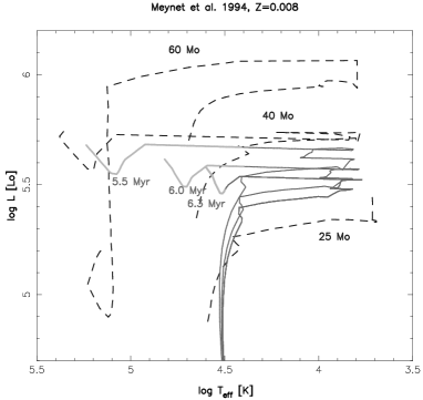
Figure 4: Evolutionary tracks (dashed line) and isochrones (solid lines) from Starburst99 and Meynet et al. (1994).

4.2 Minimum masses ${\cal M}^{min}[Q_{a_{\nu}}(X^{i})]$

Figure 5: ${\cal{M}}^{min}[Q_{a_{\nu}}(X^{i})]$ values as a function of time for different ions and metallicities using Starburst99 with stellar tracks with enhanced mass-loss rates, and atmosphere models by Smith et al. (2002). The values are normalised to 1 M_⊙ for a cluster with a Salpeter IMF in the mass range 0.1 – 120 M_⊙. Panel division and symbols like in Fig. 2.

Figure 6: Same as in Fig. 5, but using the CMHK code and standard mass-loss rate tracks. Panel division and symbols like in Fig. 2.

In analogy to our definition of the minimum mass associated to the LLL, we will define in the following a minimum mass associated to the effective rate of ionising photons, ${\cal M}^{min}[Q_{a_{\nu}}(X^{i})]$, which is defined as the mass of a stellar system with a completely sampled IMF and total effective rate of ionising photons equal to the maximum of all the effective rates provided by the individual stars in the system.

The evolution of ${\cal M}^{min}[Q_{a_{\nu}}(X^{i})]$ for the ions selected before, computed with Starburst99 and the CMHK code, are shown in Fig. 5 and 6 respectively. The organisation of the figures is the same as in Fig. 2. Perhaps the most striking feature of these results is the huge mass range covered, which spans nearly three orders of magnitude, from about $3\times 10^{3}$ to more than 10⁶ M_⊙ for some of the important ions, independently of the code used. As expected, the larger the ionising potential, the larger the minimum mass ${\cal{M}}^{min}[Q_{a_{\nu}}(X^{i})]$, since incomplete sampling affect mainly the most massive stars, which are those contribute most to this property. Likewise, S⁰ has the lowest ${\cal{M}}^{min}[Q_{a_{\nu}}(X^{i})]$ value: the ionising potential of S⁰ is only 10.36 eV, so the effective rate of ionising photons for this ion is scarcely affected by sampling effects. On the other hand, He⁺ is the ion more affected by sampling effects: this result confirms that He ii lines cannot be used as a strong constrain on the properties of stellar clusters, as suggested by Luridiana et al. (2003b).

The most prominent peak in ${\cal{M}}^{min}[Q_{a_{\nu}}(X^{i})]$ corresponds to the WR phase of the cluster. In the case of Starburst99, there is a tendency to obtain larger ${\cal{M}}^{min}[Q_{a_{\nu}}(X^{i})]$ values during the WR-phase at intermediate metallicities ($Z$=0.008), and an asymmetric “U-shaped” curve at low metallicities. We have tested this behaviour obtaining the corresponding ${\cal{M}}^{min}[Q_{a_{\nu}}(X^{i})]$ with the CMHK code using the evolutionary tracks by Meynet et al. (1994), and the “U-shaped” behaviour remains. However, ${\cal{M}}^{min}[Q_{a_{\nu}}(X^{i})]$ tends to be lower for larger metallicities. For the case of the CMHK code, the effect is explained easily: since the WR atmosphere models are the same for all the metallicities, the larger the metallicity, the larger the mass-loss rate, the lower the luminosity, and the lower ${\cal{M}}^{min}[Q_{a_{\nu}}(X^{i})]$. In the case of Starburst99 the effect of the metallicity-dependent WR atmosphere models must also be taken into account together with the variation of the luminosity with metallicity. In fact, examining the ionising fluxes quoted for the WR stars in tables 3 and 4 of Smith et al. (2002), it is found that the flux of ionising photons is not a monotonic function of the metallicity: the largest values for the rate of ionising photons correspond to some of the WR models at $Z$=0.008 ($Z$=0.4 $Z_{\odot}$ in their paper). This would be the origin of the larger ${\cal{M}}^{min}[Q_{a_{\nu}}(X^{i})]$ value at this metallicity. This also shows the impact of the use of metallicity-dependent atmosphere models for WR stars.

The “U-shaped” behaviour during the WR-phase is due to the evolutionary tracks used: since the lower the number of stars that dominate the luminosity, the larger the ${\cal{M}}^{min}[Q_{a_{\nu}}(X^{i})]$ value, its value depends on the relative rate of ionising photons emitted by WR stars with respect to the other hot stars in the synthetic cluster. In the tracks by Meynet et al. (1994), the WR stars at the beginning of the WR phase are also the most luminous stars in the cluster (see, for example, the 60 M_⊙ track in Fig. 4) with the harder ionising flux: this fact produces the first peak in ${\cal{M}}^{min}[Q_{a_{\nu}}(X^{i})]$. When the system evolves, the luminosity of WR stars decreases and the other non-WR, hot stars give only a small contribution (see, for example, the 40 M_⊙ track in Fig. 4), leading to the decrease in ${\cal{M}}^{min}[Q_{a_{\nu}}(X^{i})]$. However, since the non-WR stars become cooler as the age increases, at the end of the WR-phase WR stars become again the almost only source of ionising flux, producing the secondary peak. Note also that, for $Z$=0.040, the end of the WR-phase is marked by the highest peak in the curve: this behaviour is due to the longer duration of the WR-phase at this metallicity and to the dependency of the lifetime of massive stars with mass, which in these tracks is not monotonic: stars with initial mass of 85 and 120 M_⊙ stars end their evolution as WR at 5 and 8 Myrs respectively. As a consequence, in such an age range and at this metallicity, the ionising flux is dominated by the less populated tail of the IMF, so that sampling effects dominate and a larger ${\cal{M}}^{min}[Q_{a_{\nu}}(X^{i})]$ value is obtained.

The same general explanations also apply to the case of the CMHK results with standard mass-loss rate. However, for these tracks WR and non-WR stars have more similar luminosities and the first peak does not appear (the curve is “J-shaped”). In this case the maximum in ${\cal{M}}^{min}[Q_{a_{\nu}}(X^{i})]$ occurs at $Z$=0.004, because the WR phase is very short and almost absent at $Z$=0.001. In fact, at this metallicity, there no star ends its evolution as a WR; the WR-phase only appears in the middle of the 120 M_⊙ track, which ends as a supergiant.

There are also several peaks in ${\cal{M}}^{min}[Q_{a_{\nu}}(X^{i})]$ at the oldest ages considered in these plots. These features are an artefact of the way in which model atmospheres are assigned to stars in the synthetic HR diagram: since the smooth evolutionary path of each star in the HR diagram is coupled to a discrete ensemble of atmosphere models, a peak is produced when stars suddenly switch from one atmosphere model to the next. In the case of Starburst99, the effect is not too strong because this code uses a finer atmosphere grid. In the case of the CMHK code, the switch from the CoStar to the Kurucz (1991) atmosphere models for stars in the main sequence around $M=20$ M_⊙ produces the additional bumps in ${\cal{M}}^{min}[Q_{a_{\nu}}(X^{i})]$ with the most prominent ones ending at $t\approx$ 9.4 Myr for $Z$=0.001 and $Z$=0.004, $t\approx$ 9 Myr for $Z$=0.008, $t\approx$ 8.1 Myr for $Z$=0.020, and $t\approx$ 7 Myr for $Z$=0.040, corresponding to the turn-off age of a 20 M_⊙ star (point 13 in the tracks), the phase at which CoStar models are no longer used. Additional small bumps are found at the turn-off age of a 25 M_⊙. We want to remark again that these bumps are model artifacts, and that they would not appear if the atmosphere models were interpolated, instead of being computed by means of the “closest atmosphere model” approach.

Note that ${\cal M}^{min}[Q_{a_{\nu}}(X^{i})]$ corresponds to the amount of gas transformed into stars, and not to the total mass of the cluster (stars plus gas, that is dynamical mass, which would be approximately a factor of ten larger), and that a Salpeter IMF in the mass range 0.1 to 120 M_⊙ has been assumed. Table 1 gives conversion factors for different mass limits and also the numbers of stars for a Salpeter IMF. The results of Starburst99 are usually normalised to $10^{6}$ M_⊙ in the mass range 1–120 M_⊙, while CMHK normalise the results to 1 M_⊙ in the mass range 2–120 M_⊙.

	IMF mass range
Quantity	0.1-120	1-120	2-120	8-120	25-120	40-120
Mass into stars	1	0.3962	0.2912	0.1442	0.0668	0.0428
Number of stars	2.8290	0.1262	0.0494	0.0074	0.0014	0.0007

Table 1: Conversion factors for cluster masses and numbers of stars for different IMF mass ranges assuming a Salpeter slope.

Using the values in Table 1, a value of ${\cal{M}}^{min}[Q_{a_{\nu}}(X^{i})]$ around $3\times 10^{3}$ implies that there are, on average, two stars in the mass range 40–120 M_⊙, or 21 stars in the mass range 8–120 M_⊙. Since the most massive stars are also the most luminous ones, the ionisation of the cluster is accounted for by a few stars. The presence of a few WR stars, with a harder ionising flux, produces the increases in ${\cal{M}}^{min}[Q_{a_{\nu}}(X^{i})]$, especially for ions with higher energy edges. A straightforward conclusion follows from this result: the ionisation structure for clusters with ${\cal{M}}$ close to ${\cal{M}}^{min}[Q_{a_{\nu}}(X^{i})]$ would be better reproduced by the ionising spectrum of a single star rather than by the synthetic spectrum produced by a synthesis code, which always includes an ensemble of stars.

Figure 7: Relative dispersion $\sigma(Q_{a_{\nu}})/Q_{a_{\nu}}$ as a function of time for different metallicities and ions. Panel division and symbols like in Fig. 2.

It is necessary to recall, in this context, that ${\cal{M}}^{min}[Q_{a_{\nu}}(X^{i})]$ is, in fact, a rather restrictive lower limit for the use of integrated ionising spectra obtained by synthesis models. A better way to estimate when a composite spectrum begins to be a better approximation is given by the relative dispersion in $Q_{a_{\nu}}(X^{i})$ corresponding to ${\cal{M}}={\cal{M}}^{min}[Q_{a_{\nu}}(X^{i})]$, which is shown in Fig. 7. As expected, the dispersion varies strongly with the age, metallicity and ion under consideration, but, in general, it has a value around 60% (or, equivalently, ${\cal{N}}\sim 3$). This means that in order to obtain a dispersion smaller than 10% (${\cal{N}}=100$), clusters with initial masses ${\cal{M}}\mathrel{\hbox{\hbox to0.0pt{\hbox{\lower 4.0pt\hbox{$\sim$}}\hss}\hbox{$>$}}}33\times{\cal{M}}^{min}[Q_{a_{\nu}}(X^{i})]$ are needed. This is a good lower limit to ensure that the use of the composite ionising spectrum obtained from synthesis models is appropriate. For clusters with masses in the range [${\cal{M}}^{min}$, $33\times{\cal{M}}^{min}$] the situation is fuzzier, and any result obtained from codes which use a fully-sampled IMF must be taken with extreme caution. The only proper alternative solution in this case is to use Monte Carlo simulations.

4.3 Correlations between ionising bands

Figure 8: Linear correlation coefficient $\rho(X^{i},Y^{j})$ as a function of time for different metallicities and ions. The five main panels correspond to the metallicities $Z$=0.001 (top-left), $Z$=0.004 (top-right), $Z$=0.008 (middle), $Z$=0.020 (solar, bottom-left) and $Z$=0.040 (bottom-right). Each main panel is further subdivided into four sub-panels: the top-left sub-panel corresponds to $\rho(\mathrm{H}^{0},\mathrm{He}^{0})$, and $\rho(\mathrm{H}^{0},\mathrm{He}^{+})$; the top-right sub-panel corresponds to the correlation coefficients of ions with similar ionising potential; the bottom-left sub-panel corresponds to correlation coefficients related to the $\eta$ parameter; and the bottom-right sub-panel to correlation coefficients related to the [N ii] 6584/H$\alpha$ vs. [O iii] 5007/H$\beta$ diagram.

In this section, we will discuss the information that can be obtained through the study of the correlation coefficients $\rho[Q_{a_{\nu}}(X^{i}),Q_{a_{\nu}}(Y^{j})]$ between the effective rate of photons of the ions $X^{i}$ and $Y^{j}$. For the sake of simplicity, we will use in the following the notation $\rho(X^{i},Y^{j})\equiv\rho(Q_{a_{\nu}}(X^{i}),Q_{a_{\nu}}(Y^{j}))$.

As indicated in Section 2.2, a linear correlation coefficient $\rho(X^{i},Y^{j})$ close to unity indicates that $Q_{a_{\nu}}(X^{i})$ and $Q_{a_{\nu}}(Y^{j})$ are essentially produced by the same stars within a stellar population. Note that the correlation between observable quantities is not affected by sampling effects in the IMF; nevertheless, we take advantage of the statistical formalism introduced in Section 2.2 for the analysis of the effects of incomplete sampling to compute the values of the correlation coefficients.

The correlation coefficients between effective rates of ionising photons may provide useful insights into the concept of ionisation correction factors (icfs) used in abundance determinations. A correlation coefficient close to one is a necessary condition to relate the abundance of two different ions in a ionised nebula independently of the ionising stellar population. The assumption of the existence of general recipes relating the abundances of two ions is conceptually analogous to the one underlying the definition of the icfs. However, a correlation coefficient close to one is not a sufficient condition for a correct definition of the icfs, since the properties of the gas might also be relevant in the determination of the ionisation structure of a nebula (Luridiana et al. 2003a).

The correlation coefficients between the effective rates of ionising photons of different ions may also be used to make predictions on diagnostic diagrams. However, in the case of diagnostic diagrams an additional difficulty appears, because they do not relate absolute intensities but ratios. Hence, e.g., the correlation coefficients $\rho(\mathrm{H}^{0},\mathrm{N}^{0})$ and $\rho(\mathrm{H}^{0},\mathrm{O}^{+})$ are not sufficient to derive a correlation in the [N ii] 6584/H$\alpha$ vs. [O iii] 5007/H$\beta$ diagram, since it is also necessary to know $\rho(\mathrm{N}^{0},\mathrm{O}^{+})$. In addition, even in the case of a full linear correlation ($\rho=1$), the tilt of the regression line and the position of the mean value are required, so a photoionisation model is always needed. For the time being, we will only obtain the correlation coefficients, to see whether correlations exist. In Paper III we will apply these results to make predictions on the dispersion in the diagnostic diagram.

The results of the calculation of the correlation coefficients are shown in Fig. 8 for selected ions and diagnostic diagrams. It is interesting to compare this figure with Fig. 6, where ${\cal{M}}^{min}[Q_{a_{\nu}}(X^{i})]$ is given as a function of time for different metallicities and ions. A similar behaviour is observed in both figures: the larger the difference of the ${\cal{M}}^{min}[Q_{a_{\nu}}(X^{i})]$ values, the lower the correlation coefficient. This is easily understood: a larger difference in ${\cal{M}}^{min}$ means that the stars that contribute the most to the corresponding effective rates of ionising photons are different, and hence, the effective rates are loosely correlated.

In general, all correlation coefficients are close to unity until the WR phase begins. This phase introduces extra ionising photons associated with a handful of luminous stars, and hence destroy the correlations between the effective rates of ionising photons. Correlation coefficients closer to one are preferentially found at low metallicities, due to the paucity of WR stars.

Fig. 8 is divided into five main panels corresponding to different metallicities. Each main panel is further subdivided into four sub-panels: the top-left sub-panel shows $\rho(\mathrm{H}^{0},\mathrm{He}^{0})$, and $\rho(\mathrm{H}^{0},\mathrm{He}^{+})$, the top-right sub-panel shows the correlation coefficients of ions with similar ionising potential, the bottom-left sub-panel shows the correlation coefficients related to the $\eta$ parameter, and the bottom-right sub-panel the correlation coefficients related to the [N ii] 6584/H$\alpha$ vs. [O iii] 5007/H$\beta$ diagram.

The $\rho(\mathrm{H}^{0},\mathrm{He}^{0})$ and $\rho(\mathrm{H}^{0},\mathrm{He}^{+})$ correlation coefficients have values significatively different from 1 starting from the onset of the WR-phase. The larger the metallicity, the lower the correlation coefficient, implying that the ratios $Q(\mathrm{He}^{0})/Q(\mathrm{H}^{0})$ and $Q(\mathrm{He}^{+})/Q(\mathrm{H}^{0})$ are not robust constraints of the general properties of a cluster (like the upper mass limit in the IMF, the IMF slope, and the age): they are quite dependent on the particular stellar populations in the cluster and their value can strongly vary from cluster to cluster, especially for poorly populated high metallicity regions (see, for example, Bresolin & Kennicutt 2002). On the other hand, for the same reason they can be used to infer the relative abundance of particular populations in a given observed cluster.

The correlation coefficients shown in the top-right sub-panels are $\rho(\mathrm{H}^{0},\mathrm{O}^{0})$ (the two ions having ionising potentials of 13.599 and 13.618 eV respectively), $\rho(\mathrm{He}^{0},\mathrm{S}^{+})$ (ionising potentials of 24.588 and 23.330 eV respectively), $\rho(\mathrm{He}^{+},\mathrm{O}^{++})$ (ionising potentials of 54.418 and 54.936 eV respectively), and $\rho(\mathrm{O}^{+},\mathrm{S}^{++})$ (ionising potentials of 35.118 and 34.830 respectively). With the only exception of $\rho(\mathrm{He}^{+},\mathrm{O}^{++})$, the correlation coefficients are pretty close to 1 in all the cases, as expected during the WR phase. In contrast, the correlation coefficient of $\rho(\mathrm{He}^{+},\mathrm{O}^{++})$ does not have a constant value, but surprisingly varies between values close to one and values close to zero. The zero value does not necessarily imply that the two quantities are not correlated in the corresponding age ranges: it rather indicates that one or both of the $Q_{a_{\nu}}$ values are zero, that is $\rho(\mathrm{He}^{+},\mathrm{O}^{++})=0$ implies the absence of photons above 54.418 eV in the model atmospheres of stars at the corresponding ages.

The bottom-left sub-panels correspond to correlation coefficients related to the $\eta$ parameter, that is the ratio of $\mathrm{O}^{+}/\mathrm{O}^{++}$ to $\mathrm{S}^{+}/\mathrm{S}^{++}$ (Vílchez & Pagel 1988). Note that the $\eta$ parameter is measured from forbidden lines, thus it is related to $Q_{a_{\nu}}(\mathrm{O}^{0})$, $Q_{a_{\nu}}(\mathrm{O}^{+})$, $Q_{a_{\nu}}(\mathrm{S}^{0})$ and $Q_{a_{\nu}}(\mathrm{S}^{+})$. In general, the correlation coefficients involving $\mathrm{S}^{0}$ are markedly lower than 1. Remember that $\mathrm{S}^{0}$ was the ion with the lowest ${\cal{M}}^{min}$, which also means that it is produced by a population of stars different from those responsible for the ionising flux (in fact, it is produced by the ionising stars plus other stars): this fact naturally produces a poor correlation. As in the case of $\rho(\mathrm{H}^{0},\mathrm{He}^{0})$ and $\rho(\mathrm{H}^{0},\mathrm{He}^{+})$, the $\eta$ parameter is not a good parameter to constrain the age of the cluster, but it is a good parameter to determine the relative proportion of non-ionising and ionising stars, and the softness of the ionising radiation for specific clusters.

Finally, the interesting correlation coefficients $\rho(\mathrm{H}^{0},\mathrm{O}^{+})$ and $\rho(\mathrm{N}^{0},\mathrm{O}^{+})$, together with $\rho(\mathrm{H}^{0},\mathrm{N}^{0})$, can be used to estimate the dispersion in the [N ii] 6584/H$\alpha$ vs. [O iii] 5007/H$\beta$ diagram. The effective rates of ionising photons $Q_{a_{\nu}}(\mathrm{H}^{0})$ and $Q_{a_{\nu}}(\mathrm{N}^{0})$ are strongly correlated, implying that the abundances of the two ions are linearly dependent. In turn, this relation suggests that both elements will show a similar correlation with O⁺, a fact confirmed by $\rho(\mathrm{H}^{0},\mathrm{O}^{+})$ presenting a behaviour similar to $\rho(\mathrm{N}^{0},\mathrm{O}^{+})$. This has an additional implication: the position of data points in the [N ii] 6584/H$\alpha$ vs. [O iii] 5007/H$\beta$ diagram depends on two variables only (either O⁺ and H⁰ or O⁺ and N⁰), and so the data points will lie on a uniparametric line rather than being spread on the entire plane. Hence, the correlation coefficients obtained through the analysis of the sampling effects may explain the fact that observational data follow a narrow sequence. However, the sequence is uniparametric only for a given metallicity, and it could be different when metallicity varies, yielding a larger scatter in the diagnostic diagram. That is, in fact, the situation in the lower region of this diagram, which is populated by data points corresponding to different metallicities.

5 Conclusions

In this paper we have presented an evaluation of the dispersion in the properties of the ionising flux obtained from synthesis models due to the IMF sampling. The ionising fluxes have been characterised by appropriate physical quantities, the effective rates of ionising photons, which are obtained from the integration of the ionising flux weighed by the photoionisation cross section of different ions, with the future goal of using them in the evaluation of sampling effects on emission line spectra.

We have obtained the effective rate of ionising photons for a wide set of metallicities and atmosphere models, comparing the results of two different codes to assess some of the systematic effects. The analysis of the effective rates obtained with different model atmospheres is consistent with previous studies on the impact of the atmosphere models on the ionising flux of star forming regions, and it additionally provides a proper statistical ground for such assessments. We have identified problems in the computation of the ionising flux in regimes where stellar evolution does not present a continuous behaviour with the initial stellar mass, such as at the end of the WR phase.

We have computed the corresponding minimum initial cluster masses for which the ionising continuum obtained by synthesis models can be applied. The minimum masses range from 10³ to more than 10⁶ M_⊙ depending on the metallicity and the age of the stellar population. For observed clusters with stellar masses below the minimum mass, the ionising flux is better accounted for by a single star, rather than by a population of massive stars, so that the use of synthesis models is not appropriate in these cases. We have also evaluated the dispersion in the distribution of the effective rates of ionising photons at the minimum mass, and found it to be around 60%. This means that the initial mass of observed stellar clusters must be larger than a minimum value in the range $3\times 10^{4}$ M_⊙ to $3\times 10^{7}$ M_⊙, depending on age and metallicity, in order for evolutionary synthesis models that assume a completely sampled IMF to be applied. We have also found indications suggesting that the emission of [S ii] is much less affected by sampling effects than that of other ions. The He ii lines are in turn the most affected by sampling, especially during the WR phase, and should not be used to constrain the evolutionary status of stellar clusters.

We also studied the correlations between different effective rates of ionising photons, finding in some cases correlation coefficients close to one. This result agrees with the observational finding that H ii regions over a vast range of scales, ranging from those ionised by single stars to those ionised by super-stellar clusters, are found in a relatively narrow band in some emission-line diagnostic diagrams.

Tables containing the effective rate of ionising photons, their corresponding $\cal{N}$, the corresponding LLL, and the complete correlation matrix for H⁰, He⁰, He⁺, N⁰, N⁺, N⁺⁺, O⁰, O⁺, O⁺⁺, S⁰, S⁺, S⁺⁺, C⁰, Ne⁰, Ne⁺, Ar⁰, Ar⁺, and Ar⁺⁺ ions are available at the www address http://laeff.inta.es/users/mcs/SED/. They include the results using the CMHK code with standard and high mass-loss rate.