Physical limits to the validity of synthesis models

In this paper we establish a necessary condition for the application of stellar population synthesis models to observed star clusters. Such a condition is expressed by the requirement that the total luminosity of the cluster modeled be larger than the contribution of the most luminous star included in the assumed isochrones, which is referred to as the Lowest Luminosity Limit (LLL). This limit is independent of the assumptions on the IMF and almost independent of the star formation history. We have obtained the Lowest Luminosity Limit for a wide range of ages (5 Myr to 20 Gyr) and metallicities ($Z$=0 to $Z$=0.019) from the Girardi et al. (2002) isochrones. Using the results of evolutionary synthesis models, we have also obtained the minimal cluster mass associated with the LLL, ${\cal M}^{min}$, which is the mass value below which the observed colors are severely biased with respect to the predictions of synthesis models. We explore the relationship between ${\cal M}^{min}$ and the statistical properties of clusters, showing that the magnitudes of clusters with mass equal to ${\cal M}^{min}$ have a relative dispersion of 32% at least (i.e., 0.35 mag) in all the photometric bands considered; analogously, the magnitudes of clusters with mass larger than $10\times{\cal M}^{min}$ have a relative dispersion of 10% at least. The dispersion is comparatively larger in the near infrared bands: in particular, ${\cal M}^{min}$ takes values between 10⁴ and 10⁵ M_⊙ for the $K$ band, implying that severe sampling effects may affect the infrared emission of many observed stellar clusters. As an example of an application to observations, we show that in surveys that reach the Lowest Luminosity Limit the color distributions will be skewed toward the color with the smallest number of effective sources, which is usually the red, and that the skewness is a signature of the cluster mass distribution in the survey. We also apply our results to a sample of Globular Clusters, showing that they seem to be affected by sampling effects, a circumstance that could explain, at least partially, the bias of the observed colors with respect to the predictions of synthesis models. Finally, we extensively discuss the advantages and the drawbacks of our method: it is, on the one hand, a very simple criterion for the detection of severe sampling problems that bypasses the need for sophisticated statistical tools; on the other hand, it is not very sensitive, and it does not identify all the objects in which sampling effects are important and a statistical analysis is required. As such, it defines a condition necessary but not sufficient for the application of synthesis models to observed clusters.

1 Introduction and motivation

The comparison between theoretical models and observations is the basic procedure that allows the evaluation of our current knowledge of Nature; underlying this statement is the assumption that better observational data, by setting more stringent constraints, make such comparison more meaningful. Although this is almost always the case, there is a situation in which, paradoxically, the opposite is true, and the more the data quality improves, the more biased the theoretical inferences turn out to be. This is indeed the case of the analysis of the integrated light of stellar populations. The progressively higher sensitivity of modern instruments provides access to data from increasingly fainter stellar clusters, up to a point where we must begin to take into account the limitations posed by the discreteness of the number of stars in a system: due to incomplete sampling, both small clusters and small samples of large clusters have stellar mass distributions that may differ substantially from the one predicted by the underlying initial mass function (IMF). Nevertheless, most theoretical models assume that the IMF of clusters is completely populated, i.e., that the distribution of stellar masses is continuous and that all the evolutionary stages are well sampled. Obviously, any model assuming a continuous IMF (hereinafter, analytical models) will be correct only under the asymptotic assumption of an infinite number of stars. Hence, the validity of the comparison between the predictions of synthesis models and real systems, where the IMF is not perfectly sampled, depends on the size of the system.

Several works have been written that deal directly or indirectly with the subject of sampling effects. For example, Barbaro & Bertelli (1977), Chiosi et al. (1988), Girardi & Bica (1993), and Girardi et al. (1995), who show the relevance of sampling effects for the study of LMC clusters; Santos & Frogel (1997), who determine how sampling effects affect integrated near-infrared colors; Cerviño, Luridiana, & Castander (2000) and Cerviño et al. (2000), who study the effects of sampling in some observables of young star-forming regions; Cerviño et al. (2001a) and Cerviño & Mollá (2002), who estimate the effects of sampling in stellar yields and chemical evolutionary models. Sampling effects also underlie the study of surface brightness fluctuations (Tonry & Schneider 1988), a primary distance indicator that is based on the analysis of the variations with distance of the amount of stars sampled by CCD pixels: for example, Cantiello et al. (2003) show that surface brightness fluctuations may suffer from a bias that depends on the density of stars in the image pixels.

In almost all the preceding works, sampling effects have been evaluated by the use of Monte Carlo simulations. Alternatively, Cerviño et al. (2002b) proposed a formalism, based on the original formulation by Buzzoni (1989), where the mean value, the dispersion, and the correlation coefficient of different observables are obtained analytically using a continuously distributed IMF. The method is applied to young star-forming regions ($t<20$ Myr) and compared with the results of Monte Carlo simulations, showing that in both cases the results are quite similar, except for colors and equivalent widths in clusters with a low number of stars. The method is extensively tested in Cerviño & Valls-Gabaud (2003) for clusters with a number of stars between 1 and 10³, where it is shown that it reproduces the average value and the dispersion of quantities obtained from Monte Carlo simulations, i.e., the luminosities of Monte Carlo simulations are distributed around the mean value obtained from the analytical model, if the quantity scales linearly with the amount of stars in the system. However, when the modeled properties are logarithmic quantities or ratios, as in the case of equivalent widths and colors, the mean values of Monte Carlo simulations are biased with respect to the results of the analytical modeling; the smaller the system, the more severe the bias. Unfortunately the authors are not able to quantify this bias in an analytical way for very small systems.

The subject of sampling has also been addressed by, e.g., Lançon & Mouhcine (2000), Girardi (2000), Cerviño et al. (2001b), Bruzual (2002), Girardi (2002), Cerviño et al. (2002a), Cerviño & Luridiana (2002a, b), Cerviño & Valls-Gabaud (2002), and Cerviño (2003a, b, c, d). However, since all these works are published in conference proceedings, their consequences are not extensively explored. Lançon & Mouhcine (2000) evaluate sampling effects on monochromatic luminosities at solar metallicity without the use of Monte Carlo simulations, and quote some limits for the minimal initial clusters masses ensuring a relative error lower than 10% for some ages and luminosities. Bruzual (2002) (see also Bruzual & Charlot 2003) presents Monte Carlo simulations in which the stochastic effects on $U-B$, $B-V$, $V-K$, and $K$ for the LMC metallicity are presented as a function of the initial mass of the cluster. His figures show clearly that there is a bias in the results of Monte Carlo simulations with respect to the results of analytical synthesis models; however, this result is not mentioned in the text, possibly due to the limited space. Finally, Girardi (2002) presents Monte Carlo simulations where the effect of a continuous distribution in the initial cluster masses is studied. His results are more appropriate for the comparison with surveys of real clusters than those that do not consider a distribution of masses.

In all the preceding papers, the evaluation of sampling effects requires making assumptions on the IMF and the star formation history, a fact that limits the practical application of the results to real observations. In this paper we propose instead a method entirely based on observable quantities, therefore independent of the IMF and almost independent of the star formation history, to estimate whether the colors predicted by synthesis models are biased with respect to real observations, and to establish when analytical synthesis models cannot be applied and a statistical formulation is required. We also describe the relationship of this method to more sophisticated statistical analyses. Furthermore, we suggest examples of possible applications of the method to the analysis of observational data. Finally, we discuss the qualities and drawbacks of our method in comparison to alternative ones.

The structure of the paper is the following: in Sect. 2 we define the method, and provide a quantitative evaluation of the quantities involved for a wide range of observational cases; in Sect. 3 we translate the preceding results in terms of the cluster masses, proposing a mass criterion to exclude low-statistics clusters from the analysis performed with synthesis models; in Sect. 4 we show the observational implications of this work; in Sect. 5 we discuss the limitations of our results; and in Sect. 6 we draw our conclusions.

2 The Lowest Luminosity Limit

One of the most basic limits to the application of evolutionary synthesis models can be expressed by the following statement:

The total luminosity of the cluster modeled must be larger than the individual contribution of any of the stars included in the model

This obvious statement defines a natural theoretical limit that has not always been considered when models are applied to real observations. Whereas in the work by Tinsley (see, e.g., Tinsley & Gunn 1976) it was not necessary to take this limit into account, due to the observational limitations at that epoch, the increasing sensitivity of current instruments has reached a level where this limitation plays a fundamental role in the interpretation of data.

Defining as the Lowest Luminosity Limit (hereinafter LLL) the luminosity of the brightest individual star included in the model, we can establish a simple luminosity criterion for the application of synthesis models to the interpretation of observed clusters, imposing the condition that the cluster modeled be more luminous than the LLL. While clusters brighter than this limit may either be well-sampled or not, clusters fainter than this limit are certainly misrepresented by synthesis models.

It is possible to establish a luminosity limit following different criteria, yielding either weaker or more stringent constraints; but all the alternative definitions we could think of turned out to either lack physical meaning, or imply circumstances that do not occur in the modeling practice. Nevertheless, the degree of arbitrariness of our definition is a hairy problem, and we will discuss it thoroughly in Sect. 5.

With the definition given above, the LLL is only defined by the isochrone used and the band under consideration; however, its exact value at a given age is also weakly dependent on the star formation history. In the following we present the values of the LLL computed for a wide range of parameters. We have used the isochrones and the integrated magnitudes of simple stellar population models (hereinafter SSP models, i.e., models that assume an instantaneous burst of star formation) by Girardi et al. (2002). We consider seven different metallicities: $Z$=0.019 (solar), $Z$=0.008, $Z$=0.004, $Z$=0.001, $Z$=0.0004, $Z$=0.0001, and $Z$=0.0. The $Z$=0.0 isochrones correspond to metal-free models by Marigo et al. (2001). The other isochrones correspond to the basic set presented in the web server cited in the footnote, which combines the results from Girardi et al. (2000) and Girardi (2001) for low- and intermediate-mass stars, with the results by Bertelli et al. (1994) and Girardi et al. (1996) for high-mass stars, and that includes overshooting and a simplified Thermal Pulse AGB (TP-AGB) evolution. Additionally, for $Z$=0.019, 0.008, and 0.004 we have used the isochrones by Marigo & Girardi (2001) that include a more detailed TP-AGB evolution. Most of the atmosphere models are taken from ATLAS9 (Castelli et al. 1997). A more detailed description of the isochrones, the atmosphere models, and the SSP models can be found in Girardi et al. (2002) and in their web server.

To obtain the LLL we have searched for the bolometric luminosity of the most luminous star in any given isochrone $L^{max}_{bol}(t)$. However, since the tabulated data also provide the magnitudes at different bands, we have also obtained the magnitude of the most luminous star in the Johnson-Cousins-Glass filters $U$, $B$, $V$, $R$, $I$, $J$, $H$, and $K$: $M^{min}_{U}(t)$, …, $M^{min}_{K}(t)$.

In general, the most luminous star is also the most evolved, but this relation does not strictly hold for all the bands nor all the ages. This fact is well illustrated in Fig. 1, where the LLLs obtained from isochrones with a simplified TP-AGB treatment (right panels) are compared with the LLL obtained from isochrones with a detailed TP-AGB evolution (left panels) for models with $Z$=0.019, 0.008, and 0.004. Whereas $M^{min}_{U,B,V,R,I}$ depend on the TP-AGB treatment at some ages, $M^{min}_{bol,J,H,K}$ are almost unaffected by it.

Figure 1: LLL in magnitudes for the bolometric luminosity and different bands, as a function of the age for three different metallicities: top panels $Z$=0.019 (solar); middle panels $Z$=0.008; and bottom panels $Z$=0.004. Left panels correspond to isochrones with a simplified TP-AGB evolution, and right panels to isochrones with a detailed TP-AGB evolution. The different lines correspond to the following: bold solid line: bolometric magnitude; solid line with triangles: $U$; dashed line: $B$; dot-dashed line with triangles: $V$; dotted line: $R$; dash-dot-dot-dotted line: $I$; solid line: $J$; dashed line with triangles: $H$; and dot-dashed line: $K$.

Figure 2: LLL in magnitudes for the bolometric luminosity and different bands, as a function of the age for $Z$=0.001 (top left), $Z$=0.0004 (top right), $Z$=0.0001 (middle left) and $Z$=0 (middle right). Symbols like in Fig. 1. The bottom panel compares the LLL for $V$ and $K$ for $Z$=0.019 and $Z$=0.0001.

Figures 1 and 2 show the values of the LLL in magnitudes for different ages and metallicities. The figures show that $M^{min}(t)$ evolves with time toward less luminous values for all the bands, and that blue bands become fainter more quickly than red bands, as expected due to the cluster evolution: the population becomes redder and fainter as the cluster evolves. These two trends combined imply that, as the cluster ages, the LLL tend to decrease (i.e., become less stringent) in all bands, doing so more rapidly at blue wavelengths than at red wavelengths. It is also interesting to compare the evolution of $M^{min}_{bol}(t)$ with the various $M^{min}(t)$ at different bands. It can be seen that the larger the metallicity, the more similar is the evolution of $M^{min}_{bol}(t)$ to the evolution of $M^{min}(t)$ in red bands, as a consequence of the increasing fraction of bolometric light that goes into red filters. The bottom panel in Fig. 2 compares the LLL values for $V$ and $K$ and two extreme metallicities. It can be seen that $M^{min}_{K}$ is almost metallicity-independent.

These figures show the LLL values for the case of single isochrones, that correspond to SSP models. However, the LLL can be easily obtained for different star formation histories. For example, let us consider a two-burst system with ages $t_{1}$ and $t_{2}$, associated to two minimum magnitude values $M^{min}(t_{1})$ and $M^{min}(t_{2})$: then the LLL of this system is simply the minimum of $M^{min}(t_{1})$ and $M^{min}(t_{2})$. In the case of a cluster with constant star formation history and age $t$, the LLL at each band is given by the maximum of the luminosity of SSP models in the age range between $0$ and $t$, which, for the bolometric luminosity, can be roughly approximated by the ZAMS luminosity of the most massive star included (this result is not exact because the bolometric luminosity of a star briefly increases after the ZAMS). At other bands the maximum luminosity can be reached much later, thus no easy recipe can be given. As a final remark, note that some evolution in the metallicity is expected for any star formation history different from an instantaneous burst, and this effect should be included in the modeling in a self-consistent way (see Schulz et al. 2002, and references therein as an example).

Summarizing, the most luminous star in one band is not necessarily the most luminous star in the rest of the bands, neither is it the star with the largest bolometric luminosity. As a consequence, the LLL depends not only on the age and the metallicity (i.e., the assumed isochrones and atmosphere libraries), but also on the band considered. The dependence on age and metallicity is weaker for the near infrared bands than for the optical bands. In particular, the LLL for $K$ is almost metallicity-independent.

3 Minimal initial cluster masses

In this section we will translate the concept of LLL into an equivalent formulation in terms of mass.

Let us recall that evolutionary synthesis models are based on the convolution of isochrones with the IMF and the star formation history. For the case of a SSP, the mean luminosity in a given band and at a given age, $l^{ssp}(t)$, results from the sum of the luminosities of individual stars at the corresponding age as given by the isochrone, $l_{i}(m_{i},t)$, weighted by the number of stars with initial mass $m_{i}$ as given by the IMF, $w_{i}(m_{i})$. If the sum of the $w_{i}$ values is normalized, as usual, to 1 M_⊙ transformed into stars from the onset of the burst, the resulting luminosity will also be normalized. The total luminosity of a modeled cluster, $L^{clus}(t)$, is directly proportional to the initial mass transformed into stars in the cluster, $\cal M$:

$$L^{clus}(t)={\cal M}\times{\sum w_{i}(m_{i})\,l_{i}(m_{i},t)}={\cal M}\times l^{ssp}(t).$$ (1)

Then, for a given age and metallicity, we can obtain the total initial mass transformed into stars from the observed luminosity $L^{clus}$ (or $M^{clus}$ expressed in magnitudes) and the corresponding normalized value of $l^{ssp}(t)$ (or $m^{ssp}$):

$${\cal M} = \frac{L^{clus}}{l^{ssp}},$$

$$2.5\log{\cal M} = m^{ssp}-M^{clus},$$ (2)

where we have dropped the explicit reference to $t$ to simplify the notation. Now, imposing that $M^{clus}=M^{min}(t)$, we can obtain the initial cluster mass for each band and age, ${\cal M}^{min}(t)$, for which the total luminosity of the cluster simulated by a SSP model equals the luminosity of the most luminous star in the band, $M^{min}(t)$:

$$2.5\log{\cal M}^{min}(t)=m^{ssp}(t)-M^{min}(t).$$ (3)

The superindex min reminds that below this limit the cluster cannot be modeled by means of a synthesis model. Note that ${\cal M}^{min}(t)$ depends on the age and the band, but also on the IMF and the star formation history, since integrated quantities depend on them. Here, we have used the integrated magnitudes of the SSP models by Girardi et al. (2002), which assume the IMF by Kroupa (2001) in its corrected version (his Eq. 6), and a total SSP initial mass equal to 1 M_⊙ in the mass range 0.01 – 120 M_⊙.

Figure 3: ${\cal M}^{min}$ for the bolometric luminosity and different bands, as a function of the age and the metallicity. Symbols as in Fig. 1.

The results for different ages and metallicities are shown in Fig. 3, which shows that ${\cal M}^{min}_{bol,J,H,K}$ are almost metallicity independent except during the first stages of the evolution of the cluster. In the case of optical bands, the lower the metallicity, the larger ${\cal M}^{min}_{U,B,V,R,I}$. The value of ${\cal M}^{min}$ spans three orders of magnitude depending on the band, and it takes a value as large as 10⁴ M_⊙ or even more for the case of near infrared colors. A first conclusion we can draw from these figures is that these values are so high that many observed clusters certainly fall below this limit, and their properties can by no means be reproduced by synthesis models. This fact is too often overlooked, and we will try to emphasize it repeatedly throughout the paper.

In order to examine the influence of the IMF on this result, we have also obtained the LLL from the isochrones by Girardi et al. (2000), which have been computed assuming a Salpeter IMF (Salpeter 1955) in the mass range 0.039 to 100 M_⊙ from 63 Myr to 17.8 Gyr. For a comparison with Girardi et al. (2002) we have renormalized these values to the mass range 0.094 – 120 M_⊙ in such a way that the fraction of mass in the range 1 – 120 M_⊙ for the Kroupa’s and the Salpeter’s IMF is the same. The comparison between the ${\cal M}^{min}$ values obtained from the two sets of isochrones and SSP models is shown in Fig. 4. With this normalization, the ${\cal M}^{min}$ values obtained using the models by Girardi et al. (2000) coincide for $V$ with those obtained using the models by Girardi et al. (2002) at ages smaller than 80 Myr, and for $K$ in all the age range in common. The differences in $V$ for $t>80$ Myr are due to small differences in the LLLs computed with the different set of isochrones.

Figure 4: ${\cal M}^{min}$ for $V$ (solid line with triangles) and $K$ (dashed line with diamonds) assuming solar metallicity and different IMF and SSP models: SSP models by Girardi et al. (2002) with the IMF by Kroupa (2001) (G02: bold line), and SSP models by Girardi et al. (2000) with Salpeter’s IMF (G00: narrow line). The figure also shows the minimal clusters masses that ensure $\sigma_{L}/L=10$% from Cerviño et al. (2002b) models (C02: big open symbols until age of 10 Myr), Worthey (1994) models (W94: big open symbols with ages larger than 1 Gyr) and Lançon & Mouhcine (2000) models (LM00: small open symbols).

3.1 Minimal initial cluster mass and the estimation of sampling effects (theoretical point of view)

Neither the computation of LLL nor that of ${\cal M}^{min}$ allow, by themselves, an evaluation of the extent of sampling effects in observed clusters: they just provide an easy-to-use cutoff criterion to discriminate clusters with severe sampling effects from clusters with more moderate or negligible sampling effects, without providing a quantitative tool to estimate their statistical properties.

In spite of this limitation, ${\cal M}^{min}$ is intrinsically related to sampling effects, and it is worth studying the relation between the information provided by ${\cal M}^{min}$ and the statistical properties of clusters. In such a way, it will be possible to obtain hints on the necessity to account for sampling effects in the interpretation of observed data, even without a proper statistical formalism.

To study the relation between the ${\cal M}^{min}$ value and the sampling effects, we have derived the values of the cluster masses associated to a relative dispersion of 10% in the luminosity of a band, ${\cal M}_{10\%}$; note that a relative dispersion of 10% in the luminosity means, at zero order approximation, $\sigma=0.1$ mag in magnitude.

To cover a wide age range, we have used the results of three different synthesis codes. For young ages, we have used the solar metallicity results from Cerviño et al. (2002b) models. These models have been computed using the Geneva evolutionary tracks with a Salpeter IMF in the mass range 2 – 120 M_⊙. In these models, sampling effects are evaluated by means of an effective number of stars that contribute to a given observable, ${\cal N}^{ssp}$, which is defined by:

$$\frac{1}{{\cal N}^{ssp}}=\frac{\sigma^{2}({l^{ssp}})}{(l^{ssp})^{2}}=\frac{\sum w_{i}\,l^{2}_{i}}{(\sum w_{i}\,l_{i})^{2}},$$ (4)

as first derived by Buzzoni (1989). Since the tabulated ${\cal N}^{ssp}$ values are normalized to ${\cal M}$, the value of ${\cal M}_{10\%}$ is trivially obtained imposing that $\sigma_{L}/L=0.1$; therefore, the absolute effective number of stars associated to ${\cal M}_{10\%}$ is ${\cal N}={\cal N}^{ssp}\times{\cal M}_{10\%}=100$.

For intermediate ages, we have used the results quoted by Lançon & Mouhcine (2000) that assume solar metallicity and a Salpeter IMF in the mass range 0.1 – 120 M_⊙. The models have been computed with the population synthesis code pegase (Fioc & Rocca-Volmerange 1997).

For old stellar populations ($t>1.5$ Gyr) we have used the solar metallicity SSP models by Worthey (1994) computed for a Salpeter IMF in the mass range 0.1 – 2 M_⊙ and normalized to ${\cal M}=10^{6}$ M_⊙. This author does not compute directly sampling effects, but they can be inferred from the fluctuation luminosities, $\bar{l}^{ssp}$. These $\bar{l}^{ssp}$ (or $\bar{m}^{ssp}$ expressed in magnitudes) are defined as:

$$\bar{l}^{ssp}=\frac{\sum w_{i}\,l^{2}_{i}}{\sum w_{i}\,l_{i}},$$ (5)

and they are computed for the evaluation of surface brightness fluctuations. From Eqs. 4 and 5 it is found that ${\cal N}^{ssp}\times\bar{l}^{ssp}=l^{ssp}$ (see Buzzoni 1993, for a general description of the relation between ${\cal N}^{ssp}$ and the brightness fluctuations). The corresponding ${\cal N}^{ssp}$ can be obtained as a function of $\bar{l}^{ssp}$ and $l^{ssp}$ (or $\bar{m}^{ssp}$ and $m^{ssp}$ in magnitudes) using the following formulae:

$${\cal N}^{ssp}\times 10^{6} = \frac{l^{ssp}}{\bar{l}^{ssp}},$$

$$2.5\log{\cal N}+15 = \bar{m}^{ssp}-m^{ssp},$$ (6)

where the factor $10^{6}$ (or $15=2.5\log 10^{6}$ in magnitudes), is used to renormalize his tabulated data to ${\cal M}=1$ M_⊙ following a Salpeter IMF slope in the mass range 0.1 – 2 M_⊙.

Note that Lançon & Mouhcine (2000) and Cerviño et al. (2002b) quote the dispersion for the monochromatic luminosities at the effective wavelength of the band (see King 1952, for the definition of effective wavelength) whereas Worthey (1994) (Eq. 6) gives the dispersion of the integrated luminosity of the band. In spite of this difference, these results can be directly compared: in fact, wide-band luminosities can be estimated, with an accuracy of 2 – 3%, by multiplying the monochromatic luminosities at the effective wavelength by a constant value, which represents the absolute flux density in the band (King 1952; Johnson 1966); since this transformation only implies the multiplication by a constant, which cancels out in the computation of the variance, the relative dispersion of the monochromatic luminosity is equal to the relative dispersion of the luminosities in the band obtained from the exact integration of the spectrum over the filter response. Therefore, the results by Lançon & Mouhcine (2000) and Cerviño et al. (2002b) and those by Worthey (1994) quoted above can be directly compared.

In all the cases we have renormalized the resulting values to a Salpeter IMF in the mass range 0.094 – 120 M_⊙. The results are shown with open symbols in Fig. 4. A first comparison among the ${\cal M}_{10\%}$ results show that they are quite consistent with each other, with some differences that can be attributed to the difference between the ${\cal N}$ formalism and the method applied by Lançon & Mouhcine (2000). The figure also shows that the evolution of ${\cal M}^{min}$ is quite similar to the evolution of ${\cal M}_{10\%}$. The differences in the two curves range between 0.98 and 1.5 dex (i.e., factors between 8 and 30 in initial cluster masses) depending on the age and the band. Therefore, for the assumed IMF and rounding up numbers, we can say that ${\cal M}^{min}$ is always at least a factor 10 below ${\cal M}_{10\%}$; this implies an ${\cal N}$ value lower than 10 and relative dispersions larger than 32% ($\sigma>0.35$ mag). For these values of ${\cal N}$, Poisson statistics produce non negligible probabilities of zero effective sources, and hence the presence of biases in colors, as shown in Cerviño & Valls-Gabaud (2003).

The relation between ${\cal N}$ and the occurrence of dispersion and of a bias can be easily understood in the following terms. Let us take as an example the case of $V-K$, and assume that $L^{LLL}_{K}$ corresponds to the luminosity of a star in the Red Supergiant (RSG) phase. Let us also assume the case of a 10 Myr old burst with solar metallicity, where, according to analytical models, more than 90% of the luminosity in $K$ is due to RSGs. For this case, comparing the corresponding ${\cal N}^{ssp}(L_{K})$ value with the (normalized) number of RSGs, $n^{ssp}_{RSG}$, it is found that $n^{ssp}_{RSG}\sim 0.9\times{\cal N}^{ssp}(L_{K})$ (see Cerviño et al. 2002b, and the web server mentioned above). For simplicity we will assume that ${\cal N}(L_{K})=N_{RSG}$, the absolute number of RSGs. Finally let us assume that ${\cal N}$ follows Poisson statistics, or, in terms of RSGs, that the number of such stars in different clusters is distributed following a Poisson distribution with a mean value $N_{RSG}$.

Since the contribution of RSG stars has a small influence on $V$ and a large influence on $K$, clusters in a mass range in which variations of $\pm 1$ in the number of such stars are relevant will have colors considerably redder (dominated by an excess of RSGs) or bluer (due to a deficit of RSGs) than those predicted by analytical synthesis models. Furthermore, if the mass of the cluster is such that $1<{\cal N}<10$, according to Poisson statistics there is a fair probability that the cluster has no RSGs at all. In this last case $(V-K)^{clus}$ will be more similar to the colors of main sequence (MS) stars than to the colors of SSP models (i.e., there will be an excess of blue clusters in a survey of clusters with this mass, age, and metallicity). For these values of ${\cal N}$ the dispersion in the colors will be the largest. Finally, if ${\cal N}$ takes values lower than 1, there will be an important fraction (or, in extreme cases, even a majority) of clusters without RSG stars, and then, the mean value of the observed color $(V-K)^{clus}$ will be biased with respect to the resulting color $(V-K)^{ssp}$ of a synthesis model. On the other hand, the dispersion will decrease since the range of possible $(V-K)$ values will be smaller with respect to the case of larger ${\cal N}$ values.

The situation for the case of ${\cal N}=5.5$ is illustrated in Fig. 5, which shows the results of 10⁴ Monte Carlo simulations for clusters with 10³ stars in the mass range 2–120 M_⊙. The analytical value of $(V-K)^{clus}$ is shown by a vertical dashed line, and its distribution in the set of simulated clusters is shown by the bold solid line. Note that the mean cluster mass of these simulations is ${\cal M}=2\times 10^{4}$ M_⊙, a value larger than the minimal mass value ${\cal M}^{min}=1.5\times 10^{4}$ M_⊙: this fact, and the considerable width of the $(V-K)^{clus}$ distribution, confirms that a considerable dispersion in the observables is still expected for cluster masses larger than ${\cal M}^{min}$, up to values as large as $10\times{\cal M}^{min}$ (Figure 4). According to Poisson statistics, there is a 0.4% probability of finding a cluster without any RSGs. Indeed, there is a small accumulation of simulations with $(V-K)^{clus}$ values around $-0.6$ mag, and the number of such clusters is about 40 (i.e., 0.4% of the total). Note also that the distribution is negatively skewed, i.e., it tends to cut off sharply in the red and extend toward the blue. This means that either there is a deficit of RSGs, or that the RSG stars in the cluster have luminosities lower than the one that defines the LLL.

This statistical interpretation depends in fact only on the ${\cal N}$ value, independently of it being related to a physical number of stars (see the figures presented in Bruzual 2002, as an example). In general, the distribution of colors will be skewed toward the band with larger ${\cal N}^{ssp}$, i.e., toward the blue in the present example.

Note that this interpretation has been done in terms of cluster masses (or, equivalently, ${\cal N}$): the mass and the age of the cluster are fixed, and the dispersion in the luminosities is produced by the random differences in the stellar mass spectrum. However, the cluster mass is not an observable. So a different approach is needed to deal with the observational problem, and it is more useful to use directly the LLL, as we show in the next section, where the remaining features of Figure 5 will be discussed.

4 Applications of the Lowest Luminosity Limit (observational point of view)

Up to this point, we have discussed the statistical properties of real clusters, trying to answer the following theoretical question: What is the statistical dispersion to be expected in the observables of clusters with given mass (or number of stars) and age? Although answering this question surely provides a deep insight in the analysis of stellar clusters, it must be kept in mind that the observational approach to this problem differs from the theoretical vision: a simple reason is that, when observations are made, neither ${\cal M}$ nor the age of the observed clusters are known. The observational question can be instead put in these terms: Given an observed value of the luminosity, which are the distributions of ${\cal M}$, age, and metallicity consistent with the observations?

Unfortunately, as we have repeatedly stated earlier in the paper, the LLL method is not a sophisticated tool, and its reach is very limited. More in general, the last question cannot be addressed with the current theory available, and a more elaborated theoretical study of this subject is needed; to this respect we want to remind again the work from Girardi (2002) as the most plausible direction to which the theoretical evaluation of the dispersion must be focused. However, the concept of LLL is powerful enough to allow us some applications to real observational problems. Since one of the constraints imposed by observations is the existence of a luminosity limit, in this section we will explore the consequences of having a cutoff in luminosity in surveys of star clusters.

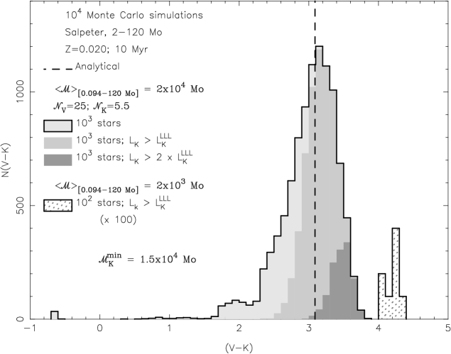
Figure 5: Probability density distribution for $V-K$ obtained from 10⁴ Monte Carlo simulations of 5.5 Myr, with 10³ stars in the mass range 2–120 M_⊙ (which corresponds to $\cal M$=2$\times 10^{4}$ in the mass range 0.094–120 M_⊙). The $V-K$ distribution for different cutoffs in $L_{K}$ is shown by different shadings (see text). The distribution for clusters with 10² stars $L_{K}>L_{K}^{LLL}$ is also shown.

In Figure 5 we described the $V-K$ distribution of a sample of model clusters with fixed number of stars, and noted that such distribution is negatively skewed. Note that a fixed number of stars correspond roughly to a fixed cluster mass. Now, let us consider only the subset of clusters with a luminosity larger than the LLL in $K$, $L_{K}^{LLL}$. This subset is shown by the light-shaded histogram, and it can be seen that its mean color is somewhat redder than the predictions of SSP models. The key point here is that this behavior indicates that the statistics of the clusters is low: in fact, at $t=10$ Myr an important fraction of the luminosity in $V$ is provided by MS stars, whereas the luminosity in $K$ is completely dominated by RSGs, which are intrinsically scarcer than MS stars. Therefore the spread in $K$ among the clusters of the sample is comparatively large, and a cutoff in luminosity, leaving out the faintest clusters, sensibly alters the mean $K$ value of the remaining subset. Schematically, we can say that in $L_{K}$ limited samples the mean $K$ luminosity increases and the $V$ luminosity is barely affected, thus $V-K$ increases. This is confirmed by the application of the more restrictive constraint $L_{K}^{clus}>2\times L_{K}^{LLL}$, which is shown by the dark-shaded histogram: the number of clusters that fulfill this constraint is even lower, and they are redder than the predictions of SSP models.

So far for clusters with (roughly) the same mass. Now, let us consider the behavior of simulated clusters with different masses. To this aim, we will assume in the following that the distribution of cluster masses follows the law $\psi({\cal M})\propto{\cal M}^{-2}$, as proposed by Zhang & Fall (1999). Whether this mass distribution correctly represents real clusters does not concern us for the moment: for the sake of the argument, it is enough to assume just any law. In fact, at the end of this section we will mention a possible caveat of this particular law, which might possibly imply a bias in the method used to derive this law. We have performed 10⁴ Monte Carlo simulations of clusters with 10² stars (${\cal M}=2\times 10^{3}$ M_⊙), which have a mean mass roughly 1/10 that of the simulated clusters discussed up to now. Given the mass distribution law assumed, we have multiplied each bin by 100, to reproduce the expected number of clusters with this mass compared with clusters with mass ten times larger.

The dotted histogram in Figure 5 shows the distribution of those of such clusters that also fulfill the condition $L_{K}^{clus}>L_{K}^{LLL}$. Note that the histogram peaks around $(V-K)^{clus}=4.2$, i.e. these clusters have extremely red colors; these behavior is consistent with the interpretation of being an effect of sampling, which in clusters of 10² stars is much more severe than in clusters of 10³ stars.

This argument can be repeated for cluster samples of any mass value. If we extrapolate the result to a continuous cluster mass distribution, we readily realize that the resulting histogram will have a cutoff in the blue (small $V-K$ values), and a long tail in the red (large $V-K$ values): i.e., it will be positively skewed, contrarily to the histogram of a complete (non-luminosity limited) sample of clusters with a fixed mass. Generalizing to different colors, the observed distribution of colors in a luminosity-limited sample will be skewed toward the band with the lowest ${\cal N}^{ssp}$ value.

Two main conclusions can be drawn from these results. First, the shape of the color distribution of a luminosity-limited sample of clusters may be used to constrain the underlying cluster mass distribution, if other cluster parameters, such as age and metallicity, are known. To this respect note the particular shape emerging from an extrapolation of our example to more mass values is just a consequence of having assumed a particular mass distribution law: in an observed sample, the shape may in principle be different. Second, these results also show that the LLL is an useful (probably, too conservative) criterion to detect the clusters with severe sampling effects. Indeed, in our examples the color of the subsets with $L_{K}^{clus}>L_{K}^{LLL}$ is different from that of the complete set, indicating that the sample suffers from sampling effects: had the mean mass of the clusters in the sample been sufficiently larger, no clusters would have been excluded by the luminosity criterion. Note also that the fact that the application of the luminosity cutoff changes the mean color of the sample implies that all the clusters of the sample suffer from incomplete sampling, and not only those that are excluded: that is, having a luminosity larger than the LLL is a condition necessary but not sufficient for the meaningful application of synthesis models; Equivalently, the LLL criterion detects some, but not all, of the clusters with poor statistics.

To conclude this section, a note of caution about the determination of the mass distribution law by Zhang & Fall (1999): these authors derived their law by considering only clusters with $M_{V}$ brighter than -9 to avoid contamination of the sample by individual stars, hence applying a selection criterion that is more or less the observational counterpart of the LLL method. However, the $M_{V}^{min}$ we obtain here for the age range they consider (2.5 $<t<$ 6.3 Myr) lies between -10 mag and -9 mag: therefore, their analysis could possibly be affected by the sampling effects and the bias we are discussing.

4.1 The distribution of Globular Clusters

A clear example of a skewed distribution is given by the sample of Globular Clusters (GCs) by (Gebhardt & Kissler-Patig 1999), a fact suggesting that the properties of these objects might be affected by sampling effects. This statement might seem surprising, for GCs are the paradigm of well-populated objects; stars in GCs occupy the most populated part of the IMF, so one would naively conclude that they cannot be possibly affected by sampling effects. However, the importance of sampling effects does not only depend on the absolute number of stars in a given mass range, but also on the evolutionary time scale considered: indeed, globular clusters also contain bright stars in low-populated evolutionary phases, such as the RGB and AGB phases. Hence sampling effects may also show up at old ages.

Let us illustrate the problem by the application of the LLL to GCs in NGC 5128. Rejkuba (2001) presents detailed photometry of GCs in NGC 5128. We have used the result from this author because her plots can be easily reproduced with the data and the indications given in the paper. She compares the position of the GCs in color-color diagrams with the results of synthesis models, and notices that the clusters lie slightly to the right and below the model lines in the $V-K$ vs. $U-V$ plane. She mentions two possible explanations: (i) a difference between observations and SSP models, particularly significant in $U-V$, which has been hypothesized by Barmy & Huchra (2000) as a consequence of problems in the atmosphere libraries used by synthesis models (see also Buser & Kurucz 1978); (ii) an additional offset may arise from the difference between the Bessell and the Johnson $U$-band transmission curves. These facts might explain the offsets between SSP models and the mean color of the observations, but they do not explain neither the observed dispersion nor the shape of the distribution. Let us now study these discrepancies when the LLL is taken into account.

Following Rejkuba (2001), we have assumed a distance modulus of 27.8 and we have corrected for extinction the observed photometric bands with a mean $E(B-V)=0.1$ using $A_{U}=4.40$, $A_{V}=3.1$, $A_{K}=0.38$, according to the values quoted in the ADPS project (Moro & Munari 2000). We have grouped the GCs according to their $L_{K}^{clus}$ luminosities: $L^{clus}_{K}/L^{LLL}_{K}<5$, $L^{clus}_{K}/L^{LLL}_{K}\in[5,10]$, $L^{clus}_{K}/L^{LLL}_{K}\in[10,30]$, and $L^{clus}_{K}/L^{LLL}_{K}>30$. We have used the $L_{K}^{LLL}$ value at 1 Gyr, that corresponds to $M_{K}^{min}=-8.5$ mag. The resulting color-color diagram is shown in Fig. 6. The results of SSP models from Worthey (1994) have also been plotted for comparison. Note that a rigorous comparison should include the confidence intervals for the results of SSP models; however, this would require knowledge of the correlation coefficients between the different luminosities, which, unfortunately, have only been evaluated for the case of young stellar populations (see Cerviño 2003d; Cerviño et al. 2002b).

Figure 6: Color-color diagram for Globular Clusters in NGC 1528. Crosses correspond to clusters with $L^{clus}_{K}/L^{LLL}_{K}>30$ ($t$= 1 Gyr); triangles to $L^{clus}_{K}/L^{LLL}_{K}\in[10,30]$; stars to $L^{clus}_{K}/L^{LLL}_{K}\in[5,10]$; and squares to $L^{clus}_{K}/L^{LLL}_{K}<5$. Small asterisks corresponds to Worthey (1994) models for all the ages and metallicities quoted by the author.

The figure shows several interesting results. First of all, the cluster sample tends to have $V-K$ colors redder than the predictions of SSP models, as is expected from a luminosity limited survey. Second, there is a statistical trend of the position in the plane with the $L_{K}$ value: (i) The first bin of clusters, the one with $L^{clus}_{K}/L^{LLL}_{K}<5$, contains five of the 23 clusters plotted, and one of them is the cluster that disagree the most with the SSP results. (ii) Of the twelve clusters with $L^{clus}_{K}/L^{LLL}_{K}\in[5,10]$, five disagree with the results of synthesis models. (iii) There are four clusters with $L^{clus}_{K}/L^{LLL}_{K}\in[10,30]$, and only one of them falls far from the results of SSP models. (iv) The two clusters with $L^{clus}_{K}/L^{LLL}_{K}>30$ are reproduced reasonably well by SSP models. In summary, clusters with lower $L_{K}$ tend to deviate more from SSP models than luminous clusters, as can be expected when sampling effects are present.

5 Caveats about self-consistency and limitations

In the present work we have established a luminosity limit, the LLL, for the application of synthesis models to observed clusters. The definition we chose for the LLL might raise objections, in at least two different ways. First, the LLL is implicitly defined by the isochrones and the atmosphere libraries assumed in the code; a natural doubt is therefore whether assuming different input libraries in the code would change our results. Second, there are evolutionary phases that are characterized by extremely high luminosities and short lifetimes. According to our definition, it is these phases that determine the value of the LLL, at the ages they occur; nevertheless, they have a very small probability of being observed in real clusters. Therefore we face the apparent oddity of setting a limit much more restrictive than necessary.

This section is devoted to clarify these points and to convince the reader that our definition of the LLL is operationally good and, to a satisfactory extent, physically based. We will also discuss its residual degree of arbitrariness, and the limitations it implies. Finally, we will also explain why, by virtue of its limited reach, the exact definition of the LLL is not very crucial in practice.

5.1 Dependence on input isochrones and model atmospheres

A possible objection to our definition of the LLL is that it depends on the input libraries (isochrones and atmosphere models) assumed by the synthesis code, suggesting that it is not physically grounded. For example, the LLL can be lowered if some stages of stellar evolution are not included in the computations of the synthesis code, as is often the case for the Asymptotic Giant Branch (AGB) phase, which is neglected, e.g., in starburst-oriented codes such as the code by Cerviño & Mas-Hesse (1994) and starburst99 (Leitherer et al. 1999). Obviously, the results of evolutionary synthesis models become intrinsically incomplete at the ages where the evolutionary stages neglected are relevant; in the case of the AGB phase, ages older than 50 Myr. Therefore, under these circumstances the concept of LLL cannot be applied, not because it is ill-defined, but rather because the code should not be used in the first place.

Furthermore, the agreement shown in Fig. 4 between the trend of our predictions for ${\cal M}^{min}$ and the ${\cal M}_{10\%}$ values by various authors, which have been obtained with different isochrones and atmosphere libraries, suggests that the LLL value does not substantially depend on the input libraries assumed - provided they include the same evolutionary stages. This conclusion should not surprise too much, since the results of different theoretical models in the fields of stellar evolution and atmosphere modeling are substantially converging. It must be noted, however, that it should not be of great concern even if this were not the case, since at the LLL level one must only worry about self-consistency, i.e. that the LLL is taken from the same input libraries that enter the synthesis code; the judgment on the input data quality has already been made with the choice of the synthesis code. Stated otherwise, the choice of a synthesis model is logically prior to the computation of the LLL, and it already implies trusting the input data the model is based on.

5.2 Dependence on short, very luminous evolutionary phases

Some readers may have noted that our definition does not involve stellar lifetimes, but just their luminosities. Such a definition might seem too restrictive in those evolutionary phases characterized by very luminous but short-lived objects: Supernovae (SNe), luminosity peaks of Luminous Blue Variable stars, and recurrent He-shell flashes in TP-AGB stars are cases in point. Due to their short duration, the probability of observing such phases in real clusters is vanishingly small, and they do not usually contribute to the observed luminosities. Yet, from a theoretical standpoint these phases provide the maximum luminosity: hence they determine the LLL value at the corresponding ages. Therefore, it may seem that our definition is at risk of giving too much weight to luminous, short-lived evolutionary phases; if this were the case, the definition would be too restrictive, and it would mistakenly ban the application of synthesis models to cases where they would otherwise be applicable. Although correct in principle, this conclusion does not hold in practice, as we will make clear in the following.

First, very short evolutionary phases are not usually included in isochrones, due to the same reason for which they should not determine the LLL: they are not expected to be observed. Of course, this argument would no longer be valid should these rapid phases be included in isochrones: but users of synthesis models should always take the elementary caution of documenting themselves about the properties, assumptions, and limitations of the models they use.

Second, it is not easy finding cutoff criteria alternative to the LLL and equally easy to apply, to discriminate systems with poor statistics from systems with good or unknown statistics. An alternative definition could be based, for example, on the comparison of the cluster luminosity with the sum of the luminosities of all the individual stars included in the isochrone (rather than the most luminous one alone, as in our definition). Unfortunately, such criterion depends on the mass resolution - the number of points - of the isochrone, which in turn depends on the individual, idiosyncratic interpolation philosophy of each code. Therefore, such definition would yield profoundly different results for different codes, even if the same set of isochrones and atmosphere libraries were adopted. Still another definition could rely on the energy emitted by a star during a particular phase, rather than its luminosity, in order to avoid the problem that arises with very luminous but short stellar phases. However, it can be seen that in this case the limit depends on how evolutionary phases are defined. For example, two possible alternatives would be either (i) “standard” evolutionary phases (e.g., Wolf-Rayet, RSG, AGB stars, and so on), or (ii) the interval around each point on the isochrone. In either case, the numerical result would depend on the adopted definition of evolutionary phase, hence on an arbitrary choice.

As a final remark, it should be emphasized that neither the LLL nor ${\cal M}^{min}$ define the statistics and the confidence levels of synthesis models, which are defined, for example, by the ${\cal N}$ formalism. In this sense, the LLL is just a two-state switch that indicates whether in each given case a statistical approach is mandatory; if it is not, it is still possible that sampling effects do play a role. In epidemiological terms, the LLL criterion is extremely specific, but not very sensitive: it does not give false positives (“good” clusters with rich statistics misunderstood for “bad” clusters with poor statistics), but it might give many false negatives (“bad” clusters with poor statistics not identified). As such, it gives a much more basic information than ${\cal N}$, hence it is not too worrisome whether its definition has a certain degree of arbitrariness. Ideally, the predictions performed by any synthesis code should be accompanied by a statistical analysis of the system under study, bypassing the need to resort to coarse indicators like the LLL.

6 Summary and conclusions

In this paper, we have drawn the attention to a basic condition that must be fulfilled in order to interpret observed stellar clusters by means of synthesis models:

The total luminosity of the cluster modeled must be larger than the individual contribution of any of the stars included in the model.

In particular, the luminosity of the most luminous star included in the model defines a Lowest Luminosity Limit below which a cluster suffers from severe sampling effects, and it cannot be modeled by an analytical synthesis code. We have emphasized that, although our method does not recognize all the clusters affected by sampling effects, by virtue of its simplicity it can be used to separate out the most critical cases from large surveys without the need to perform a sophisticated and time-consuming statistical analysis. Transient events must be considered in the LLL only if they are included in the results of SSP computations; if they are not included, the definition of the LLL is fully meaningful, under the assumption that such events are not present in the observations. Although this assumption might seem, at first glance, a very restrictive one, it does not in fact limit the application of synthesis models, since the SSP results themselves are also only valid under the same assumption.

We have obtained the Lowest Luminosity Limit for a wide range of ages and metallicities. In turn, the Lowest Luminosity Limit has been used to obtain the associated mass limit ${\cal M}^{min}$, which is the cluster mass below which the colors may be severely biased with respect to the results of synthesis models. The limit depends on the age and the metallicity of the cluster and is more stringent in the near infrared bands; in particular, it has a value between 10⁴ and 10⁵ M_⊙ for $K$. We have also shown that the luminosities in different bands of clusters with mass ten times larger than ${\cal M}^{min}$ have relative dispersions of 10% at least: that is, ${\cal M}^{min}$ can be used to estimate a lower limit to the expected dispersion of luminosities

As observational applications, we have shown that in surveys that reach luminosities near the Lowest Luminosity Limit the color distributions will be skewed toward the luminosity with the lowest ${\cal N}^{ssp}$ value, and that the skewness may be used to constrain the distribution of initial cluster masses ${\cal M}$, provided the other relevant cluster parameters are known. We have also analyzed a sample of Globular Clusters in NGC 5128, showing that sampling effects are probably playing a role, and that they can explain, at least partially, the bias of the observed colors with respect to the predictions of synthesis models.

Finally, we have discussed the assumptions underlying our definition of the LLL, its virtues, and its drawbacks. In particular, on the positive side we have stressed the extreme simplicity of the LLL as a criterion to recognize in an economical way the occurrence of poor statistics in observed clusters; on the negative side, we have highlighted the limited capability of the LLL criterion to recognize all the cases of poor statistics.

The preceding results have been obtained from very basic concepts implicit in the modeling performed by synthesis codes. In particular, the definition of the LLL is very simple, and its computation can be as elementary as finding a maximum in a table, at least in the case of SSP models. But this simplicity may be deceiving, for simple as the concept may be, it has far-reaching consequences, which have been too often overlooked in the analysis of stellar clusters. Furthermore, although the simplicity of the concept presented here might disappoint those who are fond of spectacular or complicated results, we consider it as an asset rather than a drawback, since the simplicity of our method may serve as an incentive to those who realize the importance of sampling effects but do not know how to deal with them. Therefore, our aim in the present work is twofold and goes beyond the particular results we have described in this paper: in the short term, we want to provide a very simple sieve to detect rapidly clusters with poor statistics; in the long term, we hope to motivate other researchers, both theoreticians and observers, to move in this direction and explore the implications of sampling effects in the analysis of the integrated light from clusters. In particular, we urge all the model makers to include a proper statistical treatment in their code, and all the model users to take into account the effects of sampling in the interpretation of the data. Current synthesis models are an optimum tool for the interpretation of the average properties of stellar systems, but they need to be updated to keep pace with the new observational data.