Red galaxy overdensities and the varied cluster environments of powerful radio sources with $\mathbf{z\sim 1.6}$

Abstract

The environments of a complete subsample of 6 of the most powerful radio–loud AGN at redshifts $z\sim 1.6$ are investigated, using deep $RJK$ imaging to depths of $R\sim 26$, $J\sim 22.4$ and $K\sim 20.6$. An excess of galaxy counts in the K–band is seen across these fields; these surplus galaxy counts are predominantly associated with red galaxies ($R-K\mathrel{\hbox to0.0pt{\lower 3.0pt\hbox{$\mathchar 536\relax$}\hss}\raise 2.0pt\hbox{$\mathchar 318\relax$}}4$) of magnitudes $17.5\mathrel{\hbox to0.0pt{\lower 3.0pt\hbox{$\mathchar 536\relax$}\hss}\raise 2.0pt\hbox{$\mathchar 316\relax$}}K\mathrel{\hbox to0.0pt{\lower 3.0pt\hbox{$\mathchar 536\relax$}\hss}\raise 2.0pt\hbox{$\mathchar 316\relax$}}20.5$ found within radial distances of $\sim$1 Mpc of the AGN host. These are exactly (though not uniquely) the magnitudes, colours and locations that would be expected of old passive elliptical galaxies in cluster environments at the redshifts of these AGN. Using both an Abell–style classification scheme and investigations of the angular and spatial cross–correlation functions of the galaxies, the average environment of the fields around these AGN is found to be consistent with Abell cluster richness classes 0 and 1. The amplitude of the angular cross-correlation function around the AGN is shown to be a strong function of galaxy colour, and is highest when only those galaxies with the colours expected of old elliptical galaxies at these redshifts are considered.

The images cover a relatively wide field, 5 by 5 arcmins, allowing the distribution of the surplus galaxy counts to be investigated. The galaxy overdensities are found on two scales around the AGN: (i) pronounced central concentrations on radial scales within $\sim 150$ kpc; where present, these are composed almost entirely of red ($R-K\mathrel{\hbox to0.0pt{\lower 3.0pt\hbox{$\mathchar 536\relax$}\hss}\raise 2.0pt\hbox{$\mathchar 318\relax$}}4$) galaxies, suggesting that the morphology–density relation is imprinted into the centres of clusters at a high redshift. (ii) weaker large–scale excesses extending out to between 1 and 1.5 Mpc radius. The presence or absence of galaxy excesses on these two scales, however, differs greatly between the six different fields: the fields of two AGN do show red galaxy excesses on both scales, another two fields show only a large–scale red galaxy overdensity with no pronounced central concentration, and one field shows only a sharp central peak of red galaxies with no large–scale overdensity. The final field shows little evidence for an excess on any scale; this field is associated with an unresolved radio source, perhaps indicating that only extended radio sources probe cluster environments.

Clearly there is a large range in both the richness and the degree of concentration of any clustering environments around these distant AGN. The implications of this for both cluster formation and the nature of high redshift AGN are discussed.

1 Introduction

Understanding the formation of large scale structure and the related formation and evolution of galaxies are two of the most important issues in modern–day astronomy. Rich clusters of galaxies at high redshifts ($z\mathrel{\hbox to0.0pt{\lower 3.0pt\hbox{$\mathchar 536\relax$}\hss}\raise 2.0pt\hbox{$\mathchar 318\relax$}}1$) provide an opportunity to investigate both of these problems directly: first, since clusters are the largest, most massive, collapsed structures in the Universe, discerning the epoch and process of their assembly places strong constraints on models of large scale structure formation (e.g. Bahcall & Fan 1998); second, because they contain large numbers of galaxies at the same distance, clusters provide a unique resource for investigating galaxy evolution through the evolution of galaxy scaling relations such as the fundamental plane (e.g. van Dokkum et al 1998) and colour–magnitude relations (e.g. Stanford et al. 1998); third, clusters contain the oldest galaxies known, and these can strongly constrain the first epoch of formation of ellipticals (cf Dunlop et al. 1996, Spinrad et al. 1997).

The identification of significant samples of clusters much above redshift one is both challenging and inefficient using optical or X–ray selection techniques. Existing X–ray surveys suffer from sensitivity limits (the ROSAT Deep Cluster Survey, for example, found very few clusters above $z\sim 1$, and none above $z=1.3$; e.g. Stanford et al. 2002) whilst the smaller field of view of the current generation of X-ray telescopes make them relatively inefficient for wide–area surveys. At optical wavelengths the contrast of a cluster above the background counts is minimal above redshift one, requiring very deep wide–area multi–colour surveys including near–infrared wavebands to identify a significant sample of $z\gg 1$ clusters; whilst certainly feasible, this is very expensive on telescope time. For this reason, an alternative method has frequently been adopted, using targetted studies towards powerful AGN. At low redshifts AGN are frequently found in relatively rich environments (e.g. Yates, Miller and Peacock 1989; Hill & Lilly 1991), and the host galaxies of high redshift AGN are amongst the most massive galaxies known in the early Universe (e.g. de Breuck et al. 2002), making these promising candidates for residing in galaxy overdensities.

The environments of powerful radio sources at redshifts $z\sim 1$ have been investigated by many authors over recent years using a variety of different techniques, including searches for luminous extended X–ray emission (e.g. Crawford & Fabian 1996; Fabian 2001), searches for over-densities of galaxies in infrared colours (e.g. Dickinson 1997, Hall & Green 1998) or emission line images (e.g. McCarthy et al. 1995), investigations of the colour–magnitude relations for red cluster ellipticals (e.g. Best 2000, hereafter B00), cross–correlation analyses (e.g. B00; Wold et al 2000) and direct spectroscopic studies of individual sources (e.g. Dickinson 1997, Deltorn et al. 1997). The evidence that at least some powerful $z\sim 1$ radio sources are located at the centres of galaxy overdensities is overwhelming (see B00 for a review). What remains unclear is the ubiquity, scale, and nature of these (proto?) clusters.

At higher redshifts, radio sources have been detected out to $z=5.2$ [1999], and some well–studied sources have been spectroscopically confirmed to lie in overdense environments (e.g. 1138-215 at $z=2.2$; Kurk et al. 2000; Kurk et al. in preparation). An on–going VLT large project (PI: Miley) has found order–of–magnitude overdensities of Ly-$\alpha$ emitters around all 4 deeply studied $z>2$ radio galaxies to date (Venemans et al. in preparation), including the detection of the most distant known large structure around the $z=4.1$ radio galaxy TN J1338-1942 [2002]. The $\sim 20$ line emitting galaxies in the structures around each of these high redshift radio galaxies are found over regions extending to $\mathrel{\hbox to0.0pt{\lower 3.0pt\hbox{$\mathchar 536\relax$}\hss}\raise 2.0pt\hbox{$\mathchar 318\relax$}}3$ Mpc, and have velocity dispersions of 300–1000 km s ^-1(Venemans et al., private communication). Thus, it does indeed seem that powerful radio galaxies offer unique prospects for tracking galaxy clusters over cosmic time. The detection of overdensities at these redshifts, however, is based predominantly on observing emission–line galaxies near the radio galaxy redshift; the strong red sequences characteristic of nearby clusters are not observed towards these $z>2$ overdensities, restricting the evolutionary studies of cluster ellipticals using the fundamental plane and colour–magnitude relations from being extended to these high redshifts.

The redshift range $1.2\mathrel{\hbox to0.0pt{\lower 3.0pt\hbox{$\mathchar 536\relax$}\hss}\raise 2.0pt\hbox{$\mathchar 316\relax$}}z\mathrel{\hbox to0.0pt{\lower 3.0pt\hbox{$\mathchar 536\relax$}\hss}\raise 2.0pt\hbox{$\mathchar 316\relax$}}2.0$ is therefore a particularly interesting redshift range to study. This is the redshift range where cluster studies go beyond those currently being carried out using optical and X–ray selected clusters, whilst still being of low–enough redshift that red sequences of cluster ellipticals are likely to exist, and can be studied in a practical amount of observing time. Such clusters will also allow a link to be made between the ‘proto’-clusters being found around $z>2$ radio galaxies, and the rich virialised clusters seen in the nearby Universe. The elliptical galaxy population in clusters may well be undergoing a fundamental change within this redshift range

Hall & Green [1998] have previously investigated the small–scale environments of a sample of 31 quasars with redshifts $1\mathrel{\hbox to0.0pt{\lower 3.0pt\hbox{$\mathchar 536\relax$}\hss}\raise 2.0pt\hbox{$\mathchar 316\relax$}}z\mathrel{\hbox to0.0pt{\lower 3.0pt\hbox{$\mathchar 536\relax$}\hss}\raise 2.0pt\hbox{$\mathchar 316\relax$}}2$, variably selected from previous surveys. They found an excess of K–band galaxy counts on two scales around the quasars; a pronounced peak in the galaxy counts within the central 40 arcsec radius surrounding the quasars was accompanied by a uniform galaxy overdensity across their entire fields (to about $\sim 1.5$ arcmins radius). Comparing R and K–band data they showed that the excess counts correspond to redder galaxies than the typical field population, with a significant overdensity of extremely red objects. This is indicative that a red elliptical sequence may be present in these fields. Hall et al. [2001] investigated the physical extent of the large–scale overdensity in the fields of two of these AGN, and found a net excess of galaxy counts out to 140 arcsec ($\sim 1.3$ Mpc) in one of the two fields.

We have embarked upon a project to investigate in detail the environments of a complete sample of the most luminous radio sources (radio galaxies and quasars) within the narrow redshift range $1.44\leq z\leq 1.7$. The aim of this project is to use deep, wide–area multi–colour imaging to study in detail any galaxy overdensity, in particular the nature of the excess galaxies, the presence of a red sequence of cluster ellipticals, and the radial extent of the overdensity. By studying a complete AGN sample it will be possible to investigate the variety of environments found, and whether the environment of a radio–loud AGN is in any way correlated with the radio source properties. The candidate cluster galaxies in the richest overdensities can then be followed–up using multi–object spectroscopy in order to extend the galaxy evolution studies.

This paper provides the initial results of this project, focussing on the imaging data and results from the first 6 clusters in the sample. Specifically, the lay-out of the paper is as follows. In Section 2 the sample selection, observations, and data reduction are described. The resulting multi–colour images of each field are provided and described in Section 3, and galaxy catalogues are constructed from these. The galaxy number counts and the colour distribution of the galaxies are investigated in Section 4, and a cross–correlation analysis carried out. The properties of the different fields are related to the properties of their AGN in Section 5. The results are discussed and conclusions drawn in Section 6. Throughout the paper, the values adopted for the cosmological parameters are $\Omega_{\rm M}=0.3$, $\Omega_{\Lambda}=0.7$ and $H_{0}=65$ km s^-1Mpc^-1.

2 Observations

2.1 Sample Selection and Observations

The radio sources were drawn from the equatorial sample of 178 powerful radio sources defined by Best, Röttgering and Lehnert (1999; the BRL sample). This sample was designed to be equivalent to the northern 3CR sample, and was drawn from the Molonglo radio survey at 408 MHz [1981], according to three criteria: (i) the sources must have declinations $-30^{\circ}<\delta<+10^{\circ}$; (ii) they must lie away from the galactic plane, $|b|>10$; (iii) they must be brighter than $S_{\rm 408MHz}=5$ Jy (roughly equivalent to the definition of the 3CR sample). Spectroscopic redshifts are available for 177 of these 178 sources [1999, 2000].

From the BRL sample, the 9 radio sources with redshifts $1.44\leq z\leq 1.7$ and galactic latitudes $|b|>25$ were selected. This sample comprised 4 radio galaxies and 5 radio loud quasars. Of these, the environments of 6 radio sources have been studied to date, and are presented in this paper. These 6 radio sources, limited by the constraints of telescope time, correspond to all of those with $15<{\rm RA}<02$ and therefore constitute a complete subsample of the most powerful radio sources at these redshifts.

The aim of the current observations was to deeply image these fields in the $R$, $J$ and $K$ wavebands. This filter combination was chosen to provide maximal sensitivity to old cluster ellipticals: the strongest continuum features of such ellipticals is the 4000Å break, which at $z\sim 1.5$ falls between the $R$ and $J$ bands, making this colour very sensitive to old cluster galaxies. The addition of the $K$–band data provides a long red colour baseline to sample the old stellar populations of these ellipticals, whilst also facilitating identification of bluer cluster galaxies with on-going star formation (and hence less pronounced 4000Å breaks), and helping to filter out non–cluster objects with very red $R-J$ colours, such as dusty starbursting galaxies. At $z\sim 1.5$ passively evolving old ellipticals would have colours of $J-K\sim 1.8$ and $R-J\sim 3.7$, and brightest cluster galaxies at these redshifts are expected to have magnitudes of $K\sim 17.5$ to 18 (cf. those of radio galaxies at these redshifts, e.g. Best et al. 1998). The goal of detecting elliptical galaxies in all colours to $\sim 3$ magnitudes fainter than this set the required depths of the different observations. Full details of the observations are provided in Table 1.

The six fields were observed in the $J$ and $K$–bands using the infrared imager SOFI on the ESO New Technology Telescope (NTT) during September 2000 and August 2001. SOFI has a 1024 by 1024 HgCdTe array with 0.29 arcsec pixels, providing a field of view of 5 by 5 arcmins. Images were taken using a jittering technique, with the pointing centre moved randomly within a 40 arcsec square box between each exposure. At each pointing position, 1–minute of data was taken, split into six 10s co-adds in the K–band and three 20s co-adds in the J–band. In the $K$–band the $K_{s}$ filter was used to reduce the sky background; the $K_{s}$ magnitude is related to the $K$-magnitude by $K-K_{s}\approx-0.005(J-K)$, and all quoted magnitudes have been converted to the $K$–band magnitude. Between 1.7 and 2.5 hours of data were obtained for each source (see Table 1 for details), reaching a ‘limiting magnitude’ of $K\sim 20.6$; this value corresponds to the 50% completeness limit for galaxies with sizes typical of those at redshifts $z\sim 1.6$. In the $J$–band the total exposure time varied between 1 and 2 hours, reaching a limiting depth of $J\sim 22.4$.

For 5 of the 6 fields (2128$-$208 was randomly excluded due to telescope time constraints), $R$-band data for the field were taken through the Bessel $R$ filter using SUSI-2 on the NTT. SUSI-2 comprises two 2048 by 4096 pixel EEV CCDs, with a pixel scale of 0.08 arcsec, which combined provide a 5.5 by 5.5 arcminute field of view. The two CCDs are separated by about 10 arcseconds on the sky; the total exposure time was therefore separated into 5-min blocks, with the pointing position moved through a 9-point pattern of offsets [(0,0), (10,10), (20,-10), (30,0), (40,10), (-40,-10), (-30,0), (-20,10), (-10,-10) arcsec] in order to attain equal sensitivity over the entire SOFI field. This pattern was repeated until between 3.75 and 6 hours of data had been obtained on each field, reaching a limiting depth of $R\sim 25.9$.

Standard stars were observed approximately every 2 hours throughout the nights to allow the images to be photometrically calibrated. For the SUSI-2 images, once each night the image was rotated by 180 degrees in order to place the standard stars on the opposite CCD; no significant differences in calibration were apparent between the two CCDs. All of the nights were photometric, and the instrument zero-points varied by less than 0.05 magnitudes within each of the Sept 2000 and Aug 2001 runs, although the $R$–band zero point changed by 0.1 magnitudes between the two runs.

Table 1: Details of the observations.

Source	RA	Dec	z	Waveband	Obs.	Telescope	Exp.	Mean	Limiting
	J2000				Dates	&	Time	Seeing	Magnitude∗
						Instrument	[mins]	[arcsec]
MRC 0000-177	00 03 21.93	$-$17 27 11.9	1.47	$K_{s}$	2001 Aug 10,12	NTT-SOFI	138	0.98	20.4
				J	2001 Aug 11,12	NTT-SOFI	120	1.01	22.3
				R	2001 Aug 12	NTT-SUSI2	270	1.00	25.8
MRC 0016-129	00 18 51.36	$-$12 42 34.4	1.59	$K_{s}$	2000 Sep 23	NTT-SOFI	103	0.62	20.7
				J	2000 Sep 23,25	NTT-SOFI	60	0.80	22.3
				R	2000 Sep 20,24,25	NTT-SUSI2	225	0.85	25.8
MRC 0139-273	01 41 27.31	$-$27 06 11.1	1.44	$K_{s}$	2000 Sep 23,25	NTT-SOFI	135	0.64	20.6
				J	2000 Sep 23,25	NTT-SOFI	105	0.74	22.6
				R	2000 Sep 20,24,25	NTT-SUSI2	360	0.74	26.1
MRC 1524-136	15 26 59.45	$-$13 51 00.2	1.69	$K_{s}$	2001 Aug 10,11	NTT-SOFI	135	0.80	20.5
				J	2001 Aug 10	NTT-SOFI	105	0.90	22.4
				R	2001 Aug 11,12	NTT-SUSI2	255	1.15	25.5
MRC 2025-155	20 28 07.68	$-$15 21 20.9	1.50	$K_{s}$	2000 Sep 20,23	NTT-SOFI	114	0.75	20.4
				J	2000 Sep 23	NTT-SOFI	91	0.90	22.3
				R	2000 Sep 24,25	NTT-SUSI2	260	0.65	25.9
MRC 2128-208	21 31 01.49	$-$20 36 56.4	1.62	$K_{s}$	2001 Aug 10	NTT-SOFI	150	0.77	20.6
				J	2001 Aug 10	NTT-SOFI	105	1.00	22.5

^∗ The ‘limiting magnitude’ quoted is the approximately 50% completeness limit for galaxies with physical sizes typical of those in a $z\sim 1.6$ cluster.

2.2 Data reduction

The infrared observations were reduced in the standard manner, using the dimsum package within iraf. After subtraction of a dark frame, and removal of known bad pixels, a median of the images (after masking of bright objects) was constructed to obtain an accurate sky flat–field. The flat–fielded images were then sky subtracted, cosmic ray events were removed, and then the individual frames were block replicated by a factor of 2 in each dimension to allow more accurate alignment, resulting in a final image scale of 0.144 arcsec per pixel. The frames were accurately registered using the peak positions of several bright unresolved objects visible on all images, and were combined. Because of the long exposure times, the seeing sometimes varied throughout the dataset, and so during the combination process the images were weighted according to their seeing in order to provide a final image with the optimal combination of seeing and sensitivity. Stars from the US Naval Observatory catalogue A2.0 [1998] were used to provide an astrometric solution for the images. The absolute astrometry should be accurate to better than 0.5 arcsec. The fields were photometrically calibrated onto the standard Vega photometric system.

The $R$–band images were reduced within iraf. The images were bias subtracted, and then flat–fielded using a flat–field constructed by from the median of the various images (after masking bright objects). An illumination correction was then applied to remove large–scale variations in the flat–fielded images. The images were registered using the peak positions of several bright unresolved objects, and then they were combined, weighted according to their seeing as for the $J$ and $K$ band data. Cosmic rays were rejected during the combination process. The resultant image was then astrometrically transformed using a 5 parameter fit (RA and Dec of the central pixel, pixel scale in x and y directions, and rotation angle) to align it with the infrared data, converting it to 0.144 arcsec pixels whilst conserving the object magnitudes. The relative astrometry of the IR and optical frames is accurate to $<0.1$ arcsec.

3 The radio source fields

K-band images of the six fields are shown in Figures 1 to 3, with the radio source host galaxy marked by a cross in each case. Three–colour images of the 100 by 100 arcsec region around the radio source host in each field are provided in Figures 4 to 6. A brief discussion of each individual field follows.

0000–177 ($\mathbf{z=1.47}$): This radio–loud quasar lies in a relatively sparse region of sky. A faint object is seen 1-2 arcsec to the north–east of the quasar host, and a further seven objects with $R-K>4$ lie within 30 arcsec ($\approx 275$ kpc at $z\sim 1.5$), indicating a possible compact group of galaxies at the quasar redshift. There is no obvious large–scale galaxy overdensity.

0016–129 ($\mathbf{z=1.59}$): This radio galaxy is the westernmost of a string of three luminous red galaxies in the centre of this field, and shows extended blue emission along the radio axis direction, characteristic of the alignment effect in high redshift radio galaxies (cf. McCarthy et al. 1987, Chambers et al. 1987). The redder galaxies in the field are more concentrated towards the central regions of the field, within 1–2 arcmins of the AGN.

0139–273 ($\mathbf{z=1.44}$): This is the richest field of those imaged in the current observations, and contains a large number of very red galaxies. These galaxies are found predominantly within the inner regions of the field, although no red galaxies are seen close to the AGN. Very luminous elongated blue emission extends from the radio galaxy host, along the direction of the radio source axis.

1524–136 ($\mathbf{z=1.69}$): This radio loud quasar is the highest redshift AGN in the current sample, and its surrounding field is relatively rich in the K–band. A moderate excess of red galaxies is seen on scales out to about 120 arcsec ($\sim$ 1 Mpc). No sharp central peak (such as that seen for 2025$-$155) is seen, suggesting that any cluster environment may still be forming.

2025–155 ($\mathbf{z=1.50}$): A very compact group of several red galaxies is found within 15–20 arcsec (150 kpc) radius of this radio–loud quasar. All of these objects have colours consistent with old passive ellipticals at the radio source redshift. A significant overdensity of red galaxies is found extending over the entire 5 arcmin field, although predominantly within the inner regions.

2128–208 ($\mathbf{z=1.62}$): This field does not contain a particular excess of K-band galaxies and, except for a companion object to the quasar, no other galaxy is found within 15 arcsec of the AGN host. With only J and K–band data available, there is little information about the colour distribution of the galaxies across the field.

It is clear from this direct examination of the different images that a wide variety of environments in found amongst the sample. At one extreme, the field of 2128$-$208 shows little evidence for any net overdensity of red galaxies on either small ($\mathrel{\hbox to0.0pt{\lower 3.0pt\hbox{$\mathchar 536\relax$}\hss}\raise 2.0pt\hbox{$\mathchar 316\relax$}}150$ kpc) or large ($\sim$ Mpc) scales, whilst in contrast 2025$-$155 has a very rich environment on small scales coupled with an apparent excess of red galaxies across the entire field. Between these extremes, the other fields show evidence for structure on differing scales: a small scale excess of red galaxies is found around 0000$-$177, but not much large scale structure; the 0016$-$129 field has three central red galaxies and a weak larger–scale excess; above average numbers of red galaxiess are seen on both moderate and large scales around 1524$-$136; and the field of 0139$-$273 shows a strong excess of red galaxies on larger scales, but with few red objects close to the AGN. In the discussions of the statistical properties of the fields that follow, it is important to bear in mind that global results quoted correspond to the average values across 6 rather different environments.

Figure 1: [See attached jpg files] Top: The K-band image of the field of 0000$-$177 ($z=1.47$). Bottom: The K-band image of the field of 0016$-$129 ($z=1.59$).

Figure 2: [See attached jpg files] Top: The K-band image of the field of 0139$-$273 ($z=1.44$). Bottom: The K-band image of the field of 1524$-$136 ($z=1.69$).

Figure 3: [See attached jpg files] Top: The K-band image of the field of 2025$-$155 ($z=1.50$). Bottom: The K-band image of the field of 2128$-$208 ($z=1.62$).

Figure 4: [See attached jpg files] Top: An R,J,K colour image of the central 100 $\times$ 100 arcsec field around the $z=1.47$ quasar 0000$-$177. Bottom: An R,J,K colour image of the central 100 $\times$ 100 arcsec field around the $z=1.59$ radio galaxy 0016$-$129.

Figure 5: [See attached jpg files] Top: An R,J,K colour image of the central 100 $\times$ 100 arcsec field around the $z=1.44$ quasar 0139$-$273. Bottom: An R,J,K colour image of the central 100 $\times$ 100 arcsec field around the $z=1.69$ radio galaxy 1524$-$136.

Figure 6: [See attached jpg files] Top: An R,J,K colour image of the central 100 $\times$ 100 arcsec field around the $z=1.50$ quasar 2025$-$155. Bottom: A J,K colour image of the central 100 $\times$ 100 arcsec field around the $z=1.62$ quasar 2128$-$208.

3.1 The source catalogues

Source extraction and catalogue construction followed the method described in detail by B00, and the reader is referred to that paper for full details. This method is summarised briefly below.

Throughout these analyses, the K–band data were used as the primary dataset from which the catalogue is defined. Source detection and photometry were carried out on the K–band frames using sextractor version 2.2.1 [1996], using the output exposure map produced by dimsum as a weight map for sextractor to compensate for the varying noise levels associated with the jittering procedure. The source extraction parameters were set such that, to be detected, an object must have a flux in excess of 1.5 times the local background noise level over at least $N$ connected pixels, where $N$ was varied a little according to the seeing conditions, but in general was about 15 (equivalent to 4 pixels prior to the block replication during the mosaicing procedure). A search for negative holes using the same extraction parameters (cf B00) found only one negative feature over all 6 frames brighter than the 50% completeness limit, implying that essentially all of the extracted objects down to that level are real. The sextractor catalogues were examined carefully, and obvious problems, such as objects associated with the diffraction spikes of bright stars, were corrected. Those objects within the central 2000 by 2000 pixels (290 by 290 arcsec) of each image were retained for the subsequent analysis; more distant objects lie in the regions of the image where the noise levels are higher due to the jittering process, and were discarded; at the edges of the retained regions of the fields, the noise level is only $\sim 10$% higher than in the field centre. Small regions of sky (of 10, 20 and 10 arcsecond radius) were also discarded around the three bright stars in the images of 0016$-$129, 1524$-$136 and 2025$-$155. The six fields combined provide a sky area of 140 square arcminutes.

sextractor’s mag_best estimator was used to determine the magnitudes of the extracted sources; this yields an estimate for the ‘total’ magnitude using Kron’s [1980] first–moment algorithm, except if there is a nearby companion which may bias the total magnitude estimate by more than 10% in which case a corrected isophotal magnitude is used instead. sextractor isophotal apertures smaller than 1 arcsecond were replaced by circular 1 arcsecond apertures. The determined magnitudes were corrected for galactic extinction using the $E(B-V)$ values provided in the NASA / IPAC Extragalactic Database (NED). The accuracy of these total magnitudes and the completeness level of the source extraction were investigated as a function of position on each image through a Monte–Carlo simulation, as fully described by B00. Briefly, a total of 10000 stellar objects and 25000 galaxies (see B00 for the prescription by which these were constructed) were added, 25 at a time, to each image with a magnitude between 15 and 22.5, and were then re-extracted using sextractor with the same input parameters as for the original source extraction, to see if the added objects were detected. For each recovered source, the difference between the total magnitude measured by sextractor and the input total magnitude was determined.

From these results, the mean completeness fraction was determined as a function of magnitude for both stars and galaxies over the entire set of images. The mean 50% completeness limits are $K=20.55$ for galaxies and $K=21.05$ for stars (see Figure 7); the galactic completeness limits for each individual field are provided in Table 1. The mean difference between the input and measured magnitudes, and the scatter of the measured magnitudes around this mean, are shown as functions of input magnitude for both model stars and galaxies in Figure 8. This difference was used to correct the observed magnitudes and obtain true total magnitudes.

Figure 7: The completeness fraction for both stellar (dashed line) and galactic (solid line) model objects as a function of input magnitude, averaged over all 6 fields.

Figure 8: The mean (upper plot) and rms scatter (lower plot) of the difference between the measured magnitudes and input magnitudes for the model stars (dashed line) and galaxies (solid line).

The $J$ and $R$ band magnitudes for the catalogue sources were then measured by running sextractor in its double image mode, where one image (the $K$ band) is used to detect the objects and the fluxes and magnitudes are then measured from the second ($J$ or $R$ band) image through the same aperture. Those objects whose $J$ or $R$ band fluxes were measured to have a significance of less than 3$\sigma$, where $\sigma$ is the uncertainty on the flux measurement provided by sextractor, were replaced by 3$\sigma$ upper limits. The sextractor flux error estimate includes the uncertainty due to the Poisson nature of the detected counts and that from the standard deviation of the background counts. An additional source of flux error arises from the uncertainty in the subtraction of the background count level as a function of position across the image. This value was estimated as the product of the area of the extraction aperture and the rms variation of the subtracted background flux across blank regions of the image. This background subtraction error estimate was combined in quadrature with the flux error given by sextractor to determine the uncertainties on the magnitudes of the extracted objects in all three colours.

3.2 Star–galaxy separation

sextractor provides a ‘stellaricity index’ for each object, where in the ideal case a galaxy has a stellaricity index of 0.0 and a star has 1.0; low signal–to–noise, and galaxies more compact than the seeing, lead to an overlap in the calculated stellaricity indices for the two types of object at the faintest magnitudes, and hence uncertain star–galaxy separation. Stellaricity indices were taken from the K–band data. At magnitudes $K\mathrel{\hbox to0.0pt{\lower 3.0pt\hbox{$\mathchar 536\relax$}\hss}\raise 2.0pt\hbox{$\mathchar 316\relax$}}18$, star–galaxy separation could be carried out directly from these stellaricity values taking values above 0.8 (the generally adopted cut-off) to correspond to stars. At fainter magnitudes, separation is less certain, but was aided by the addition of the multi–colour information; by plotting the R-K versus J-K colour–colour diagram as a function of stellaricity index, a region of colour space typically occupied by stars was defined (see Figure 9), and all objects in this colour space region with stellaricities above 0.5 were also classified as stars. This classification is somewhat conservative, and a small proportion of stars may be included along with the galaxies, but this was considered preferable to falsely classifying galaxies as stars.

Figure 10 shows the total star counts as a function of magnitude derived from all of the frames, fit with the function $\log N(K)=0.201K-0.128$. This relatively good fit to the differential star counts using a single power–law distribution demonstrates that the star–galaxy separation is working well to at least $K\sim 20$. All objects classified as stars were removed from further analysis.

Figure 9: A set of $R-K$ versus $J-K$ colour–colour plots for objects in the field of 2025-155, separated by the stellaricity index output by sextractor. The solid lines define a region of colours separating the majority of the stellar locus from typical galactic colours. All objects with stellaricity indices greater than 0.8 were classified as stars, together with those objects with stellaricities between 0.5 and 0.8 lying to the upper left of the two lines.

Figure 10: The differential star number counts in the K–band, in $\Delta K=0.5$ magnitude intervals, fit using a single power law distribution.

4 Galaxy Counts and Colours

4.1 Galaxy counts

The galaxy counts were determined by once again following the procedure of B00. In brief, the measured magnitudes of the galaxies were converted to true ‘total’ magnitudes using the offsets determined from the simulations above, and binned in 0.5 magnitude bins over the magnitude range $14<K<21$. These raw galaxy counts, $n_{\rm raw}$, were then corrected for completeness and for magnitude biasing effects (again as calculated from the results of the simulations) to produce corrected galaxy counts ($n_{\rm c}$). Scaling by the observed sky area produced final counts per magnitude per square degree, $N_{\rm c}$. In calculating the uncertainty on this value, in addition to the Poissonian error on the raw galaxy counts, an extra error term was included to account for the uncertainty of the completeness correction procedure; this was estimated at 20% of the number of galaxies added in the correction. The resulting galaxy counts are tabulated in Table 2 and are plotted in Figure 11 compared with counts from various K–band blank–field surveys [1993, 1995, 1995, 1997, 198, 1998, 1998, 1999, 2000, 2001].

The derived counts are fully consistent with the literature counts at magnitudes $K\mathrel{\hbox to0.0pt{\lower 3.0pt\hbox{$\mathchar 536\relax$}\hss}\raise 2.0pt\hbox{$\mathchar 316\relax$}}17.5$. This magnitude corresponds to the expected magnitude of brightest cluster galaxies at $z\sim 1.5$. Fainter than this magnitude an surplus of galaxies is seen; the galaxy counts still lie within the scatter of the other observations, that scatter being largely dominated by cosmic variance (cf Daddi et al. 2000a), but the counts in every magnitude bin from $17.5<K<20.5$ exceed the literature average by at least 1$\sigma$.

Figure 11: The K–band galaxy number counts per magnitude per square degree. The solid symbols represent the data presented in this paper and tabulated in Table 2. The open symbols represent data from the literature: squares are from Minezaki et al. (1998), triangles from Djorgovski et al. (1995), diamonds from Moustakas et al. (1997), circles from Szokoly et al. (1998), x’s from Gardner, Cowie & Wainscoat (1993), asterisks from McLeod et al. (1995), inverted triangles from Bershady, Lowenthal & Koo (1998), stars from Totani et al. (2001), crosses from Väisänen et al. (2000), and bow-ties ($\bowtie$) from Saracco et al. (1999).

Table 2: K–band galaxy counts as a function of magnitude, over the combined 140 square arcminutes. The columns give the raw ($n_{\rm raw}$) and corrected ($n_{\rm c}$) counts, the corrected counts per square degree per unit magnitude ($N_{\rm c}$), the error on this, and the mean literature counts ($N_{\rm lit}$).

$K$	$n_{\rm raw}$	$n_{\rm c}$	$N_{\rm c}$∗	$\delta N_{\rm c}$∗	$N_{\rm lit}$∗
All fields
14.0 – 14.5	2	2.0	103	72	86
14.5 – 15.0	5	5.0	257	115	175
15.0 – 15.5	6	6.0	309	126	340
15.5 – 16.0	13	13.0	670	185	710
16.0 – 16.5	24	24.2	1250	250	1160
16.5 – 17.0	46	46.5	2400	350	2280
17.0 – 17.5	69	69.7	3590	440	4010
17.5 – 18.0	118	120.8	6230	580	5530
18.0 – 18.5	170	172.8	8920	690	8260
18.5 – 19.0	254	263.5	13600	860	10500
19.0 – 19.5	361	375.3	19400	1030	15300
19.5 – 20.0	476	522.9	27000	1350	23100
20.0 – 20.5	472	685.1	35300	3500	31900
20.5 – 21.0	292	927.8	47900	7400	41800
∗: counts per magnitude per square degree.

Table 3: Properties of the galaxies in the individual fields. The columns give: (1) the radio source field; (2) the K–band galaxy counts (in galaxies per square degree) between $17.5<K<20.5$, and the uncertainty of this value — this uncertainty includes both the Poissonian error and a cosmic variance term; (3) the deviation of the number counts from the mean literature counts; (4 and 5) the mean and median $R-K$ colours of these galaxies; (6) the Abell cluster strength estimator $N_{\rm 0.5}$, and its error. The bottom two rows of the table give the values average over all of the fields, and blank–field expectations for the number counts and average colours as drawn from the literature (see text for details).

Field	$N_{\rm c}$	Excess	$R-K$		$N_{\rm 0.5}$
	[deg-2]		Mean	Median
(1)	(2)	(3)	(4)	(5)	(6)
0000$-$177	$42200\pm 5100$	$-1.0\sigma$	4.19	4.19	$-3\pm 5$
0016$-$129	$55400\pm 5800$	$+1.4\sigma$	4.09	4.05	$4\pm 6$
0139$-$273	$64200\pm 6200$	$+2.7\sigma$	3.98	3.93	$18\pm 8$
1524$-$136	$59600\pm 6100$	$+2.0\sigma$	4.07	3.85	$14\pm 7$
2025$-$155	$58700\pm 5900$	$+1.9\sigma$	4.05	3.89	$11\pm 7$
2128$-$208	$50400\pm 5600$	$+0.6\sigma$	—	—	$3\pm 6$
Combined	$55000\pm 2400$	$+3.1\sigma$	4.08	3.95	$8\pm 3$
Literature	$47500\pm 2000$	—	3.87	3.78	—

In Table 3 the total galaxy counts in the magnitude range $17.5<K<20.5$ are provided for each individual field, and compared to the mean value of the blank–field surveys. To carry out such a comparison it is important to bear in mind that the uncertainty on the counts in the AGN fields will be significantly larger than solely the Poissonian error, due to cosmic variance and the effects of galaxy clustering. The true uncertainty on the counts can be estimated from the equation $\sigma_{\rm true}^{2}=N(1+NAC)$, where $N$ is the total counts, $A$ is the angular cross–correlation amplitude, and $C$ is the integral constraint which depends upon the size and geometry of the field. As derived in Section 4.6, for these fields the values of $A$ and $C$ are 0.0005 and 16.7 respectively. Hence, for $N\sim 300$ galaxies detected in each field, the uncertainty on the counts is approximately double that which would be expected from Poissonian statistics alone. The errors tabulated in Table 3 are these true errors, including this contribution of cosmic variance. For the literature counts, given that these are derived by combining many independent surveys over different areas of sky, the combination should average out the cosmic variance effects to a large extent.

It is noteworthy that five of the six fields have counts above the literature average, with three of the fields being $\mathrel{\hbox to0.0pt{\lower 3.0pt\hbox{$\mathchar 536\relax$}\hss}\raise 2.0pt\hbox{$\mathchar 318\relax$}}2\sigma$ above. Combining the fields, the cumulative counts over this magnitude range are 3$\sigma$ above the average of blank–field surveys; it should be emphasised that these quoted significance levels including the effects of cosmic variance, and are twice this size considering Poisson statistics alone. Indeed, since the cosmic variance is caused by the clustering of galaxies, fields which contain clusters of galaxies, like these are proposed to, are in fact the type of field that contributes significantly to this cosmic variance, and so the Poissonian estimate may be more appropriate.

The cumulative excess of galaxy counts corresponds to about 290 ($\pm 100$) additional galaxies, that is, of order 50 galaxies per field. Although it is possible that some fraction of these correspond to faint stars that were misclassified as galaxies (cf. the fall in star counts in the final bin of Figure 10), it is clear that these fields are, on average, richer than average environments. For comparison, in Abell’s original cluster definition [1958] he considered the excess counts of galaxies within a radius of 1.5$h^{-1}$ Mpc of the cluster centre, with magnitudes between $m_{3}$ and $m_{3}+2$, where $m_{3}$ is the magnitude of the third ranked cluster member: an excess of 30 to 49 galaxies corresponded to Abell Class 0 clusters, and an excess of 50 to 79 galaxies was Abell Class 1. Assuming that the radio host galaxies are of order a magnitude brighter than a third–ranked cluster member the average excess number counts correspond to moderate richness clusters.

To obtain a better indication of the cluster richnesses, the parameter $N_{0.5}$ defined by Hill and Lilly [1991] can be used. This is an Abell–type measurement defined as the net excess number of galaxies within a projected radius of 0.5 Mpc (at the cluster redshift) of the central galaxy with magnitudes between $m_{1}$ and $m_{1}+3$, $m_{1}$ being the magnitude of the brightest cluster galaxy. The value of $N_{0.5}$ was calculated for each field, in each case using the region of the image at projected distances greater than 1 Mpc distant from the AGN to estimate the background counts, thus accounting to a large an extent as possible for the cosmic variance in the background sources.

The values of $N_{0.5}$ derived are provided in Table 3. Although the errors on each individual value are large, it is notable that the three values significantly above zero correspond to the three fields with large excesses in their number counts. This implies that the number count excesses are predominantly in the inner regions around the AGN, and that these are therefore consistent with cluster environments. Hill and Lilly (and see also Wold et al. 2000) calculated a conversion between the value of $N_{0.5}$ and the traditional measure of Abell richness. $N_{0.5}\sim 10$ corresponds to the an Abell richness 0 cluster, whilst $N_{0.5}\sim 20$ corresponds to Abell richness 1. Three of the 6 fields studied are compatible with being relatively rich clusters, whilst the other three seem to be at most of Abell class 0 richness. It should be noted, however, that conclusions based upon galaxy counts alone are not robust.

4.2 Galaxy colours

The presence of red galaxies associated with a cluster ought to redden the average galaxy colours with respect to blank–field expectations, and indeed this is seen in the mean or median colours of each field (see Table 3). Interestingly, the average colour in the radio galaxy fields is typically reddest in the fields with the lowest number counts, whereas naively the opposite result would be expected if the excess number counts were solely associated with typically red cluster galaxies. This result may imply that there are excess red galaxies around all of the AGN, and in the cases where the non-cluster (foreground and background) galaxy counts are randomly lower, the red cluster galaxies are therefore a larger proportion of the total counts and influence the average colours more. This should offer further caution about interpreting the cluster environments based on counts in a single colour only.

Figure 12: The R$-$K colour distribution of the galaxies as a function of radius, combined over the 5 fields. The solid lines show the colour distribution in each range of projected distances from the AGN (as evaluated at each radio source redshift), and the dashed lines show the distribution constructed from the regions of the images at projected radial distances greater than 1 Mpc. A large excess of red galaxies is seen, most pronounced in the inner 100 kpc but also very significant even out to distances of a Mpc.

To investigate in more detail the nature of the excess galaxies, the R$-$K colour distribution of the galaxies was derived as a function of projected distance from the AGN for all galaxies with K–magnitudes in the range $16<K<21$ across the five fields (excluding 2128$-$208 for which $R$–band data is lacking). Four radial bins were considered (0–100, 100–250, 250–500 and 500–1000 kpc, as evaluated at the redshifts of the AGN), and the colour distribution of the galaxies in these radial ranges are shown in Figure 12. Also shown as a dotted line in these plots is the colour distribution of those sources beyond 1 Mpc radius from the AGN, constructed as a comparison sample. There is a clear surplus of red ($R-K\mathrel{\hbox to0.0pt{\lower 3.0pt\hbox{$\mathchar 536\relax$}\hss}\raise 2.0pt\hbox{$\mathchar 318\relax$}}4$) galaxies at all radii $<1$ Mpc compared to the outer ‘blank–field’ regions. This is most pronounced in the inner 100 kpc radius, but is very significant all the way out to 1 Mpc.

Table 4: A comparison of the median $R-K$ colours (together with the errors on the mean) of galaxies in the central regions of the AGN fields, the entirety of the AGN fields, and the blank–field distribution from the CADIS 16hr field and K20 survey.

K-band	$R-K$ Colour
Magnitude	Central Region		All image		Blank fields
	Median	Error	Median	Error	Median	Error
16–17	3.44	0.13	3.50	0.06	3.45	0.07
17–18	3.69	0.14	3.75	0.07	3.65	0.05
18–19	4.12	0.11	4.02	0.06	3.83	0.04
19–20	4.20	0.09	4.08	0.05	3.86	0.03
20–21	3.98	0.06	3.89	0.03	3.75	0.02

This colour distribution was also derived as a function of K–band magnitude, both over the total combined area of the five images and over just the inner quadrant of the images, corresponding to distances out to about 700 kpc from the AGN. These distributions are displayed in Figure 13. The median colours of the galaxy distributions in each magnitude range can be found in Table 4. To compare these, a blank–field distribution was also determined by combining the data of the CADIS 16hr field (Thompson et al. 1999; data kindly supplied by Dave Thompson) and the K20 survey (Cimatti et al. 2002; data kindly supplied by Andrea Cimatti). The data from the CADIS survey were colour corrected to account for differences in the $R$ and $K$ passbands according to the relation $R-K=(R-K^{\prime})_{\rm CADIS}+0.07$. The distributions of the CADIS and K20 data were then well matched. These two fields cover a combined sky area of 206 square arcminutes, and are complete for $K<20$. For $20<K<21$, a blank–field galaxy $R-K$ distribution was constructed using the compilation of Hall & Green [1998], colour correcting the passbands according to $R-K=(r-K)_{\rm HG}-0.26$ [1998]. These expected blank–field distributions are indicated by the shaded regions in Figure 13 and the median colours tabulated in Table 4.

At magnitudes $K<18$, the colour distribution of the total fields and the central regions are both well matched to the field distribution, with comparable median colours. By $18<K<19$ the median colour begins to become redder in the AGN fields than in the blank fields, particularly in the central regions, due to a small excess of galaxies with $R-K\mathrel{\hbox to0.0pt{\lower 3.0pt\hbox{$\mathchar 536\relax$}\hss}\raise 2.0pt\hbox{$\mathchar 318\relax$}}5$. This red excess becomes even more pronounced in the two fainter bins. The combined colour distribution for all galaxies with $16<K<21$ clearly shows that the higher number counts in these fields are associated with red galaxies: the blank–field predictions are matched very well for galaxies bluer than $R-K=3$, but the AGN fields show a strong surplus of redder galaxies, particularly those with $R-K>5$. These results are even more pronounced when only the central regions of the images, around the AGN, are considered.

Combining the results for the colour distributions of the galaxies as a function of both radius and magnitude, it is clear that the predominant excess galaxy population corresponds to a population of red ($R-K\mathrel{\hbox to0.0pt{\lower 3.0pt\hbox{$\mathchar 536\relax$}\hss}\raise 2.0pt\hbox{$\mathchar 318\relax$}}4-5$) galaxies, with magnitudes $K\mathrel{\hbox to0.0pt{\lower 3.0pt\hbox{$\mathchar 536\relax$}\hss}\raise 2.0pt\hbox{$\mathchar 318\relax$}}18$, lying at projected distances within $\sim 1$ Mpc from the AGN. These are exactly the typical magnitudes, colours and locations that would be expected of elliptical galaxies in a cluster environment at the AGN redshifts, if such ellipticals form at early cosmic epoch and evolve relatively passively. By contrast, in semi–analytic models of galaxy formation, very few ellipticals this red and this luminous would be expected in the field at redshifts $z\sim 1.6$ (cf. Daddi et al. 2000b).

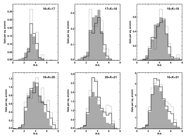
Figure 13: The $R-K$ colour distribution of the galaxies as a function of galaxy $K$-band magnitude. The solid lines represent the distribution combined across all of the 5 fields; the dotted line is the distribution considering only the inner quarter of those fields, corresponding to distances out to about 700 kpc (at $z\sim 1.5$) from the AGN; the shaded region represents the expected field distribution, as derived at $K<20$ by combining the CADIS 16hr field (Thompson et al. 2000) and the K20 survey (Cimatti et al. 2002) and for $20<K<21$ from the compilation of Hall & Green (1998).

Figure 14: The radial distribution of galaxies with $17.5<K<20.7$ and $R-K>4$ in each of the five fields separately, and the average of these. The radius is calculated in kpc at the redshift of each AGN. The error bars represent the Poissonian errors on the galaxy counts in each bin. In each figure the horizontal dotted line represents the expected blank–field distribution.

4.3 Radial distribution of individual fields

Knowing the magnitudes and colours of the galaxies producing the excess counts, it is possible to investigate their radial distribution in each of the galaxy fields separately. Considering only those galaxies with magnitudes $17.5<K<20.7$ and colours $R-K>4$, the radial distribution of the galaxy counts was derived for each field. These results are shown in Figure 14, together with a combined histogram produced by averaging across all five fields. Also included on these plots is the expected number density for blank-field sources of these magnitudes and colours; this was calculated by taking the K20 and CADIS surveys, making the same cuts in colour and magnitude as for the AGN fields, and then convolving the results with the completeness versus magnitude function (Figure 7).

The results from combining the five AGN fields are in agreement with those derived by Hall & Green [1998], namely that a pronounced peak of red galaxies is seen within the inner $\sim$150 kpc, together with a weaker large–scale excess. With the larger field–of–view of the data provided here, it is now possible to quantify the radial extent of this large–scale overdensity: the galaxy counts remain above field expectations out to between 1 and 1.5 Mpc radius.

Comparing the five individual fields in Figure 14, however, it is immediately apparent that this combined result is the average of five fields with very different properties. 0016$-$129 and 2025$-$155 do both show radial distributions similar to the average result, with pronounced peaks in the inner bin followed by weak red galaxy overdensities to $\sim 1$ Mpc. 0000$-$177 has a central pronounced peak of red galaxies, but shows no large–scale excess (indeed quite the opposite); this may be indicative of a compact group of galaxies. 0139$-$273 and 1524$-$136 are both much less centrally concentrated, with smoother central peaks and much more gradual radial declines in red galaxy surface density out to the blank–field expectations at radial distances of between 1 and 1.5 Mpc. There is clearly a large range in the nature, scale and significance of any galaxy overdensities around these AGN.

That the radial distribution of galaxies within these large–scale overdensities is not more sharply peaked should not be surprising. A galaxy cluster with a mass of a few $\times 10^{14}M_{\odot}$ and an initial scale of 3–5 Mpc has an overall density of 1–4 $\times 10^{-25}$ kg m^-3. The time that such a structure will take to separate out from Hubble flow and collapse is $t\sim(3\pi/32G\rho)^{1/2}\sim$ 3–6 Gyr [1999]. The Universe at redshifts $z\sim 1.5$ is about 4.5 Gyr old, and so such structures will still be collapsing into a virialised cluster such as those we see today; the large–scale structures seen around the AGN might even not yet be gravitationally bound.

4.4 Bright red galaxies and sub-structure

At high redshifts most clusters observed to date have several giant galaxies within them, presumably due to merging subclusters. Further, there is some evidence that AGN host galaxies are not always the only bright galaxies in their environment, for example due to sub-cluster mergers or being part of a group falling into a larger structure (e.g. Bremer, Baker & Lehnert 2002; Simpson & Rawlings 2002). Therefore, the fields have been searched for any galaxies other than the AGN that are brighter than $K=18$ and satisfy the colour criteria of the ‘cluster elliptical candidates’ above. The images around these bright red galaxies have then been examined; the majority of these galaxies appear to be fairly isolated, and so are likely to be foreground extremely red objects with redshifts of $z\sim 1$, since such foreground objects will tend to dominate the extremely red galaxy population at brighter magnitudes (e.g. Cimatti et al. 2002). However, in two cases these bright red galaxies have associated fainter red galaxies, and may represent substructures at the AGN redshift.

The first of these cases is in the field of 0000$-$177, where three galaxies with $K=17.41$, $K=17.77$ and $K=17.85$ and colours $R-K>5$ are found close together, along with fainter red galaxies, about an arcminute east of the AGN. Indeed, these galaxies represent the small peak in the red galaxy radial distribution (Figure 14) at 600 to 700 kpc radius around this source. This region of the field is of comparable richness in red galaxies to the regions around the AGN. The second case is a group found around a $K=17.09$ galaxy about 1.5 arcminutes to the south–west of 0016$-$129, partially causing the 800–1000 kpc bump in the radial distribution around that source. This appears even richer than the red galaxy distribution around the radio galaxy itself, which might explain why the value of $N_{\rm 0.5}$ for this source is fairly low even though the number counts are well above the literature average.

It is not clear whether these extra structures are indeed at the same redshifts as the AGN, but if so then this would indicate that any large–scale structure around the AGN is still in the process of building up. It is interesting that this evidence for substructure is found in the two cases with the weakest evidence for red galaxy excesses in the 200–500 kpc radius range.

4.5 The morphology–density relation

In nearby clusters, a well–known morphology–density relation exists [1977, 1980], whereby in regions of high galaxy density, such as the centre of the cluster, higher proportions of early–type galaxies are found. Dressler et al. [1997] investigated the evolution of this morphology–density relation with redshift, out to $z\sim 0.5$, and find that this is still present at these redshifts but only in high-concentration, regular clusters; no correlation between galaxy–type and local galaxy density is found for low-concentration, irregular clusters. They interpret this as meaning that the mechanisms that produce morphological segregation (e.g. dynamical friction, or conversion of late–types into early types by gas stripping and halting star formation) work most rapidly in high mass systems.

The nature of the small–scale galaxy excess around these distant radio sources (and in the two potential substructures) is particularly interesting because, where present, it is comprised almost entirely of red galaxies (cf. Figs 4 to 6). This indicates that morphological segregation may already have taken place in the very inner regions around the AGN, implying that the morphology–density relation is imprinted into cluster centres at a very early epoch.

4.6 Angular cross–correlation analyses

The clustering of galaxies around the radio galaxies can be investigated using the angular cross–correlation function $w(\theta)$, which is defined from the probability ($\delta P$) of finding two sources in areas $\delta\Omega_{1}$ and $\delta\Omega_{2}$ separated by a distance $\theta$: $\delta P=N^{2}[1+w(\theta)]\delta\Omega_{1}\delta\Omega_{2}$, where $N$ is the mean surface density of sources on the sky.

The value of $w(\theta)$ can be evaluated for all galaxy–galaxy pairs, for just AGN–galaxy pairs, or restricting the galaxies included to certain ranges of colours and magnitudes. Here, four different set of galaxy magnitudes and colours were considered: (1) ‘all galaxies’; (2) ‘blue galaxies’; (3) ‘red galaxies’; and (4) ‘cluster elliptical candidates’, which are the subset of the red galaxies that have K magnitudes, $R-K$ and $J-K$ colours in the range that would be expected for old passive cluster galaxies. The exact colour and magnitude definitions of each class of objects, and the number of galaxies contained in that class, are provided in Table 5.

For each of these subsamples of galaxies the value of $w(\theta)$ was estimated for a variety of bins in $\theta$, following the method described by B00, considering both all galaxy–galaxy pairs and only AGN–galaxy pairs. The results obtained over all 5 fields with multi–colour data were averaged to produce overall results, with an estimate of the uncertainty in the value of the combined $w(\theta)$ in each bin provided by the scatter in the values between the different fields. $w(\theta)$ usually shows a power–law form, $w(\theta)=A(\theta/{\rm deg})^{-\delta}$, with a canonical value for the exponent of $\delta=0.8$; this value appears also to be appropriate at high redshifts [1998], and so was adopted here for all fits here. This does not always provide an excellent fit to the data, but the current data do not have sufficient signal–to–noise to warrant an attempt to independently fit this parameter; note that because this parameter is fixed, the formal errors on the cross-correlation amplitudes may be slightly higher than those quoted.

The finite area of the images leads to a small correction, known as the integral constraint ($C$), such that $w(\theta)_{\rm obs}=A[(\theta/{\rm deg})^{-0.8}-C]$. The value of $C$ can be estimated by integrating $w(\theta)$ over the area of each field, and for the current data corresponds to $C_{\rm gg}=16.7$ and $C_{\rm ag}\approx 19.1$ for all galaxy-galaxy pairs and just AGN-galaxy pairs respectively. Using these expressions, the amplitudes of the angular cross–correlation function were derived for both all galaxy–galaxy pairs and just AGN–galaxy pairs for each of the selected colour–magnitude subsamples of galaxies. The cross–correlation functions are displayed in Figure 15, and Table 5 provides the derived cross–correlation amplitudes.

All galaxy–galaxy pairs

AGN–galaxy pairs only

Figure 15: The angular cross–correlation functions for galaxies with a range of magnitudes and colours as defined in Table 5, averaged across the 5 fields. The left–hand plots correspond to all galaxy–galaxy pairs and the right–hand plots consider only AGN–galaxy pairs.

Table 5: Results from the angular cross correlation analyses. For galaxies with a range of magnitudes and colours, the amplitude of the angular cross-correlation function is provided considering both all galaxy–galaxy pairs ($A_{\rm gg}$) and only AGN–galaxy pairs ($A_{\rm ag}$).

Sample	K–mag range	IR col range	IR-opt col range	$N_{\rm gals}$	Angular cross-correlation amplitude
					$A_{\rm gg}$	$A_{\rm ag}$
All galaxies	K$<$20.7	All	All	1739	$0.0005\pm 0.0001$	$0.0065\pm 0.0022$
Blue galaxies	K$<$20.7	J-K$<$1.6	R-J$<$2.5	762	$0.0000\pm 0.0003$	$0.0000\pm 0.0026$
Red galaxies	K$<$20.7	J-K$>$1.4	R-J$>$2.0	868	$0.0020\pm 0.0002$	$0.0166\pm 0.0041$
Cluster ellips?	17.0$<$K$<$20.5	1.6$<$J-K$<$2.2	3.0$<$R-J$<$4.5	252	$0.0042\pm 0.0004$	$0.0307\pm 0.0052$

The angular cross–correlation amplitude of ‘all galaxies’ in these fields is within the range of the values recently derived to $K=20.75$ for ‘blank–fields’ (e.g. Carlberg et al. 1997; Roche et al. 2002; Daddi et al. 2000a). However, comparing the values of $A_{\rm gg}$ and $A_{\rm ag}$ in Table 5 shows that the galaxies are much more highly clustered around the AGN than around other galaxies in general, indicating that a significant proportion of the galaxies are connected with the AGN. Evidence for such clustering around the AGN is particularly apparent when comparing the results for galaxies of different colours. The blue galaxies show no evidence for clustering, not even around the AGN, whilst red galaxies are known to be more highly clustered (e.g. Roche et al. 1996, Shepherd et al. 2001 and references therein) and this is reflected in the value of $A_{\rm gg}$ derived for this class; their higher value of $A_{\rm ag}$ shows that these are preferentially clustered around the AGN. The ‘cluster elliptical candidates’ have even larger values of $A_{\rm gg}$ and $A_{\rm ag}$, suggesting that this selection criteria picks out a highly clustered class of object, many of which are indeed likely to be old passive cluster ellipticals. It should be noted that this clustering signal is dominated by the points at small radii, $\theta\mathrel{\hbox to0.0pt{\lower 3.0pt\hbox{$\mathchar 536\relax$}\hss}\raise 2.0pt\hbox{$\mathchar 316\relax$}}10$ arcsec, corresponding to the excess in the upper left panel of Figure 12; however, even if the inner two bins of the cross–correlation analysis are ignored, the clustering amplitude around the AGN is still higher than that of the field in general, indicating that it is not only these nearby galaxies which produce the clustering signal.

If a population of $N_{\rm c}$ cluster galaxies, with a high intrinsic angular cross–correlation amplitude ($A_{\rm c}$), is observed together with a sample of $N_{\rm i}$ foreground or background interloper galaxies with zero clustering amplitude, then the resultant combined sample will have an observed cross–correlation amplitude of $\approx\frac{N_{\rm c}}{N_{\rm c}+N_{\rm i}}A_{\rm c}$. In other words, the observed amplitude will be the amplitude that would be found for the cluster galaxies alone, scaled down by the proportion of the total sample that are cluster galaxies. This situation is a good approximation to those of the ‘red galaxy’ and ‘cluster elliptical candidate’ samples, since the observed value of $A_{\rm gg}$ for these samples are almost an order of magnitude below those of $A_{\rm ag}$. Comparing the values of $A_{\rm ag}$ then indicates that the colour definition for the ‘cluster elliptical candidate’ sample approximately halves the fraction of interlopers relative to the red galaxies.

If the results from the number count analysis are taken at face value, then there are about 270 clusters galaxies across the five fields studied in the cross–correlation analysis (290 excess galaxies determined in Section 4.1, of which 20 are from the 2128$-$208 field, not considered here); using this, an estimate can be made for the number of cluster galaxies in each of the colour–selected samples. Assuming that about 80% of the cluster galaxies are ‘red’ (from Figure 13) then within the ‘red galaxy’ sample there are about 220 cluster galaxies, which corresponds to about 25% of the overall ‘red galaxy’ sample (see Table 5). This would suggest that about 40% of the ‘cluster elliptical candidate’ sample, that is $\sim$100 galaxies, are indeed cluster galaxies. If these results are correct, the $\sim$100 early–type cluster galaxies at redshifts $z\sim 1.6$ would provide a substantial sample for cluster galaxy evolution studies.

As has been described by many authors (e.g. Longair & Seldner 1979, Prestage and Peacock 1988), if the form of the galaxy luminosity function at the redshift of the AGN is assumed, it is possible to convert the amplitude of the angular cross–correlation function for galaxies around the AGN into a spatial cross–correlation amplitude, $B_{\rm ag}$, derived from the spatial cross–correlation function $\xi(r)=B_{\rm ag}\left(\frac{r}{{\rm Mpc}}\right)^{-\gamma}$. Following the method of B00, the value of $A_{\rm ag}=0.0061\pm 0.0022$ for the ‘all galaxies’ sample corresponds to a spatial cross–correlation amplitude of $B_{\rm ag}=660\pm 240$. This amplitude is comparable to the value of $B_{\rm ag}=510\pm 120$ derived by B00 around 3CR radio galaxies with redshifts $z\sim 1$. These values can be interpreted physically by comparing with the equivalent values ($B_{\rm cg}$) for Abell clusters calculated between the central galaxy and the surrounding galaxies; these have been derived by several authors and average to $B_{\rm cg}\approx 350$ for Abell class 0 and $B_{\rm cg}\approx 710$ for Abell class 1 [1988, 1991, 1994, 1999]. The environments surrounding these $z\sim 1.6$ AGN seem to be, on average, comparable to those of local clusters of richness between Abell classes 0 and 1.

5 Environmental variations compared with radio source properties

The results have clearly shown that the environments of these high redshift AGN are heterogeneous, with considerable variation in both the amplitude and the physical extent of any galaxy excess. In this section the variations in the galaxy overdensities are compared with the other properties of the radio source, to see if there are any indications of why the environments differ so much. The properties of the radio sources studied are provided in Table 6.

The first thing to note is that all of these radio sources have essentially the same redshifts and radio powers, and so the variations are not generally correlated with either of these properties. Equally, all 6 studied sources are steep–spectrum radio sources according to the standard definition of $\alpha>0.5$ (where $\alpha$ is defined as $S_{\nu}\propto\nu^{-\alpha}$), although 1524$-$136 has a spectral index close to this cut–off; the weaker small–scale excess of this source could conceivable be related to this in some way. No fundamental difference is seen between the quasar and radio galaxy populations, and nor is any correlation with the size of the radio source seen for any of the extended radio sources.

The only issue which this comparison does bring to light is that the one source for which no overdensity is seen on either large or small scales, 2128$-$208, is an unresolved radio source; this could potentially explain this result. Extended radio sources must have been fueled continuously for timescales of at least $10^{6}$ years, and possibly up to $10^{8}$ years, which requires a plentiful and steady supply of fueling gas, as well as a relatively dense surrounding medium to confine the expanding radio lobes. Perhaps at high redshifts these conditions are only satisfied for galaxies within larger–scale structures. On the other hand, compact radio sources are relatively young, $\mathrel{\hbox to0.0pt{\lower 3.0pt\hbox{$\mathchar 536\relax$}\hss}\raise 2.0pt\hbox{$\mathchar 316\relax$}}10^{5}$ years old (e.g. Owsianik and Conway 1998), and it has been suggested that some proportion of these may fizzle out before evolving into larger radio sources (e.g. Alexander 2000). The reduced gas supply required for these short–lived compact sources may then be available to galaxies in any environment, and could explain the lack of any overdensities around 2128$-$208.

This situation has been modelled by Kauffmann & Haehnelt [2002] who have investigated the quasar–galaxy cross–correlation function around quasars at different redshifts within hierarchical clustering models of galaxy formation. In their model they assume that quasars are triggered by galaxy mergers, with some percentage of the gas brought in by the merger then fuelling the black hole. They show that the cross–correlation function around the quasars is significantly higher for quasars with long lifetimes than for short–lived sources, in agreement with the discussion above. This difference is most pronounced for the most powerful AGN, such as those studied here.

An alternative may be that this is a lower power radio source with its flux density Doppler boosted by beaming; in this case a correlation between radio power and environmental density would explain the result. However, a beaming scenario is considered unlikely due to the steep spectral index of the source.

Table 6: Properties of the 6 radio sources studied.

Source	z	$S_{\rm 408}$	$\alpha_{1400}^{408}$	$P_{\rm 408}$	D	Type	Excess on scale∗
		[Jy]		[$10^{27}$ W Hz-1]	[′′]		$\mathrel{\hbox to0.0pt{\lower 3.0pt\hbox{$\mathchar 536\relax$}\hss}\raise 2.0pt\hbox{$\mathchar 316\relax$}}$150 kpc	$\sim$1 Mpc
MRC 0000-177	1.47	6.51	0.80	85.4	2.7	Q	Y	N
MRC 0016-129	1.59	6.87	0.95	125.4	3.5	RG	Y	y
MRC 0139-273	1.44	5.04	0.95	72.2	12	RG	y	Y
MRC 1524-136	1.69	6.11	0.61	92.5	0.4	Q	y?	Y
MRC 2025-155	1.50	5.41	1.05	93.9	15	Q	Y	y
MRC 2128-208	1.62	6.15	0.88	110.1	$<1$	Q	N	N

^∗ ’Y’ = strong-excess; ’y’ = weak excess; N = no significant excess.

6 Discussion and Conclusions

The results of this work can be summarised as follows.

• On average, a significant overdensity of K–band selected galaxies with $17.5<K<20.5$ is found across the AGN fields.

• These excess counts are predominantly associated with galaxies with magnitudes $K\mathrel{\hbox to0.0pt{\lower 3.0pt\hbox{$\mathchar 536\relax$}\hss}\raise 2.0pt\hbox{$\mathchar 318\relax$}}17.5$ and colours $R-K\mathrel{\hbox to0.0pt{\lower 3.0pt\hbox{$\mathchar 536\relax$}\hss}\raise 2.0pt\hbox{$\mathchar 318\relax$}}4$, which are (although not uniquely) exactly those expected for old passive cluster galaxies at redshifts $z\sim 1.6$.

• These galaxies are found on two different spatial scales around the AGN: pronounced concentrations of galaxies at radial distances $\mathrel{\hbox to0.0pt{\lower 3.0pt\hbox{$\mathchar 536\relax$}\hss}\raise 2.0pt\hbox{$\mathchar 316\relax$}}150$ kpc, and weaker large–scale overdensities extending out to between 1 and 1.5 Mpc.

• The presence or absence of galaxy excesses on these two scales differs greatly from AGN field to AGN field. All of the extended radio sources show overdensities on some scale: two show overdensities on both scales, two predominantly on large scales and one only on small scales. The one field which shows little evidence for a galaxy excess on any scale is associated with an unresolved radio source.

• Where overdensities are present on $\mathrel{\hbox to0.0pt{\lower 3.0pt\hbox{$\mathchar 536\relax$}\hss}\raise 2.0pt\hbox{$\mathchar 316\relax$}}150$ kpc scales, these are composed almost entirely of red galaxies. This suggests that the morphology–density relation is imprinted into the centres of clusters at a very early stage of cluster formation.

• The amplitude of the angular cross–correlation function around the AGN is a strong function of galaxy colour. The selection of only galaxies with magnitudes and colours consistent with being old passive elliptical galaxies at the AGN redshifts maximises this amplitude, indicating that old ellipticals do indeed exist in these environments.

• The spatial cross–correlation amplitude for all galaxies around the AGN is similar to that around the 3CR radio galaxies at redshifts $z\sim 1$; both are consistent with having the same richness as local Abell clusters of richness class 0 to 1.

It is interesting to consider what these results imply for the nature of the AGN at these redshifts, and also for cluster evolution.

Powerful radio galaxies are known to be hosted by giant elliptical galaxies at all redshifts $z\mathrel{\hbox to0.0pt{\lower 3.0pt\hbox{$\mathchar 536\relax$}\hss}\raise 2.0pt\hbox{$\mathchar 316\relax$}}1.3$ (e.g. Best et al. 1998, McLure & Dunlop 2000), and even out to redshifts $z<2.4$ a significant proportion still have radial profiles well–matched by de Vaucouleurs’ law [2001]. Little difference is found between the host galaxies of radio galaxies and radio–loud quasars at these redshifts [2001], which suggests that the hosts of all of the $z\sim 1.5$ AGN studied here are likely to be giant elliptical galaxies.

The variety of different environments found for these AGN may simply reflect this fact: that the primary requirement for forming a powerful radio–loud AGN is a giant elliptical galaxy host. Such galaxies can be found in a range of environments from galaxy clusters, through groups of galaxies, to relatively isolated environments, but are generally only formed by redshifts $z\sim 1.6$ when they are found at the highest peaks of the primordial density perturbations, within larger–scale structures. This explains the high average richness, but still significant variation, of the large–scale galactic environments around these AGN.

To understand the pronounced smaller scale galaxy overdensity, the key question is whether these central galaxies represent a stable virialised structure, or whether they are still infalling and will merge with the central radio galaxy. If these are already virialised then the small scale galaxy overdensity is clearly related to the larger–scale structure, and indicates that at least some of the AGN lie at a special location in their environments: at the centres of their clusters or groups. This again is not too surprising: the kinetic energy of the relativistic radio jets of these AGN corresponds to the Eddington luminosity of a black hole with $M\sim 10^{9}\,M_{\odot}$ [1991], and so even assuming that these sources are fueled close to the Eddington limit they must be powered by very massive central engines and the radio lobes must be confined by dense gas. It is not unreasonable to expect these most powerful radio sources to be found within the most massive elliptical galaxies, at the centre of the cluster or group of galaxies.

In this interpretation, the four different scenarios of the presence or absence of galaxy overdensities on small and large scales correspond to four different possible locations of the AGN host galaxy: it may be a central cluster galaxy in cluster with a virialised core (excesses on both scales), an off–centre giant elliptical in a cluster, or the central galaxy in a cluster at an early stage of formation (only large–scale overdensity), the central galaxy of a compact group (only small–scale excess), or an isolated giant elliptical (no excess on any scale). With respect to this model, it is interesting that all of the extended radio sources lie in group or cluster environments.

Alternatively, if the galaxies producing the small–scale excess are not yet virialised, then they may instead be related to a hierarchical build up of the central AGN host galaxy. Pentericci et al. [2001] found that the optical characteristic sizes of powerful radio galaxies are typically a factor of two smaller at $z\sim 2$ than those at $z\sim 1$. Since the galaxy luminosity and the characteristic size of ellipticals are related by $L_{\rm int}\propto r_{\rm e}^{0.7}$ [1977], this means that the radio galaxies must grow in mass by about a factor of two over this redshift interval, a large part of which may be due to mergers with companion galaxies. If the 150 kpc scale galaxy excess has a velocity dispersion $\sigma\sim 500$ km s^-1, then the galaxy crossing time for this structure is $\sim 0.3$ Gyr. A galaxy merger timescale of a few crossing times is therefore comparable to the interval of cosmic time between redshifts $z\sim 2$ and $z\sim 1$, and some of the small–scale excesses of galaxies may be destined to merge with the AGN host galaxy soon.

Whichever of these interpretations for the small–scale galaxy excess around the AGN is correct (and undoubtedly a combination of both effects is occurring), the Mpc–scale galaxy overdensities appear be associated with (proto?) cluster environments. The wealth of galaxies with magnitudes and colours consistent with being old elliptical galaxies at $z\sim 1.6$ indicate that the epoch of elliptical galaxy formation must be earlier than this redshift; the colours of these objects further suggest that the bulk of their stellar populations must have formed at redshifts $z\mathrel{\hbox to0.0pt{\lower 3.0pt\hbox{$\mathchar 536\relax$}\hss}\raise 2.0pt\hbox{$\mathchar 318\relax$}}5$ (this will be discussed further in Best et al. in preparation). By using these radio–loud AGN as signposts, it is therefore possible to define significant samples of $z\sim 1.6$ cluster early–type galaxies with which to extend studies of galaxy evolution back to earlier cosmic epochs.

Finally, it is interesting to compare the comoving number density of these powerful radio sources with that of nearby rich clusters. According to the pure luminosity evolution model for steep–spectrum radio sources of Dunlop and Peacock [1990], at redshifts $z=1$ to 2, there are about $10^{-7}$ radio sources per comoving Mpc³ within the upper decade of radio luminosities containing the sources studied here. By comparison, the comoving number density of nearby clusters of Abell richness class 0 or greater is $\sim 4\times 10^{-6}$ Mpc^-3, and for Abell class 1 and richer it is $\sim 1.7\times 10^{-6}$ Mpc^-3 (e.g. Bahcall & Soniera 1983; converted to the cosmology adopted in this paper; cf. West 1994). However, radio sources only live for between $10^{7}$ and $10^{8}$ years (e.g. Kaiser et al. 1997), and so the observed number density of powerful radio sources underestimates the number density of environments which will contain a powerful radio source at some point between redshifts 2 and 1 by a factor $\sim 50$ ($=$ cosmic time between redshift 2 and 1 divided by the lifetime of a typical radio source). Therefore, the comoving number density of environments which will contain a powerful radio source between redshifts 2 and 1 is comparable to the comoving number density of nearby Abell clusters of richness class 0 or greater. This may simply be an interesting coincidence, or alternatively may imply that the onset of a powerful radio source is a key stage in the formation of a rich cluster.

References

- [1958] Abell G. O., 1958, ApJ Supp., 3, 211
- [2000] Alexander P., 2000, MNRAS, 319, 8
- [1994] Andersen V., Owen F. N., 1994, AJ, 108, 361
- [1998] Bahcall N. A., Fan X., 1998, ApJ, 504, 1
- [1983] Bahcall N. A., Soneira R. M., 1983, ApJ, 270, 20
- [1998] Bershady M. A., Lowenthal J. D., Koo D. C., 1998, ApJ, 505, 50
- [1996] Bertin E., Arnouts S., 1996, A&A Supp., 117, 393
- [2000] Best P. N., 2000, MNRAS, 317, 720 [B00]
- [1998] Best P. N., Longair M. S., Röttgering H. J. A., 1998, MNRAS, 295, 549
- [1999] Best P. N., Röttgering H. J. A., Lehnert M. D., 1999, MNRAS, 310, 223
- [2000] Best P. N., Röttgering H. J. A., Lehnert M. D., 2000, MNRAS, 315, 21
- [2002] Bremer M. N., Baker J. C., Lehnert M. D., 2002, MNRAS, 337, 470
- [1997] Carlberg R. G., Pritchet C. J., Infante L., 1997, ApJ, 435, 540
- [1987] Chambers K. C., Miley G. K., van Breugel W. J. M., 1987, Nat, 329, 604
- [2002] Cimatti A., Daddi E., Mignoli M., Pozzetti L., Renzini A., Zamorani G., Broadhurst T., Fontana A., Saracco P., Poli F., Cristiani S., D’Odorico S., Giallongo E., Gilmozzi R., Menci N., 2002, A&A, 381, L68
- [1996] Crawford C. S., Fabian A. C., 1996, MNRAS, 282, 1483
- [2000a] Daddi E., Cimatti A., Pozzetti L., Hoekstra H., Röttgering H. J. A., Renzini A., Zamorani G., Mannucci F., 2000a, A&A, 361, 535
- [2000b] Daddi E., Cimatti A., Renzini A., 2000b, A&A, 362, L45
- [2002] De Breuck C., van Breugel W., Stanford S. A., Röttgering H., Miley G., Stern D., 2002, AJ, 123, 637
- [1997] Delthorn J.-M., Le Fèvre O., Crampton D., Dickinson M., 1997, ApJ, 483, L21
- [1997] Dickinson M., 1997, in Tanvir N. R., Aragón-Salamanca A., Wall J. V., eds, HST and the high redshift Universe. Singapore: World Scientific, p. 207
- [1995] Djorgovski S., Soifer B. T., Pahre M. A., Larkin J. E., Smith J. D., Neugebauer G., Smail I., Matthews K., Hogg D. W., Blandford R. D., Cohen J., Harrison W., Nelson J., 1995, ApJ, 438, L13
- [1980] Dressler A., 1980, ApJ, 236, 351
- [1997] Dressler A., Oemler A., Couch W. J., Smail I., Ellis R. S., Barger A., Butcher H., Poggianti B. M., Sharples R. M., 1997, ApJ, 490, 577
- [1990] Dunlop J. S., Peacock J., 1990, MNRAS, 247, 19
- [1996] Dunlop J. S., Peacock J., Spinrad H., Dey A., Jimenez R., Stern D., Windhorst R., 1996, Nat, 381, 581
- [2001] Fabian A. C., Crawford C. S., Ettori S., Sanders J. S., 2001, MNRAS, 322, L11
- [1993] Gardner J. P., Cowie L. L., Wainscoat R. J., 1993, ApJ, 415, L9
- [1998] Giavalisco M., Steidel C. C., Adelberger K. L., Dickinson M. E., Pettini M., Kellogg M., 1998, ApJ, 503, 543
- [1998] Hall P. B., Green R. F., 1998, ApJ, 507, 558
- [2001] Hall P. B., Sawicki M., Martini P., Finn R., Pritchet C. J., Osmer P. S., McCarthy D., Evans A. S., Lin H., Hartwick F. D. A., 2001, AJ, 121, 1840
- [1991] Hill G. J., Lilly S. J., 1991, ApJ, 367, 1
- [1997] Kaiser C. R., Dennett-Thorpe J., Alexander P., 1997, MNRAS, 292, 723
- [2002] Kauffmann G., Haehnelt M., 2002, MNRAS, 332, 529
- [1977] Kormendy J., 1977, ApJ, 217, 406
- [1980] Kron R. G., 1980, ApJ Supp., 43, 305
- [2001] Kukula M. J., Dunlop J. S., McLure R. J., Miller L., Percival W. J., Baum S. A., O’Dea C. P., 2001, MNRAS, 326, 1533
- [2000] Kurk J. D., Röttgering H. J. A., Pentericci L., Miley G. K., 2000, A&A, 358, L1
- [1981] Large M. I., Mills B. Y., Little A. G., Crawford D. F., Sutton J. M., 1981, MNRAS, 194, 693
- [1992] Lehnert M. D., Heckman T. M., Chambers K. C., Miley G. K., 1992, ApJ, 393, 68
- [1984] Lilly S. J., Longair M. S., 1984, MNRAS, 211, 833
- [1979] Longair M. S., Seldner M., 1979, MNRAS, 189, 433
- [1995] McCarthy P. J., Spinrad H., van Breugel W. J. M., 1995, ApJ Supp., 99, 27
- [1987] McCarthy P. J., van Breugel W. J. M., Spinrad H., Djorgovski S., 1987, ApJ, 321, L29
- [1995] Mcleod B. A., Bernstein G. M., Rieke M. J., Tollestrup E. V., Fazio G. G., 1995, ApJ Supp., 96, 117
- [2000] McLure R. J., Dunlop J. S., 2000, MNRAS, 317, 249
- [1977] Melnick J., Sargent W. L. W., 1977, ApJ, 215, 401
- [198] Minezaki T., Kobayashi Y., Yoshii Y., Peterson B. A., 198, ApJ, 494, 111
- [1998] Monet D., Bird A., Canzian B., Dahn C., Guetter H., Harris H., Henden A., Levine S., Luginbuhl C., Monet A. K. B., Rhodes A., Riepe B., Sell S., Stone R., Vrba F., Walker R., 1998, The USNO-A2.0 Catalogue. U.S. Naval Observatory, Washington DC
- [1997] Moustakas L. A., Davis M., Graham J. R., Silk J., Peterson B. A., Yoshii Y. L. M., Coles P., Lucchin F., Matarrese S., 1997, ApJ, 475, 445
- [1998] Owsianik I., Conway J. E., 1998, A&A, 69, 337
- [1999] Peacock J. A., 1999, Cosmological Physics. Cambridge University Press
- [2001] Pentericci L., McCarthy P. J., Röttgering H. J. A., Miley G. K., van Breugel W. J. M., Fosbury R., 2001, ApJ Supp., 135, 63
- [1988] Prestage R. M., Peacock J. A., 1988, MNRAS, 230, 131
- [1991] Rawlings S., Saunders R., 1991, Nat, 349, 138
- [2002] Roche N., Almaini O., Dunlop J. S., Ivison R. J., Willott C. J., 2002, MNRAS, submitted; astro-ph/0205259
- [1996] Roche N., Shanks T., Metcalfe N., Fong R., 1996, MNRAS, 280, 397
- [1999] Saracco P., D’Odorico S., Moorwood A., Buzzoni A., Cuby J.-G., Lidman C., 1999, A&A, 349, 751
- [2001] Shepherd C. W., Carlberg R. G., Yee H. K. C., Morris S. L., Lin H., Sawicki M., Hall P. B., Patton D. R., 2001, ApJ, 560, 72
- [2002] Simpson C., Rawlings S., 2002, MNRAS, 334, 511
- [1997] Spinrad H., Dey A., Stern D., Dunlop J., Peacock J., Jimenez R., Windhorst R., 1997, ApJ, 484, 581
- [1998] Stanford S. A., Eisenhardt P. R., Dickinson M., 1998, ApJ, 492, 461
- [2002] Stanford S. A., Holden B., Rosati P., Eisenhardt P. R., Stern D., Squires G., Spinrad H., 2002, AJ, 123, 619
- [1998] Szokoly G. P., Subbarao M. U., Connolly A. J., Mobasher B., 1998, ApJ, 492, 452
- [1999] Thompson D., Beckwith S. V. W., Fockenbrock R., Fried J., Hippelein H., Huang J.-S., von Kuhlmann B., Leinert C., Meisenheimer K., Phleps S., Röser H.-J., Thommes E., Wolf C., 1999, ApJ, 523, 100
- [2001] Totani T., Yoshii Y., Maihara T., Iwamuro F., Motohara K., 2001, ApJ in press; astro-ph/0106323
- [2000] Väisänen P., Tollestrup E. V., Willner S. P., Cohen M., 2000, ApJ, 540, 593
- [1999] van Breugel W. J. M., De Breuck C., Stanford S. A., Stern D., Röttgering H. J. A., Miley G. K., 1999, ApJ, 518, L61
- [1998] van Dokkum P. G., Franx M., Kelson D. D., Illingworth G. D., 1998, ApJ, 504, L17
- [2002] Venemans B. P., Kurk J. D., Miley G. K., Röttgering H. J. A., van Breugel W., Carilli C. L., De Breuck C., Ford H., Heckman T., McCarthy P., Pentericci L., 2002, ApJ, 569, L11
- [1994] West M. J., 1994, MNRAS, 268, 79
- [2000] Wold M., Lacy M., Lilje P. B., Serjeant S., 2000, MNRAS, 316, 267
- [1989] Yates M. G., Miller L., Peacock J. A., 1989, MNRAS, 240, 129
- [1999] Yee H. K. C., López–Cruz O., 1999, AJ, 117, 1985