Three-Point Correlations in Weak Lensing Surveys: Model Predictions and Applications

Abstract

We use the halo model of clustering to compute two- and three-point correlation functions for weak lensing, and apply them in a new statistical technique to measure properties of massive halos. We present analytical results on the eight shear three-point correlation functions constructed using combination of the two shear components at each vertex of a triangle. We compare the amplitude and configuration dependence of the functions with ray-tracing simulations and find excellent agreement for different scales and models. These results are promising, since shear statistics are easier to measure than the convergence. In addition, the symmetry properties of the shear three-point functions provide a new and precise way of disentangling the lensing $E$-mode from the $B$-mode due to possible systematic errors.

We develop an approach based on correlation functions to measure the properties of galaxy-group and cluster halos from lensing surveys. Shear correlations on small scales arise from the lensing matter within halos of mass $M\lower 2.15277pt\hbox{$\;\buildrel>\over{\sim}\;$}10^{13}M_{\odot}$. Thus, the measurement of two- and three-point correlations can be used to extract information on halo density profiles, primarily the inner slope and halo concentration. We demonstrate the feasibility of such an analysis for forthcoming surveys. We include covariances in the correlation functions due to sample variance and intrinsic ellipticity noise to show that 10% accuracy on profile parameters is achievable with surveys like the CFHT Legacy survey, and significantly better with future surveys. Our statistical approach is complementary to the standard approach of identifying individual objects in survey data and measuring their properties. It can be extended to perform a combined analysis of the large-scale, perturbative regime down to small, sub-arcminute scales, to obtain consistent measurements of cosmological parameters and halo properties.

1 Introduction

The gravitational lensing of distant galaxy images due to large-scale structure, known as cosmic shear, has been well established as a cosmological probe (e.g, Mellier 1999, Bartelmann & Schneider 2001 and Wittman 2002 for reviews). Many independent groups have reported significant detections of two-point shear correlations, providing constraints on the mass density of the universe ($\Omega_{\rm m0}$) and the mass power spectrum amplitude ($\sigma_{8}$) (e.g., Van Waerbeke et al. 2001b; Bacon et al. 2002; Refregier, Rhodes & Groth 2002; Hoekstra et al. 2002; Brown et al. 2002; Hamana et al. 2002; Jarvis et al. 2003). Non-linear gravitational clustering substantially enhances the cosmic shear signal on angular scales $\lower 2.15277pt\hbox{$\;\buildrel<\over{\sim}\;$}10^{\prime}$ (Jain & Seljak 1997). An accurate description of non-linear effects on shear correlations is important to interpret the measurements.

The most effective way of studying non-linear structure formation has been $N$-body simulations, which are accurate on scales larger than the numerical resolution limit, since the relevant physics is only gravity on scales of interest. However, current survey data require accurate models of large-scale structure over a huge dynamic range of length scales. A simulation needs to sample cosmological scale $(\sim 100$Mpc) in order to have a fair sample. On the other hand, lensing statistics at relevant angular scales are affected by highly non-linear structures, dark matter halos with a size $\;\buildrel<\over{\sim}\;$Mpc, and structure that needs to be resolved down to scales approaching $0.01$Mpc. The required dynamic range is prohibitive for current computational resources. In addition, to perform multiple evaluations in model parameter space requires thousands of simulations runs, which is also prohibitive. While some numerical short-cuts can be used to get around these constraints, having an accurate analytic model would be a valuable complementary, and sometimes essential, tool. It could also provide physical insights into the complex non-linear phenomena involved in gravitational clustering.

The dark matter halo model of clustering fulfills such a niche. The method was first constructed in real space to understand the correlation functions of the galaxy distribution in terms of halos (Neyman & Scott 1952; Peebles 1974; McClelland & Silk 1977; Scherrer & Bertschinger 1991; Sheth & Jain 1997; Yano & Gouda 1999; Ma & Fry 2000a,b; Sheth et al. 2001; Berlind & Weinberg 2002; Takada & Jain 2003b, hereafter TJ03b). The model was also formulated in Fourier space, since this leads to simpler expressions for the Fourier-transformed counterparts of the higher-order moments (Seljak 2000; Peacock & Smith 2000; Ma & Fry 2000c; Scoccimarro et al. 2001; Cooray & Hu 2001a,b; Takada & Jain 2002 hereafter TJ02; also see Cooray & Sheth 2002 for a review). Given the model ingredients: the halo density profile, mass function and bias, each of which has been well investigated in the literature, the halo model can be used to compute the statistics of cosmic fields. There are several advantages in using the halo model. First, it allows us to easily implement multiple model predictions in parameter space. Second, the measured signals are explicitly understood in terms of the halo model ingredients. This will be relevant for the comparison with other observations such as the $X$-ray or the Sunyaev-Zel’dovich (SZ) effect for clusters of galaxies. Third, the model accuracy can be easily refined by incorporating results from $N$-body simulations with higher resolution. Interestingly, so far the halo model has led to consistent predictions to interpret observational results of galaxy clustering as well as reproduce simulation results (e.g., Seljak 2000; Ma & Fry 2000c; Scoccimarro et al. 2001; TJ02; Guzik & Seljak 2002; Sheth et 2001; Takada & Jain 2003a hereafter TJ03a; TJ03b; Zehavi et al. 2003).

Recently, we have extended the halo approach to analytically compute the real-space three-point correlation functions (3PCF) of the mass, galaxies and weak lensing fields with reasonable computational expense (TJ03b). The 3PCF is the lowest-order statistical quantity to probe non-Gaussianity, generated by non-linear structure formation from primordial Gaussian fluctuations. It also allows one to explore the shapes of clustered mass distributions via its configuration dependence, which is not contained in the two-point correlation function (2PCF). Hence, measurements of the 3PCF can provide additional cosmological information. Our recent work described above and this paper provide the methods and formalism to compute the real space 3PCF. On large scales, the real space 3PCF provides no advantage over the well studied bispectrum. On small scales, however, it is easier to measure the 3PCF in real space because the bispectrum requires taking the Fourier transform of survey data, which typically involves dealing with the complex survey geometry (e.g. in lensing surveys there are several areas that are masked out due to bright stars, and thus the transform is likely noisy). In addition, the different wavenumber modes are highly correlated with each other on small scales, and thus one merit of working in Fourier space is lost (in contrast to the CMB, where nonlinearties are minimal on scales of interest). Indeed so far most measurements of the 2PCF have also been in real-space for cosmic shear (though Pen, Van Waerbeke & Mellier 2002; Brown et al. 2002; Pen et al. 2003 have estimated the shear power spectrum as well).

In lensing surveys, the 3PCF of the shear is easier to measure than the 3PCF of the convergence field which requires a non-local reconstruction from the data (Bernardeau, Van Waerbeke & Mellier 2003). An exciting recent development has been the detection of statistical measures based on the shear 3PCF from the Virmos-Descart Survey (Bernardeau, Mellier & Van Waerbeke 2002; Pen et al. 2003). Theoretical study of the shear 3PCF has just begun: Schneider & Lombardi (2003, hereafter SL03) and Zaldarriaga & Scoccimarro (2003, hereafter ZS03) analyzed how to construct the eight shear 3PCFs from combinations of the $+/\times$ shear components at each vertex of a given triangle. Using the ray-tracing simulations, in TJ03a we verified that the eight shear 3PCFs display characteristic configuration dependences, and pointed out that the characteristics can be used to separate the lensing $E$-mode from the measured signals that are generally contaminated by the $B$-mode due to systematic errors and other effects.

The purpose of this paper is to develop an accurate, analytic model to predict the 3PCFs of the shear field, extending the halo model for the convergence field (TJ03b). We will carefully examine the accuracy of the model predictions by comparing with ray-tracing simulations. In particular, we will focus on whether or not the halo model can reproduce the complex configuration dependences seen in the simulations, since the halo model relies on simplified assumptions of spherical halos.

We develop a new application of higher order shear correlations to measure the properties of massive halos. These are relevant for upcoming surveys such as the CFHT Legacy Survey and the Deep Lens Survey and proposed projects such as DML/LSST, Pan-STARRS and SNAP. These surveys promise to measure $n$-point correlation functions of the cosmic shear fields even on sub-arcminutes scales with high significance. Therefore, with the halo model, these small-scale signals can be used to probe properties of the halo density profile such as its inner slope and concentration. We will work with a generalized universal profile for halos (Navarro, Frenk & White 1996; 1997, hereafter NFW). These properties remain uncertain theoretically as well as observationally. To implement this approach, we will develop a method to compute the covariance for the 2PCF and 3PCF measurements, extending the method of Schneider et al. (2002b). We will estimate the accuracy with which forthcoming surveys can constrain halo profile parameters from combined measurements of the 2PCF and 3PCF.

The plan of this paper is as follows. In §2, we develop the real-space halo approach for computing the two- and three-point correlation functions of the lensing convergence and shear fields. In §3, we summarize the triangle configuration dependences of the shear 3PCFs. In §4, we compare the halo model predictions with ray-tracing simulation results. Then, in §5, we show how measurements of the 2PCF and 3PCF on sub-arcminute scales are feasible for ongoing and future lensing surveys, taking into account statistical sources of error. We then address how these small-scale measurements can be used to constrain halo profile properties. §6 is devoted to a summary and discussion. We will consider mainly two cosmological models. One is the $\Lambda$CDM model with $\Omega_{m0}=0.3$, $\Omega_{\lambda 0}=0.7$, $\Omega_{\rm b0}$, $h=0.7$ and $\sigma_{8}=0.9$. The other is the SCDM model with $\Omega_{m0}=1.0$, $h=0.5$ and $\sigma_{8}=0.6$. Here $\Omega_{\rm m0}$, $\Omega_{b0}$ and $\Omega_{\lambda 0}$ are the present-day density parameters of matter, baryons and the cosmological constant, $h$ is the Hubble parameter, and $\sigma_{8}$ is the rms mass fluctuation in a sphere of radius $8h^{-1}$Mpc.

2 Formalism: Real-space Halo Approach to Cosmic shear statistics

In this section we develop an analytic method for calculating the 3PCFs of shear fields by extending the real-space halo approach developed in TJ03b.

2.1 Convergence and shear fields

Weak gravitational lensing can be separated into two effects: magnification (described by the convergence) and shear (e.g., Bartelmann & Schneider 2001).

The lensing convergence field is a scalar quantity and simply expressed as a weighted projection of the density fluctuation field between source galaxy and observer:

$$\kappa(\mbox{{\it\boldmath$\theta$}})=\frac{1}{2}\nabla^{2}\Psi(\mbox{{\it\boldmath$\theta$}})=\int_{0}^{\chi_{H}}\!\!d\chi W(\chi)\delta[\chi,d_{A}(\chi)\mbox{{\it\boldmath$\theta$}}],$$ (1)

where we have introduced the two-dimensional lensing potential $\Psi$, the Laplacian operator $\nabla^{2}$ defined as $\nabla^{2}\equiv\partial^{2}/\partial\theta_{i}\partial\theta_{i}$, $\chi$ is the comoving distance, and $\chi_{H}$ is the distance to the horizon. Note that $\chi$ is related to redshift $z$ via the relation $d\chi=dz/H(z)$, where $H(z)$ is the Hubble parameter at epoch $z$. Following the early work of Blandford et al. (1991), Miralda-Escude (1991) and Kaiser (1992), we used two key simplifications to derive the equation above; the flat-sky approximation, which is valid on angular scales of interest, and the Born approximation, where the convergence field is computed along the unperturbed path. Using ray-tracing simulations, Jain et al. (2000) showed that the Born approximation is an excellent approximation for the two-point statistics. We will assume that it also holds for the higher-order statistics we are interested in. The function $W$ is the lensing projection defined by

$$W(\chi)=\frac{3}{2}\Omega_{m0}H_{0}^{2}a^{-1}(\chi)d_{A}(\chi)\int^{\chi_{H}}_{0}\!\!d\chi_{s}~{}n_{s}(\chi_{s})\frac{d_{A}(\chi_{\rm s}-\chi)}{d_{A}(\chi_{s})},$$ (2)

where $n_{s}(\chi_{s})$ is the redshift selection function of source galaxies. Here $H_{0}$ is the Hubble constant ($H_{0}=100h{~{}\rm km~{}s}^{-1}{\rm Mpc}^{-1}$) and $d_{A}(\chi)$ is the comoving angular diameter distance. In this paper we assume all source galaxies are at a single redshift $z_{s}$ for simplicity; $n_{s}(\chi)=\delta_{D}(\chi-\chi_{s})$. Note that $d_{A}=\chi$ for a flat universe.

A more direct observable of weak lensing is the shearing of images of source galaxies. Since this effect is of order 1% for large-scale structures lensing in a CDM model, it is measurable only in a statistical sense. The shear field is described by the two components, $\gamma_{1}$ and $\gamma_{2}$, which correspond to elongation or compressions along the x-axis, or at $45^{\circ}$ to it, respectively (given Cartesian coordinates on the sky). The shear field is expressed in terms of the lensing potential as

$$\gamma_{1}=\frac{1}{2}(\Psi_{,11}-\Psi_{,22}),\hskip 10.00002pt\gamma_{2}=\Psi_{,12},$$ (3)

where $\Psi_{,ij}\equiv\partial^{2}\Psi/{\partial\theta_{i}}{\partial\theta_{j}}$. In Fourier space, these fields are simply related to the convergence field via the relation

$$\tilde{\gamma}_{1}(\mbox{{\it\boldmath$l$}})=\tilde{\kappa}(\mbox{{\it\boldmath$l$}})\cos(2\varphi_{l}),\hskip 10.00002pt\tilde{\gamma}_{2}(\mbox{{\it\boldmath$l$}})=\tilde{\kappa}(\mbox{{\it\boldmath$l$}})\sin(2\varphi_{l}),$$ (4)

where $\mbox{{\it\boldmath$l$}}=l(\cos\varphi_{l},\sin\varphi_{l})$ and, in the following, quantities with tilde symbol denote Fourier components. Equation (4) shows that $\gamma_{i}$ behaves like a spin-2 field: if at a given point one rotates the coordinate system by an angle $\alpha$ in the anti-clockwise direction, the shear fields are transformed as

$$\gamma^{\prime}_{1} = \cos 2\alpha~{}\gamma_{1}+\sin 2\alpha~{}\gamma_{2},$$

$$\gamma^{\prime}_{2} = -\sin 2\alpha~{}\gamma_{1}+\cos 2\alpha~{}\gamma_{2}.$$ (5)

We will often use the vector notation $\mbox{{\it\boldmath$\gamma$}}=\gamma_{1}+i\gamma_{2}$. A general two-dimensional spin-2 field can be decomposed into an $E$-mode derivable from a scalar potential and a pseudo-scalar $B$-mode (Kamionkowski, Kosowski & Stebbins 1997; Zaldarriaga & Seljak 1997; Hu & White 1997 for the CMB polarization and Stebbins 1996; Kamionkowski et al. 1998; Crittenden et al. 2002; Schneider et al. 2002a for the cosmic shear). Gravitational lensing induces a pure $E$-mode in the weak lensing regime, while source galaxy clustering, intrinsic alignments and observational systematics induce both $E$ and $B$-modes in general (Crittenden et al. 2002; Schneider et al. 2002a). The clean separation of $E/B$ modes from survey data is of great importance in extracting cosmological information.

2.2 Halo mass function and halo bias

To develop the halo model, we begin by describing models of the mass function and the halo bias that are used in this paper.

Following TJ02 and TJ03b, we employ an analytical fitting formula proposed by Sheth & Tormen (1999), which is more accurate than the original Press-Schechter mass function [Press & Schechter 1974]. The number density of halos with mass in the range between $M$ and $M+dM$ is given by

$$n(M)dM = \frac{\bar{\rho}_{0}}{M}f(\nu)d\nu$$ (6)

$$= \frac{\bar{\rho}_{0}}{M}A[1+(a\nu)^{-p}]\sqrt{a\nu}\exp\left(-\frac{a\nu}{2}\right)\frac{d\nu}{\nu},$$

where $\nu$ is the peak height defined by

$$\nu=\left[\frac{\delta_{c}(z)}{D(z)\sigma(M)}\right]^{2}.$$ (7)

Here $\sigma(M)$ is the present-day rms fluctuation in the mass density, smoothed with a top-hat filter of radius $R_{M}\equiv(3M/4\pi\bar{\rho}_{0})^{1/3}$, $\delta_{c}$ is the threshold overdensity for the spherical collapse model (see Nakamura & Suto 1997 and Henry 2000 for a useful fitting function) and $D(z)$ is the growth factor (e.g., Peebles 1980). The numerical coefficients $a$ and $p$ are empirically fitted from $N$-body simulations as $a=0.75$ and $p=0.3$. Note that the value of $a$ is modified from the $a=0.707$ in Sheth & Tormen (1999) to better fit the mass function at cluster mass scales in the Hubble volume simulations (R. Sheth; private communication). The coefficient $A$ is set by the normalization condition $\int_{0}^{\infty}\!d\nu f(\nu)=1$, leading to $A=0.129$. This condition reflects the assumption that all the matter is in halos. Note that the peak hight $\nu$ is specified as a function of $M$ at all redshifts once the cosmological model is fixed.

Recently, various authors (e.g., Jenkins et al. 2001; White 2002; Hu & Kravtsov 2003) have addressed the non-trivial problem of how the mass function seen in the simulations depends on the halo identification scheme and the mass estimator. There is no clear boundary between a halo and the surrounding large-scale structure, therefore the halo mass does depend on the algorithm used (e.g., the friend-of-friend method or the spherical overdensity method). Jenkins et al. (2001) showed that if one employs the halo mass estimator, $M_{180}$, enclosed within a sphere of radius $r_{180}$ (interior to which the mean density is $180$ times the background density), the mass function measured from the simulation can be well fitted by the universal form of equation (6). This conclusion was also verified by White (2002; also see Hu & Kravtsov 2003). Despite these facts, in this paper we employ the virial halo mass to describe the mass function for simplicity, since it is based on the more physically-motivated spherical collapse model that can be applied to any cosmology, irrespective of the halo density profile:

$$M=\frac{4\pi}{3}\bar{\rho}_{0}\Delta_{v}(z)r_{\rm vir}^{3},$$ (8)

where $\bar{\rho}_{0}$ is the present-day mean density of matter, $r_{\rm vir}$ is the virial radius, and $\Delta_{v}(z)$ is the overdensity of collapse given as a function of redshift (e.g., see Nakamura & Suto 1997 and Henry 2000 for a useful fitting formula). One justification of our treatment is the result of Figure 5 in White (2002), which showed that the form of equation (6) fits the simulations when the virial mass estimator is employed (although the agreement is not as good as the case for $M_{180}$). The difference in the halo model predictions for lensing statistics due to the two definitions is small, as will be shown in Figure 21. Finally, it is worth pointing out the advantage of the mass function of equation (6) over that of Jenkins et al. (2001): it is well behaved over the full range of mass and satisfies the normalization condition $\int_{0}^{\infty}d\nu f(\nu)=1$, while the mass function of Jenkins et al. (2001) cannot be safely extrapolated outside of the range of their fit and does not satisfy the normalization condition.

Mo & White (1996) developed a useful formula to describe the bias relation between the halo distribution and the underlying mass distribution. This idea has been improved by several authors using $N$-body simulations [Mo, Jing & White 1997, Jing 1998, Sheth & Lemson 1999, Sheth & Tormen 1999]; we will use the fitting formula of Sheth & Tormen (1999) for consistency with the mass function (6):

$$b(\nu)=1+\frac{a\nu-1}{\delta_{c}}+\frac{2p}{\delta_{c}(1+(a\nu)^{p})},$$ (9)

where we have assumed scale-independent bias and neglected the higher order bias functions $(b_{2},b_{3},\cdots)$. This bias model is used for calculations of the 2-halo term in the 2PCF and the 2- and 3-halo terms of the 3PCF. It is not important at the small, non-linear scales where the 1-halo term arising from correlations within a single halo provides the dominant contribution.

2.3 Convergence and shear profiles for an NFW halo

In this subsection, we derive useful, analytical expressions for the convergence and shear profiles around an NFW halo, which is the most essential ingredient for small scales.

We consider halo density profiles given by the form

$$\rho_{h}(r)=\frac{\rho_{s}}{(cr/r_{\rm vir})^{\alpha}(1+cr/r_{\rm vir})^{3-\alpha}},$$ (10)

where $\rho_{s}$ is the central density parameter and $c$ is the concentration parameter. It is used instead of the scale radius $r_{s}=r_{\rm vir}/c$ which is the transition radius between $\rho_{h}\propto r^{-\alpha}$ and $r^{-3}$. For most of the paper, we will use the NFW profile with $\alpha=1$. However, since simulations with higher spatial resolution have indicated $\alpha\approx-1.5$ [Fukushige & Makino 1997, Moore et al. 1998, Jing & Suto 2000, Ghigna et al. 2000], we will also consider the effect of variations in $\alpha$ for lensing statistics. Given the halo profile, the parameter $\rho_{s}$ can be eliminated from the definition of the virial mass:

$$M=\int_{0}^{r_{\rm vir}}\!\!4\pi r^{2}dr\rho_{h}(r)=\frac{4\pi\rho_{s}r_{\rm vir}^{3}}{c^{3}}\left\{\begin{array}[]{ll}\displaystyle f^{-1},&(\mbox{NFW};\alpha=1),\\ \displaystyle\frac{c^{3-\alpha}}{3-\alpha}~{}{}_{2}F_{1}(3-\alpha,3-\alpha,4-\alpha,-c),&(\mbox{otherwise}),\end{array}\right.$$ (11)

where $f=1/[\ln(1+c)-c/(1+c)]$ and ${}_{2}F_{1}$ denotes the hypergeometric function. Note that equation (8) gives the virial radius is given in terms of the halo mass $M$ and redshift $z$.

To express the halo profile in terms of $M$ and $z$, we further need the dependence of the concentration parameter $c$ on $M$ and $z$; however, this still remains somewhat uncertain. Following TJ02 and TJ03b we use

$$c(M,z)=c_{0}(1+z)^{-1}\left(\frac{M}{M_{\ast}(z=0)}\right)^{-\beta},$$ (12)

where $M_{\ast}(z=0)$ is the nonlinear mass scale at present defined by $\delta_{c}(z=0)=\sigma(M_{\ast})$. The redshift dependence $(1+z)^{-1}$ and our fiducial choice of $(c_{0},\beta)=(9,0.13)$ are based on the numerical simulation results in Bullock et al. (2001).

For an NFW profile stated above, we can derive an analytical expression for the the convergence field. As we discussed in TJ03b, the halo profile is taken to be truncated at the virial radius in order to maintain mass conservation given by the normalization of the mass function. Hence, the convergence field for a halo of mass $M$ can be defined as

$$\kappa_{M}(\theta)=4\pi Ga^{-1}\frac{d_{A}(\chi)d_{A}(\chi_{s}-\chi)}{d_{A}(\chi_{s})}\Sigma_{M}(\theta)$$ (13)

where $\Sigma_{M}$ is the projected density field defined by:

$$\Sigma_{M}(\theta)\equiv\int_{-r_{\rm vir}}^{r_{\rm vir}}\!\!dr_{\parallel}\rho_{M}(r_{\parallel},d_{A}\mbox{{\it\boldmath$\theta$}})=\frac{Mfc^{2}}{2\pi r_{\rm vir}^{2}}F(c\theta/\theta_{\rm vir}).$$ (14)

The explicit form for $F(x)$ is given by equation (27) in TJ03b.

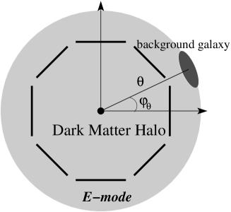
Figure 1: Illustration of the shear pattern around an axially-symmetric halo. A background galaxy image is tangentially deformed with respect to the halo center, corresponding to a pure $E$ mode in the shear field.

For an axially-symmetric mass distribution, the shear amplitude can be expressed in terms of the convergence field as a function of the radius from the halo center (e.g., Miralda-Escude 1991):

$$\gamma_{M}(\theta)=\bar{\kappa}_{M}(\theta)-\kappa_{M}(\theta),$$ (15)

where $\bar{\kappa}_{M}$ is the mean surface mass density inside a circle of radius $\theta$: $\bar{\kappa}_{M}=(1/\pi\theta^{2})\int^{\theta}_{0}~{}2\pi\theta^{\prime}d\theta^{\prime}~{}\kappa_{M}(\theta^{\prime})$. The equation above reflects the non-local nature of the shear field, since it is induced by non-local tidal forces. The shear field does not vanish outside the projected virial region because $\bar{\kappa}_{M}$ is non-zero, even if $\kappa_{M}(\theta)=0$. From equation (13), the shear profile for an NFW halo of mass $M$ can be analytically expressed as

$$\gamma_{M}(\theta)=4\pi Ga^{-1}\frac{d_{A}(\chi)d_{A}(\chi_{s}-\chi)}{d_{A}(\chi_{s})}\frac{Mfc^{2}}{2\pi r_{\rm vir}^{2}}G(c\theta/\theta_{\rm vir}),$$ (16)

with

$$G(x)=\left\{\begin{array}[]{ll}\displaystyle\frac{1}{x^{2}(1+c)}\left[\frac{(2-x^{2})\sqrt{c^{2}-x^{2}}}{1-x^{2}}-2c\right]+\frac{2}{x^{2}}\ln\frac{x(1+c)}{c+\sqrt{c^{2}-x^{2}}}+\frac{2-3x^{2}}{x^{2}(1-x^{2})^{3/2}}{\rm arccosh}\frac{x^{2}+c}{x(1+c)},&(x<1)\\ \displaystyle\frac{1}{3(1+c)}\left[\frac{(11c+10)\sqrt{c^{2}-1}}{1+c}-6c\right]+2\ln\frac{1+c}{c+\sqrt{c^{2}-1}},&(x=1)\\ \displaystyle\frac{1}{x^{2}(1+c)}\left[\frac{(2-x^{2})\sqrt{c^{2}-x^{2}}}{1-x^{2}}-2c\right]+\frac{2}{x^{2}}\ln\frac{x(1+c)}{c+\sqrt{c^{2}-x^{2}}}-\frac{2-3x^{2}}{x^{2}(x^{2}-1)^{3/2}}{\rm arccos}\frac{x^{2}+c}{x(1+c)},&(1<x\leq c)\\ \displaystyle\frac{2f^{-1}}{x^{2}},&(x>c).\end{array}\right.$$ (21)

where $f=1/[\ln(1+c)-c/(1+c)]$. Note the asymptotic behavior $G(x)\rightarrow 1/2$ for $x\rightarrow 0$, while the convergence $\kappa_{M}\rightarrow\infty$ in this limit (following from the NFW inner slope $\rho_{h}\propto r^{-1}$). This feature is in contrast to the case of a power law density profile $\rho_{h}\propto r^{-n}$ ($1<n\leq 3$), which leads to $\kappa_{M},\gamma_{M}\propto\theta^{1-n}$ and the asymptotic behavior $\kappa_{M},\gamma_{M}\rightarrow\infty$ for $\theta\rightarrow 0$. Outside the virial region the shear amplitude behaves like the field around a point mass, $\gamma_{M}\propto 1/\theta^{2}$, due to the sharp cutoff of the mass distribution. Taking $c\rightarrow\infty$ in the equation above leads to the expression for $\gamma_{M}$ in Bartelmann (1996; also see Wright & Brainerd 2000), which is derived from a line-of-sight projection of the NFW profile under the assumption that the profile is valid for an infinite range beyond the virial region. As shown in Figure 21, if one adopts the expression for $\gamma_{M}$ in Bartelmann (1996) the amplitude of shear correlations is significantly overestimated. Therefore, the halo profile boundary should be carefully considered to obtain accurate results as well as a consistent formulation.

The sketch in Figure 1 illustrates how a background galaxy image is tangentially deformed around a foreground lens with an axially-symmetric profile. In the weak lensing regime, the shear pattern is described by a pure $E$-mode. In Cartesian coordinates with the center taken as the halo center, the two shear components can be expressed as

$$\gamma_{M,1}(\mbox{{\it\boldmath$\theta$}})=-\gamma_{M}(\theta)\cos 2\varphi_{\mbox{{\it\boldmath$\theta$}}},\hskip 20.00003pt\gamma_{M,2}(\mbox{{\it\boldmath$\theta$}})=-\gamma_{M}(\theta)\sin 2\varphi_{\mbox{{\it\boldmath$\theta$}}},$$ (22)

where $\varphi_{\mbox{{\it\boldmath$\theta$}}}$ is the angle between the first x-axis and the line connecting the halo center and the source galaxy position (see Figure 1).

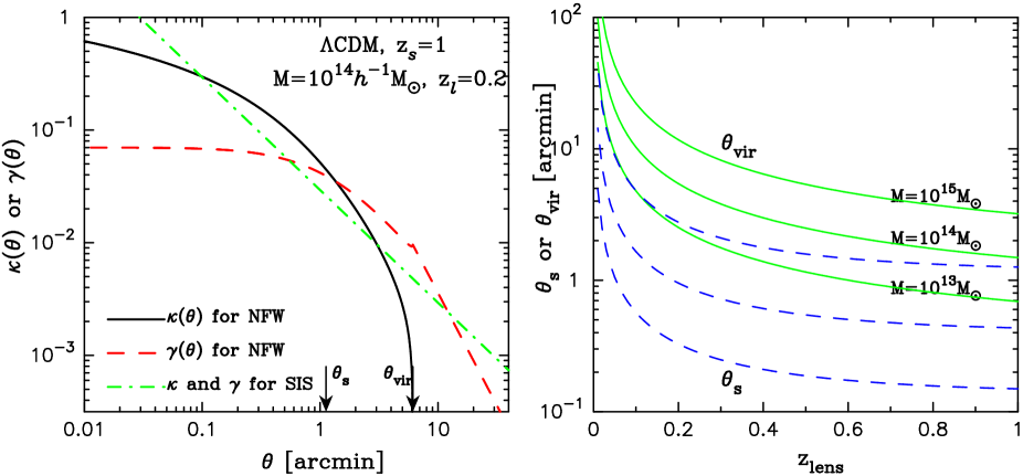
Figure 2: Left panel: Radial profiles of the convergence (solid curve) and shear (dashed curve) fields for an NFW halo. The halo mass is $M=10^{14}h^{-1}M_{\odot}$, lens redshift $z_{l}=0.2$ and source redshift $z_{s}=1$. For comparison, the dot-dashed curve shows a singular isothermal sphere $(\rho_{h}\propto r^{-2})$ with the same virial mass. The two arrows show the scale radius and the virial radius of the NFW profile. Right panel: The angular scales of the scale and virial radii for a lens halo are plotted against its redshift. The three curves show the results for halo masses $M/M_{\odot}=10^{13}$, $10^{14}$ and $10^{15}$, from bottom to top. Halos relevant for lensing statistics have $\theta_{\rm s}\lower 2.15277pt\hbox{$\;\buildrel<\over{\sim}\;$}2^{\prime}$ for their scale radii at redshift $z=0.4$. Thus the effect of the inner structures of the halo profile on lensing statistics should appear at scales $\lower 2.15277pt\hbox{$\;\buildrel<\over{\sim}\;$}2^{\prime}$.

The left plot in Figure 2 shows the radial profiles of the convergence (solid curve) and shear (dashed curve) for an NFW halo of mass $10^{14}h^{-1}M_{\odot}$, computed using equations (13) and (16). We use the $\Lambda$CDM model, lens redshift $z_{l}=0.2$ and source redshift $z_{s}=1$. The two arrows denote the angular scales $\theta_{s}$ and $\theta_{\rm vir}$ corresponding to the scale radius and the virial radius, respectively. In contrast to the convergence, the shear is almost constant in the inner region and does not vanish for $\theta\geq\theta_{\rm vir}$, rather it follows the point mass profile $\propto\theta^{-2}$. It should be noted that the shear profile appears to be not a smoothly varying function at $\theta=\theta_{\rm vir}$ because of the artificial sharp halo boundary. For comparison, the dot-dashed curve shows the shear amplitude for a singular isothermal sphere (SIS) with the profile $\rho_{h}\propto r^{-2}$ (for this case the convergence and shear fields coincide). The comparison manifests the characteristic feature for the NFW shear field. For example, the plateau profile, $\gamma_{M}\approx{\rm constant}$, at $\theta\lower 2.15277pt\hbox{$\;\buildrel<\over{\sim}\;$}\theta_{s}$ could be a direct test of the inner slope $\rho_{h}\propto r^{-1}$.

The right panel in Figure 2 explicitly shows the angular scales of the scale and virial radii for lens halos as a function of redshift. We consider the mass scales, $M/M_{\odot}=10^{13}$, $10^{14}$ and $10^{15}$. Halos with $M>10^{13}M_{\odot}$, which dominate the contribution to lensing statistics on small, non-linear scales, have $\theta_{\rm s}\lower 2.15277pt\hbox{$\;\buildrel<\over{\sim}\;$}2^{\prime}$ for their scale radii at redshift $z=0.4$. Thus, the figure implies that the the inner region likely affects the lensing statistics on angular scales $\lower 2.15277pt\hbox{$\;\buildrel<\over{\sim}\;$}2^{\prime}$, as we will show explicitly in Figure 13.

2.4 Real-space halo approach

In the halo model, the 2PCF of the convergence field, $\xi_{\kappa}(\theta)$, can be expressed as the sum of correlations within a single halo (1-halo term) and between two halos (2-halo term). In TJ03b, we obtained the real-space relation for the 1-halo term:

$$\xi^{1h}_{\kappa}(\theta)\equiv\langle{\kappa(\mbox{{\it\boldmath$\theta$}}_{1})\kappa(\mbox{{\it\boldmath$\theta$}}_{2})}\rangle^{1h}=\int^{\chi_{s}}_{0}\!\!d\chi~{}\frac{d^{2}V}{d\chi d\Omega}\int\!\!dM~{}n(M;\chi)\int_{0}^{\theta_{\rm vir}}\!\!ds\int^{2\pi}_{0}\!\!d\varphi~{}s~{}\kappa_{M}(s;\chi)\kappa_{M}(|\mbox{{\it\boldmath$s$}}+\mbox{{\it\boldmath$\theta$}}|;\chi),$$ (23)

where $d^{2}V/d\chi d\Omega=d_{A}^{2}(\chi)$ for a flat universe, and we have used polar coordinate $\mbox{{\it\boldmath$s$}}=s(\cos\varphi,\sin\varphi)$ to write $d^{2}\mbox{{\it\boldmath$s$}}=sdsd\varphi$. $\langle{\cdots}\rangle$ denotes the ensemble average. From statistical symmetry, we can set the separation vector $\theta$ to be along the first axis, so that $|\mbox{{\it\boldmath$s$}}+\mbox{{\it\boldmath$\theta$}}|=(s^{2}+\theta^{2}+2s\theta\cos\varphi)^{1/2}$. To obtain $\xi^{1h}_{\kappa}$ for a given cosmological model, we perform a 4-dimensional numerical integration. Equation (23) shows that $\xi_{\kappa}^{1h}$ is given by the sum of lensing contributions due to halos along the line of sight weighted with the halo number density on the light cone. Hence, this form correctly accounts for multiple lensing due to halos at different redshifts.

Figure 3 plots the angular number density of halos more massive than a given mass scale $M$ between the source redshift $z_{s}=1$ and the present: $N(>M)=\int^{z_{s}}_{0}\!\!dz~{}d^{2}V/(dzd\Omega)\int_{M}^{\infty}\!\!dM^{\prime}~{}n(M^{\prime};z)$. One can see $N(>M)\lower 2.15277pt\hbox{$\;\buildrel<\over{\sim}\;$}10^{-1}$ arcmin^-2 for halos with $M>10^{13}M_{\odot}$, which provide dominant contribution to the lensing statistics on small angular scales (see Figure 14). This clarifies that the 1-halo contribution is primarily due to a single lens halo, and that there is only a small probability for multiple lensing due to such massive halos at different redshifts. However, one should keep mind the importance of multiple lensing due to such cluster-scale halos and less massive halos, as shown by White, Van Waerbeke & Mackey (2002) and Padmanabhan, Seljak & Pen (2003).

Figure 3: Projected number density of halos more massive than a given mass scale $M$, $N(>M)$, between $z=0$ and $1$ for the $\Lambda$CDM model.

The form of equation (23) allows us to straightforwardly extend it to compute the 2PCF of shear fields by replacing the convergence profile, $\kappa_{M}$, with the shear profile, $\gamma_{M}$, for a given halo. The 1-halo term in Cartesian coordinates is

$$\langle{\gamma_{\mu}(\mbox{{\it\boldmath$\theta$}}_{1})\gamma_{\nu}(\mbox{{\it\boldmath$\theta$}}_{2})}\rangle^{1h}=\int^{\chi_{s}}_{0}\!\!d\chi~{}d_{A}^{2}(\chi)\int\!\!dM~{}n(M;\chi)\int_{0}^{\infty}\!\!ds\int^{2\pi}_{0}d\varphi~{}s~{}\gamma_{M}(s;\chi)\gamma_{M}(|\mbox{{\it\boldmath$s$}}+\mbox{{\it\boldmath$\theta$}}|;\chi)\epsilon_{\mu}(\mbox{{\it\boldmath$s$}})\epsilon_{\nu}(\mbox{{\it\boldmath$s$}}+\mbox{{\it\boldmath$\theta$}}),$$ (24)

where $\epsilon_{\mu}$ is the phase factor of the shear field as given by equation (5); $\epsilon_{\mu}(\mbox{{\it\boldmath$s$}})=-(\cos 2\varphi,\sin 2\varphi)$ and $\epsilon_{\mu}(\mbox{{\it\boldmath$s$}}+\mbox{{\it\boldmath$\theta$}})\equiv-(\cos 2\varphi_{\mbox{{\it\boldmath$s$}}+\mbox{{\it\boldmath$\theta$}}},\sin 2\varphi_{\mbox{{\it\boldmath$s$}}+\mbox{{\it\boldmath$\theta$}}})$ with $(\cos\varphi_{\mbox{{\it\boldmath$s$}}+\mbox{{\it\boldmath$\theta$}}},\sin\varphi_{\mbox{{\it\boldmath$s$}}+\mbox{{\it\boldmath$\theta$}}})=-|\mbox{{\it\boldmath$s$}}+\mbox{{\it\boldmath$\theta$}}|^{-1}(s\cos\varphi+\theta,s\sin\varphi)$. In contrast to equation (23), the equation above employs an infinite integration range for $d^{2}\mbox{{\it\boldmath$s$}}$ in order to account for the non-local property of the shear fields. In practice, setting the upper bound of $\int\!\!ds$ to be three times the projected virial radius gives the same result, to within a few percent. We investigate the accuracy of equation (24) as well as its self-consistency with other methods in §A.

Since the two shear components are not invariant under coordinate rotation, the shear 2PCFs generally depend on the relative orientation of the two points (e.g., Kaiser 1992). This issue has been well studied in the literature (Kamionkowski et al. 1998; Crittenden et al. 2002; Schneider et al. 2002a). One way to avoid the coordinate dependence is to use the $+/\times$ decompositions, where the $+$ component is defined as the shear field in parallel or perpendicular direction relative to the line connecting the two points taken, while the $\times$ component is the $45^{\circ}$ rotated shear field. We can thus define the rotationally invariant 2PCFs of the shear field:

$$\xi_{\gamma,+}(\theta) = \langle{\gamma_{+}(\mbox{{\it\boldmath$\theta$}}_{1})\gamma_{+}(\mbox{{\it\boldmath$\theta$}}_{2})}\rangle,$$

$$\xi_{\gamma,\times}(\theta) = \langle{\gamma_{\times}(\mbox{{\it\boldmath$\theta$}}_{1})\gamma_{\times}(\mbox{{\it\boldmath$\theta$}}_{2})}\rangle.$$ (25)

It should be noted that $\langle{\gamma_{+}(\mbox{{\it\boldmath$\theta$}}_{1})\gamma_{\times}(\mbox{{\it\boldmath$\theta$}}_{2})}\rangle$ and $\langle{\gamma_{\times}(\mbox{{\it\boldmath$\theta$}}_{1})\gamma_{+}(\mbox{{\it\boldmath$\theta$}}_{2})}\rangle$ vanish because of invariance under parity transformation. We will also consider the following 2PCF:

$$\xi_{\gamma}(\theta)=\langle{\mbox{{\it\boldmath$\gamma$}}(\mbox{{\it\boldmath$\theta$}}_{1})\cdot\mbox{{\it\boldmath$\gamma$}}^{\ast}(\mbox{{\it\boldmath$\theta$}}_{2})}\rangle.$$ (26)

Note that $\xi_{\kappa}(\theta)=\xi_{\gamma}(\theta)$. The 1-halo term contributions to these shear 2PCFs can be calculated by replacing the phase factors $\epsilon_{\mu}\epsilon_{\nu}$ in equation (24) with

$$\epsilon_{\mu}(\mbox{{\it\boldmath$s$}})\epsilon_{\nu}(\mbox{{\it\boldmath$s$}}+\mbox{{\it\boldmath$\theta$}})\rightarrow\left\{\begin{array}[]{ll}\cos 2\varphi\cos 2\varphi_{\mbox{{\it\boldmath$s$}}+\mbox{{\it\boldmath$\theta$}}}+\sin 2\varphi\sin 2\varphi_{\mbox{{\it\boldmath$s$}}+\mbox{{\it\boldmath$\theta$}}},&\mbox{for }~{}\xi_{\gamma},\\ \cos 2\varphi\cos 2\varphi_{\mbox{{\it\boldmath$s$}}+\mbox{{\it\boldmath$\theta$}}},&\mbox{for }~{}\xi_{\gamma,+},\\ \sin 2\varphi\sin 2\varphi_{\mbox{{\it\boldmath$s$}}+\mbox{{\it\boldmath$\theta$}}},&\mbox{for }~{}\xi_{\gamma,\times},\end{array}\right.$$ (30)

An alternative approach to the lensing 2PCF, which is conventionally used in the literature, is based on a model of the non-linear 3D power spectrum of the mass, $P(k)$. Combining $P(k)$ with Limber’s approximation (Limber 1954; Kaiser 1992) allows us to compute the shear 2PCFs:

$$\langle{\gamma_{\mu}\gamma_{\nu}}\rangle(\theta)=\int^{\chi_{s}}_{0}\!\!d\chi~{}W^{2}(\chi,\chi_{s})d_{A}^{-2}(\chi)\int\!\!\frac{ldl}{2\pi}~{}P\!\left(k=\frac{l}{d_{A}(\chi)}\right)F(l\theta).$$ (31)

Setting the window function to $F(x)=J_{0}(x)$, $[J_{0}(x)+J_{4}(x)]/2$ and $[J_{0}(x)-J_{4}(x)]/2$ yields $\xi_{\gamma}$, $\xi_{\gamma,+}$ and $\xi_{\gamma,\times}$, respectively. So far, there are two well studied models for the nonlinear $P(k)$. One is the fitting formula calibrated from $N$-body simulations (e.g., Jain, Mo & White 1995, Peacock & Dodds 1996, and Smith et al. 2002). This method has been extensively used for the interpretation of cosmic shear measurements in terms of cosmological parameters (e.g., Van Waerbeke 2001b). The other is the recently developed Fourier-space halo approach (Seljak 2000; Ma & Fry 2000b,c; Scoccimarro et al. 2001). In the halo model, $P(k)$ is similarly expressed as sum of the 1- and 2-halo terms; $P(k)=P_{1h}(k)+P_{2h}(k)$ (see §2.2 in TJ0b for details). Inserting $P_{1h}(k)$ into equation (31) leads to the 1-halo term of the shear 2PCFs in the Fourier-space halo model. Note that the condition $\xi_{\kappa}=\xi_{\gamma}$ holds, since they both have the same window function $J_{0}$ in equation (31).

Figure 4: Upper: A sketch of the triangle configuration, parameterized by $r$, $q$ and $\psi$, used to describe the 3PCF. The solid and dashed lines at each vertex show the positive directions of the $+$ and $\times$ components of the shear field, defined with respect to the triangle center denoted by $o$. Lower: The mirror transformation of the triangle with respect to the side vector $r$ for $\xi_{\times++}$ is shown as one example. The $\gamma_{\times}$ component at each vertex changes sign under the mirror transformation (at vertices $1$ and $1^{\prime}$ in this case).

We turn to the 3PCF of lensing fields, which is main focus of this paper. The 1-halo term of the 3PCF of the convergence field is given by equation (52) in TJ03b:

$$\zeta^{1h}_{\kappa}(r,q,\psi)\equiv\langle{\kappa(\mbox{{\it\boldmath$\theta$}}_{1})\kappa(\mbox{{\it\boldmath$\theta$}}_{2})\kappa(\mbox{{\it\boldmath$\theta$}}_{3})}\rangle^{1h}=\int^{\chi_{s}}_{0}\!\!d\chi~{}d_{A}^{2}(\chi)\int\!\!dM~{}n(M;\chi)\int^{\theta_{\rm vir}}_{0}\!\!ds\int_{0}^{2\pi}\!\!d\varphi~{}s~{}\kappa_{M}(s)\kappa_{M}(|\mbox{{\it\boldmath$s$}}+\mbox{{\it\boldmath$r$}}|)\kappa_{M}(|\mbox{{\it\boldmath$s$}}+\mbox{{\it\boldmath$q$}}|),$$ (32)

where we have set $|\mbox{{\it\boldmath$s$}}+\mbox{{\it\boldmath$r$}}|=(s^{2}+r^{2}+2rs\cos\varphi)^{1/2}$ and $|\mbox{{\it\boldmath$s$}}+\mbox{{\it\boldmath$q$}}|=[s^{2}+q^{2}+2sq\cos(\varphi-\psi)]^{1/2}$. From statistical symmetry, the convergence 3PCF can be expressed as a function of three parameters $r$, $q$ and $\psi$ characterizing the triangle configuration, as shown in Figure 4. Note that we often omit $\chi$ in the argument of $\kappa_{M}$ or $\gamma_{M}$ for simplicity. This equation means that we can compute $\zeta^{1h}_{\kappa}$ by a 4-dimensional integration for any triangle configuration, which is the same level of computation as the 2PCF. This holds for higher-order moments as well (TJ03b), which is a great advantage of the real-space halo model. For comparison, the Fourier-space halo model requires a 6-dimensional integration to get $\zeta^{1h}_{\kappa}$. In TJ03b, we have also developed approximations for computing the 2- and 3-halo terms of $\zeta_{\kappa}$. The 2-halo term is relevant for a range of transition scales between the non-linear and quasi-nonlinear regimes, while the 3-halo term dominates in the large scale, quasi-linear regime where perturbation theory (PT) is valid.

We can extend equation (32) to the shear 3PCFs. Since the shear field has two components at each vertex of a given triangle configuration, we can formally construct eight ($2^{3}=8$) components of the shear 3PCFs. In Cartesian coordinates the functions are

$$\zeta_{\gamma,abc}(\mbox{{\it\boldmath$\theta$}}_{1},\mbox{{\it\boldmath$\theta$}}_{2},\mbox{{\it\boldmath$\theta$}}_{3})\equiv\langle{\gamma_{a}(\mbox{{\it\boldmath$\theta$}}_{1})\gamma_{b}(\mbox{{\it\boldmath$\theta$}}_{2})\gamma_{c}(\mbox{{\it\boldmath$\theta$}}_{3})}\rangle,$$ (33)

where $a,b,c=1,2$. Note that the subscripts $a,b,c$ correspond to the shear components at vertices $\mbox{{\it\boldmath$\theta$}}_{1}$, $\mbox{{\it\boldmath$\theta$}}_{2}$ and $\mbox{{\it\boldmath$\theta$}}_{3}$, respectively, in our convention (see Figure 4). As for the shear 2PCFs, the 3PCFs defined above are not invariant under coordinate rotation. Therefore, in contrast to the 3PCF of the convergence or any scalar quantity, they are not specified by three parameters. Instead four parameters are needed, e.g., $r$, $q$, $\psi$ and the orientation angle of the side vector $r$ relative to the first coordinate axis. The real-space halo model yields the following expressions for the 1-halo terms of the shear 3PCFs:

$$\zeta^{1h}_{\gamma,abc}(\mbox{{\it\boldmath$r$}},\mbox{{\it\boldmath$q$}}) = \int^{\chi_{s}}_{0}\!\!d\chi~{}d_{A}^{2}(\chi)\int\!\!dM~{}n(M;\chi)\int^{\infty}_{0}\!\!ds\int_{0}^{2\pi}\!\!d\varphi~{}s~{}\gamma_{M}(s)\gamma_{M}(|\mbox{{\it\boldmath$s$}}+\mbox{{\it\boldmath$r$}}|)\gamma_{M}(|\mbox{{\it\boldmath$s$}}+\mbox{{\it\boldmath$q$}}|)\epsilon_{a}(\mbox{{\it\boldmath$s$}})\epsilon_{b}(\mbox{{\it\boldmath$s$}}+\mbox{{\it\boldmath$r$}})\epsilon_{c}(\mbox{{\it\boldmath$s$}}+\mbox{{\it\boldmath$q$}}),$$ (34)

with

$$\epsilon_{a}({\mbox{{\it\boldmath$s$}}}) = -(\cos 2\varphi,\sin 2\varphi),$$

$$\epsilon_{b}(\mbox{{\it\boldmath$s$}}+\mbox{{\it\boldmath$r$}}) = -(\cos 2\varphi_{\mbox{{\it\boldmath$s$}}+\mbox{{\it\boldmath$r$}}},\sin 2\varphi_{\mbox{{\it\boldmath$s$}}+\mbox{{\it\boldmath$r$}}}),$$

$$\epsilon_{c}(\mbox{{\it\boldmath$s$}}+\mbox{{\it\boldmath$q$}}) = -(\cos 2\varphi_{\mbox{{\it\boldmath$s$}}+\mbox{{\it\boldmath$q$}}},\sin 2\varphi_{\mbox{{\it\boldmath$s$}}+\mbox{{\it\boldmath$q$}}})$$ (35)

where $(\cos\varphi_{\mbox{{\it\boldmath$s$}}+\mbox{{\it\boldmath$r$}}},\sin\varphi_{\mbox{{\it\boldmath$s$}}+\mbox{{\it\boldmath$r$}}})=(r+s\cos\varphi,s\sin\varphi)/|\mbox{{\it\boldmath$s$}}+\mbox{{\it\boldmath$r$}}|$, $(\cos\varphi_{\mbox{{\it\boldmath$s$}}+\mbox{{\it\boldmath$q$}}},\sin\varphi_{\mbox{{\it\boldmath$s$}}+\mbox{{\it\boldmath$q$}}})=(q\cos\psi+s\cos\varphi,q\sin\psi+s\sin\varphi)/|\mbox{{\it\boldmath$s$}}+\mbox{{\it\boldmath$q$}}|$, $|\mbox{{\it\boldmath$s$}}+\mbox{{\it\boldmath$r$}}|$ and $|\mbox{{\it\boldmath$s$}}+\mbox{{\it\boldmath$q$}}|$ are given below equation (32), and we again take the halo center as the coordinate center, using statistical symmetry.

To avoid the coordinate dependence for the shear 3PCFs, we again use the $+/\times$ decomposition of the shear fields, as stressed in SL03. For the three-point case, however, there is no unique choice of the reference direction to define the $+/\times$ components. Following ZS03 and TJ03a, we take the ‘center of mass’, $o$, of the triangle, defined by

$$\mbox{{\it\boldmath$o$}}=\frac{1}{3}\sum_{i=1}^{3}\mbox{{\it\boldmath$\theta$}}_{i}=\mbox{{\it\boldmath$s$}}+\frac{1}{3}(r+q\cos\psi,q\sin\psi).$$ (36)

The projection operators, which transform $\gamma_{1}$ and $\gamma_{2}$ at each vertex into the $+/\times$ components, with respect to $o$, are

$$\mbox{{\it\boldmath$P$}}_{+}(\mbox{{\it\boldmath$\theta$}}_{i})=-(\tilde{\theta}_{i1}^{2}-\tilde{\theta}_{i2}^{2},2\tilde{\theta}_{i1}\tilde{\theta}_{i2})/\tilde{\theta}_{i}^{2},\hskip 20.00003pt\mbox{{\it\boldmath$P$}}_{\times}(\mbox{{\it\boldmath$\theta$}}_{i})=-(-2\tilde{\theta}_{i1}\tilde{\theta}_{i2},\tilde{\theta}_{i1}^{2}-\tilde{\theta}_{i2}^{2})/\tilde{\theta}_{i}^{2},$$ (37)

where $\tilde{\mbox{{\it\boldmath$\theta$}}}_{i}=\mbox{{\it\boldmath$\theta$}}_{i}-\mbox{{\it\boldmath$o$}}$ ($i=1,2,3$). The geometry of the triangle we consider is illustrated in Figure 4, where the solid and dashed lines at each vertex denote positive directions of the $+$ and $\times$ components. Using these projections, we can thus define the shear 3PCFs from combinations of the $+/\times$ components so that the resulting 3PCFs are invariant under rotations of the triangle with respect to $o$:

$$\zeta_{\gamma,\nu\mu\tau}(r,q,\psi)=P_{\mu}^{a}(\mbox{{\it\boldmath$\theta$}}_{1})P_{\nu}^{b}(\mbox{{\it\boldmath$\theta$}}_{2})P_{\tau}^{c}(\mbox{{\it\boldmath$\theta$}}_{3})\langle{\gamma_{a}(\mbox{{\it\boldmath$\theta$}}_{1})\gamma_{b}(\mbox{{\it\boldmath$\theta$}}_{2})\gamma_{c}(\mbox{{\it\boldmath$\theta$}}_{3})}\rangle,$$ (38)

where $\mu,\nu,\tau=+$ or $\times$. Inserting equation (34) into the r.h.s above yields the 1-halo term for $\zeta_{\gamma,\nu\mu\tau}$. The projection operators and $\langle{\cdots}\rangle$ commute, since the projection operators do not depend on the integration variable $s$, as seen from equation (37). The shear 3PCFs defined in this way are functions of the three parameters $r$, $q$ and $\psi$. Although we adopt the center of mass throughout this paper, SL03 proved that the eight shear 3PCFs with respect to any center can be expressed as linear combinations of the eight 3PCFs above. To complete the halo model predictions, it is necessary to develop the perturbation theory predictions for the shear 3PCFs, which are relevant on large scales. For the convergence we have obtained these, but the complex spin-2 properties of the shear fields make it non-trivial to obtain the PT prediction. We will consider only the 1-halo term for predictions of the shear 3PCFs. Nevertheless, the 1-halo term agrees with the simulation results on scales of interest, as shown below.

3 Triangle configuration dependences of the shear 3PCF

From the observation that there are eight shear 3PCFs, SL03 and ZS03 addressed the questions: how many functions are non-zero? How does each function carry information about the $E/B$-modes? In TJ03a, using ray-tracing simulations, we qualitatively verified the conclusions of SL03 and ZS03, which were based on analytical studies. We found that: (1) The eight 3PCFs are generally non-zero. (2) For a pure $E$-mode, two or four components vanish for isosceles or equilateral triangles, respectively. (3) We also studied the triangle configuration dependence of the shear 3PCF given by equation (43), and pointed out that they offer a promising way to disentangle the $E/B$-modes for measured shear 3PCFs. Here we summarize these characteristics of the shear 3PCFs.

We restrict ourselves to a pure $E$ field, expected in the weak lensing regime. We consider a mirror transformation as shown in Figure 4, which illustrates the transformation with respect to the side vector $r$ for $\zeta_{\times++}$. It corresponds to $\psi\rightarrow 2\pi-\psi$ in our parameterization. From statistical homogeneity and symmetry, the amplitude of the shear 3PCF depends only on the distances between the center and each vertex. Hence, the absolute amplitudes of $\zeta_{\times++}$ for the two triangles shown should be same. But the sign of $\gamma_{\times}$ at the vertex $1^{\prime}$ changes under this mirror transformation. According to this property, we can divide the eight 3PCFs into two groups:

Parity-even functions: $$\zeta_{\mu\nu\tau}(r,q,\psi)=\zeta_{\mu\nu\tau}(r,q,2\pi-\psi),\mbox{ for }\ \ (\mu,\nu,\tau)=(+,+,+),(+,\times,\times),(\times,+,\times),(\times,\times,+),$$

Parity-odd functions: $$\zeta_{\mu\nu\tau}(r,q,\psi)=-\zeta_{\mu\nu\tau}(r,q,2\pi-\psi),\mbox{ for }\ \ (\mu,\nu,\tau)=(\times,\times,\times),(\times,+,+),(+,\times,+),(+,+,\times).$$ (39)

Note that the 3PCF of a scalar quantity transforms as $\zeta(r,q,\psi)=\zeta(r,q,2\pi-\psi)$.

Next we consider special triangle configurations: the first is an isosceles triangle with $r=q$. In this case, the $\gamma_{\times}$ components at vertices $1$ and $1^{\prime}$ in Figure 4 are statistically identical (viewed from the center of the triangle, they should have equal contributions when averaged over the matter distribution). We thus have additional symmetries for the two 3PCFs: $\zeta_{\times++}(r,q,\psi)=\zeta_{\times++}(r,q,2\pi-\psi)$ and $\zeta_{\times\times\times}(x_{1},x_{1},\psi)=\zeta_{\times\times\times}(x_{1},x_{1},2\pi-\psi)$. These relations and equation (39) yield

$$\mbox{Isosceles Triangles: }\ \ \zeta_{\times++}=\zeta_{\times\times\times}=0.$$ (40)

Note that the other two parity-odd functions, $\zeta_{+\times+}$ and $\zeta_{++\times}$, do not vanish in general, since the component $\gamma_{\times}$ is at a vertex bounded by unequal sides. For equilateral triangles, however, all four parity-odd functions vanish:

$${\rm Equilateral\ Triangles:}\ \ \zeta_{\times\times\times}=\zeta_{\times++}=\zeta_{+\times+}=\zeta_{++\times}=0.$$ (41)

The 3PCFs discussed above do not vanishing for a $B$-mode shear field, as explained below. Hence these 3PCFs provide a direct, simple test of the $B$-mode contribution to the measured signal.

Let us consider again generic triangle configurations, but now for a pure $B$ field. As discussed by TJ03a, the analog of equation (39) for a B-mode spin-2 field is:

$$\zeta_{\mu\nu\tau}(r,q,\psi)=-\zeta_{\mu\nu\tau}(r,q,2\pi-\psi),\mbox{ for }\ \ (\mu,\nu,\tau)=(+,+,+),(+,\times,\times),(\times,+,\times),(\times,\times,+),$$

$$\zeta_{\mu\nu\tau}(r,q,\psi)=\zeta_{\mu\nu\tau}(r,q,2\pi-\psi),\mbox{ for }\ \ (\mu,\nu,\tau)=(\times,\times,\times),(\times,+,+),(+,\times,+),(+,+,\times).$$ (42)

Thus the symmetric and anti-symmetric functions are reversed compared to the $E$-mode. This follows from the fact that given a pure $E$ field, we can generate a pure $B$ field by rotating the $E$ field at each point by $45$ degrees (Kaiser 1992). We can then consider the eight 3PCFs of a pure $B$ mode similarly as done for the shear 3PCFs. Since this procedure transforms the original $E$-mode components $\gamma^{E}_{+}$ and $\gamma^{E}_{\times}$ at each point into $\gamma^{B}_{\times}$ and $\gamma^{B}_{+}$ in the transformed $B$ field, respectively, we get $\zeta^{E}_{+++}\rightarrow\zeta^{B}_{\times\times\times}$ and so on. For a general spin-2 field that contains both $E/B$ modes, the configuration dependences of equations (39) and (42) do not hold. The eight 3PCFs therefore have to be measured over the full range $\psi=[0,2\pi]$, unlike the 3PCF of a scalar quantity.

From the symmetry properties discussed above, we propose simple estimators for the $E/B$-mode contributions to measured shear 3PCFs:

$$\mbox{Estimator of $E$-mode}: {\displaystyle\zeta^{E}_{\mu\nu\tau}(r,q,\psi)=\frac{1}{2}\left[\zeta_{\gamma,\mu\nu\tau}(r,q,\psi)\pm\zeta_{\gamma,\mu\nu\tau}(r,q,2\pi-\psi)\right]},$$

$$\mbox{Estimator of $B$-mode}: {\displaystyle\zeta^{B}_{\mu\nu\tau}(r,q,\psi)=\frac{1}{2}\left[\zeta_{\gamma,\mu\nu\tau}(r,q,\psi)\mp\zeta_{\gamma,\mu\nu\tau}(r,q,2\pi-\psi)\right]},$$ (43)

where the upper and lower signs in $\pm$ or $\mp$ are meant for $(\mu,\nu,\tau)=(+,+,+),(+,\times,\times),(\times,+,\times),(\times,\times,+)$ and $(\times,\times,\times),(\times,+,+),(+,\times,+),(+,+,\times)$, respectively. Note that this argument holds if the $E$ and $B$ modes are statistically uncorrelated. These estimators allow one to separate the lensing $E$-mode contribution from the measured 3PCFs that are in general contaminated by the $B$-modes contribution of intrinsic alignments, source galaxy clustering and observational systematics. In comparison, for the case of the shear 2PCFs, a non-local integration is required to discriminate the lensing $E$-mode (Schneider et al. 1998; Crittenden et al. 2002; Schneider et al. 2002a).

After the submission of this paper, Schneider (2003) pointed out that if a $B$ field is parity invariant in a statistical sense, any correlation function that contains an odd number of $B$-mode shear components vanishes. This is likely to be true for a cosmological $B$ field such as intrinsic alignments if we have a sufficient survey area. Therefore, the argument we have made above is valid only for a parity non-invariant $B$ field. This can be seen in that the 45 degree rotation procedure described above to generate a $B$ field from simulations would produce shear fields around clusters with a clockwise curl direction, which violates statistical parity invariance. Nevertheless, we believe our discussion is useful, because generic observational systematics are likely lead to the violation of parity invariance. Hence, these arguments strength practical usefulness of the shear 3-point functions to disentangle $E/B$ modes from the measurement.

4 Comparison with ray-tracing simulations

In this section, we address the accuracy of the halo model for predicting lensing statistics, in particular the 3PCFs, by comparing model predictions with ray-tracing simulation results. The validity of the real-space halo model for shear correlations, developed in §2, is carefully investigated in §A.

4.1 Cosmological models

In this paper, we mainly consider two CDM models whose cosmological parameters are chosen to facilitate comparison with the ray-tracing simulations used below (Jain et al. 2000; Ménard et al. 2003; Hamana et al. 2003). One is the SCDM model ($\Omega_{m0}=1$, $h=0.5$ and $\sigma_{8}=0.6$), and the other is the $\Lambda$CDM model ($\Omega_{m0}=0.3$, $\Omega_{\lambda 0}=0.7$, $\Omega_{b0}=0.04$, $h=0.7$ and $\sigma_{8}=0.9$). For the $\Lambda$CDM model, we need to care about the baryon contribution to the input primordial power spectrum. Although we assume a scale-invariant power spectrum for the primordial fluctuations, we employ different CDM transfer functions for the SCDM and $\Lambda$CDM models. For the SCDM model, we use the transfer function in Bond & Efstathiou (1984) with the shape parameter $\Gamma=\Omega_{\rm m0}h=0.5$. On the other hand, for the $\Lambda$CDM model we employ the BBKS transfer function (Bardeen et al. 1986) with the shape parameter in Sugiyama (1995), since the shape parameter approximately describes the baryon contribution.

4.2 Ray-tracing simulations

We use ray-tracing simulations of the lensing convergence and shear fields. We will mainly consider two cosmological model simulations, the $\Lambda$CDM model (kindly made available to us by T. Hamana; see Ménard et al. 2003; Hamana et al. 2003 for details) and the SCDM model (Jain et al. 2000), as described in §4.1. The $N$-body simulations on which these are based were carried out by the Virgo Consortium (also see Yoshida, Sheth & Diaferio 2001), and were run using the particle-particle/particle-mesh (P³M) code with a force softening length of $l_{\rm soft}\sim 30h^{-1}$kpc. The linear power spectra of the initial conditions of the simulations were set up using the transfer function from CMBFast (Seljak & Zaldarriaga 1996) for the $\Lambda$CDM model and the fitting function in Bond & Efstathiou (1984) for the SCDM model, respectively. For the halo model predictions for $\Lambda$CDM , we employ the BBKS plus Sugiyama transfer function as described above. We verify in Figure 20 that the transfer function is sufficiently accurate (see also Eisenstein & Hu 1999).

The $\Lambda$CDM simulation employs $512^{3}$ CDM particles in a cubic box $479h^{-1}$Mpc on a side, while the SCDM simulation uses $256^{3}$ particles in a $84.5h^{-1}$Mpc side-length box. The particle mass is $m_{\rm part}=6.8\times 10^{10}h^{-1}M_{\odot}$ and $1.0\times 10^{10}h^{-1}M_{\odot}$, respectively. The resolution scale, which is not affected by the discreteness of the $N$-body simulations, is estimated roughly as being ten times the grid size, leading to $\lambda\lower 2.15277pt\hbox{$\;\buildrel>\over{\sim}\;$}94h^{-1}$kpc and $33h^{-1}$kpc for the $\Lambda$CDM and SCDM models, respectively. Therefore, the SCDM model simulation has better spatial resolution than the $\Lambda$CDM model.

The multiple-lens plane algorithm to simulate the lensing maps from the $N$-body simulations is detailed in Jain et al. (2000) and Hamana & Mellier (2001). Throughout this paper, we use a single source redshift of $z_{s}=1$. The simulated areas of the lensing maps are $\Omega_{s}=11.7$ and $7.69$ degree² for the $\Lambda$CDM and SCDM models, respectively. The map is given on $1024^{2}$ grids with grid spacing $\theta_{\rm grid}=0.\!\!^{\prime}2$ and $0.\!\!^{\prime}16$ for the two models. To analyze the correlation functions we should be careful about the possibility that the finite angular resolution could affect computations of the $n$-point correlation functions from the simulated maps on small scales. It is not easy to infer the effective angular resolution from the spatial resolution of the $N$-body simulations due to the broad lensing projection kernel. Further, the projected density field was smoothed to suppress the discreteness effect of the $N$-body simulations. The smoothing scale is likely to determine the angular resolution rather than the spatial resolution of the $N$-body simulation. Note that the $\Lambda$CDM simulation we employ below is the one labelled with small-scale smoothing in Ménard et al. (2003). These resolution issues were carefully discussed in Ménard et al. (2003) and Jain et al. (2000), as can be seen from Figure 3 in Ménard et al (2003) and Figure 2 in Jain et al. (2000). The former shows the projected angular scale of the smoothing as a function of redshift, while the latter shows the angular scale of the force-softening length of the $N$-body simulation. These scales are $\theta_{\rm res}\sim 0.\!\!^{\prime}3$ and $0.\!\!^{\prime}2$ at $z=0.4$ for the $\Lambda$CDM and SCDM models, respectively, where $z=0.4$ is approximately the peak redshift of the lensing efficiency for source redshift $z_{s}=1$. Therefore, angular scales that are not affected by finite resolution are likely to be $\lower 2.15277pt\hbox{$\;\buildrel>\over{\sim}\;$}1^{\prime}$, although the resolution of the $\Lambda$CDM model simulation might be slightly worse than that of the SCDM model, as stated above. We will keep in mind these resolution issues in the following analysis.

To compute the sample variance of the lensing statistics from the simulations, we use 36 and 9 realizations of the simulated lensing maps for the $\Lambda$CDM and SCDM models, respectively. The realizations are generated by randomly rotating and translating the N-body simulation boxes (using the periodic boundary conditions of the $N$-body boxes) when the ray-tracing simulations are performed. However, they were built from one realization of the $N$-body simulation, which is a sequence of the redshift-space evolution of large-scale structure. Therefore the different realizations of the simulated lensing maps are not fully independent of each other. In particular, this could matter when we compute the covariance for the $n$-point correlations in the different bins from the simulations. This issue is still an open question, to be addressed in the future using a sufficient number of truly independent ray-tracing simulations.

4.3 Algorithm for computing the 3PCF from simulated maps

To compute the 3PCFs of the lensing fields from the ray-tracing simulations, we implement the method described in §3.2.2 in Barriga & Gaztañaga (2002). The 3PCF is given as a function of three parameters ($r$, $q$ and $\psi$) specifying the triangle configuration (see Figure 4). The question is how we can efficiently find triplets from the simulated lensing map with $N_{\rm grid}$ grid points, subject to the constraint that the triplet forms a given triangle configuration within the bin widths. We first select vertex 1 on the grid, and then search vertex 2 in the upper half plane in an annulus of radius $r$ with given bin width, centered on vertex 1. For given pair 1-2, we look for vertex 3 in a semi-annulus of radius $q$ in the upper plane above the line connecting vertices $1$ and 2 (in the anticlockwise direction from vertex 1 as our convention), imposing the condition that the three vertices form the required triangle configuration within the bin widths. This results in all triangles being counted once, if we impose the conditions $\theta_{12}\leq\theta_{23}\leq\theta_{31}$. We can use the same list of neighbors to find vertices 2 and 3 for each vertex 1. This process is illustrated in Figure 3 in Barriga & Gaztañaga (2002). Further, to compute the 3PCFs of the shear fields, we need to compute the $+/\times$ components of the shear fields at each vertex of the triangle. The projection operators to compute these components are given as a function of the list of neighbors of vertices 2 and 3, independent of the position of vertex 1, as can be seen from the definition of equation (37). In summary, the 3PCF computation from the simulation map requires roughly $O(N_{\rm grid})$ operations on sufficiently small scales. This is significantly faster than a naive, direct implementation which requires $O(N_{\rm grid}^{3})$ operations.

4.4 The two-point correlation function of the shear fields

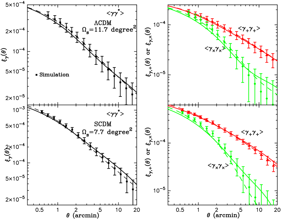
Figure 5: Comparison of model predictions for the shear 2PCFs with measurements from the ray-tracing simulations. The left panel shows the shear 2PCF, $\xi_{\gamma}=\langle{\mbox{{\it\boldmath$\gamma$}}\cdot\mbox{{\it\boldmath$\gamma$}}^{\ast}}\rangle$, for the $\Lambda$CDM (upper panel) and SCDM (lower panel) models. The solid and dashed curves are the predictions from the halo model and the Smith02 formula, respectively, while the square symbols with error bars denote the simulation result. Note that errors in different bins are highly correlated with each other. Similarly, the right panel shows the comparison for $\xi_{\gamma,+}$ and $\xi_{\gamma,\times}$.

In Figure 5 we present a comparison of the halo model predictions for the shear 2PCFs with those measured from the ray-tracing simulations for the $\Lambda$CDM (upper panel) and SCDM (lower panel) models. The left panel is the comparison for $\xi_{\gamma}$. The solid curve is the halo model prediction, while the square symbol denotes the simulation result. The dashed curve denotes the result computed from the Smith02 formula. The theoretical predictions agree very well with the simulation results for the two CDM models. The smallest scale data from the simulations corresponds to three times the grid size, and the error bar in each bin is the sample variance for area $\Omega=11.7$ and $7.7$ degree² for the $\Lambda$CDM and SCDM model simulations, respectively, as estimated from the scatter among their 36 and 9 realizations (see §4.2). We note that the errors in different bins are highly correlated with each other. Even if one combines two neighboring bins, the error amplitude remains almost unchanged. We have confirmed that this is true for all the statistical quantities we consider below, over angular scales of interest.

Similarly, the right panel in Figure 5 shows the comparison for $\xi_{+}$ and $\xi_{\times}$. The theoretical predictions for $\xi_{\gamma,+}$ are again in agreement with the simulation results. On the other hand, for $\xi_{\gamma,\times}$, the halo model prediction lies slightly below the simulation results at $\theta\lower 2.15277pt\hbox{$\;\buildrel<\over{\sim}\;$}5^{\prime}$, while the Smith02 prediction agrees better. If we employ the halo boundary of $r_{180}$ as discussed in Figure 21, the model predictions agree better with the simulations. The relation between the amplitudes of $\xi_{\gamma,+}$ and $\xi_{\gamma,\times}$ is physically determined by the $k$-slope of the underlying mass power spectrum, as can be seen from equation (31). Within the framework of the halo model, the slope is determined by the combined effects of the halo profile, the mass function and the slope of the primordial power spectrum (Seljak 2000; Ma & Fry 2000a,b,c; Scoccimarro et al. 2001; TJ02; TJ03b). Thus, separate measurements of $\xi_{+}$ and $\xi_{\times}$ could constrain these physical ingredients.

4.5 The three-point correlation function of the convergence field

In the following, we address the accuracy of halo model predictions for the 3PCFs of lensing fields by comparison with ray-tracing simulations. Until our recent work (TJ03a,b), there had been no analytical model for the lensing 3PCFs on small angular scales, except for investigations of the skewness and bispectrum of the convergence field based on extended perturbation theory (Scoccimarro & Frieman 1999; Hui 1999; Van Waerbeke et al. 2001a) or the Fourier-space halo model (Cooray & Hu 2001a; TJ02). Hence we present a detailed analysis of the accuracy of halo model predictions for the lensing 3PCFs.

First, we consider the 3PCF of the convergence field. As in the literature, we define the reduced 3PCF as

$$Q_{\kappa}(r,q,\psi)=\frac{\zeta_{\kappa}(r,q,\psi)}{\xi_{\kappa}(r)\xi_{\kappa}(q)+\xi_{\kappa}(r)\xi_{\kappa}(|\mbox{{\it\boldmath$r$}}-\mbox{{\it\boldmath$q$}}|)+\xi_{\kappa}(q)\xi_{\kappa}(|\mbox{{\it\boldmath$r$}}-\mbox{{\it\boldmath$q$}}|)},$$ (44)

where we have used the parameters $r$, $q$ and $\psi$ to describe the triangle configuration and $|\mbox{{\it\boldmath$r$}}-\mbox{{\it\boldmath$q$}}|=(r^{2}+q^{2}-2rq\cos\psi)^{1/2}$ (see Figure 4). The reduced 3PCF is sensitive to $\Omega_{\rm m0}$, but insensitive to the power spectrum normalization $\sigma_{8}$, scaling roughly as $Q_{\kappa}\propto\Omega_{\rm m0}^{-1}$ (Bernardeau et al. 1997; Jain & Seljak 1997; TJ02). Therefore, measuring the 3PCF is expected to break degeneracies in the determination of $\sigma_{8}$ and $\Omega_{\rm m0}$ from measurements of the shear 2PCFs.

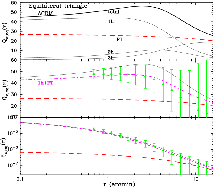
Figure 6: The 3PCF of the convergence field for equilateral triangles against side length $r$ in arcminutes. Top panel: The thick solid curve shows the halo model prediction for the reduced 3PCF, $Q_{\kappa}$, defined by equation (44). The thin solid curves denote the 1-, 2- and 3-halo term contributions separately. The dashed curve is the perturbation theory (PT) prediction. Middle panel: The comparison with simulations for $Q_{\kappa}$, as in Figure 5. The simulation result does not display the bump in $Q_{\kappa}$ seen in the halo model prediction. This is likely to be due to halo boundary effects in the standard implementation of the halo model (see text for details). The dot-dashed curve denotes the result if we replace the 2- and 3-halo terms with the PT prediction. This modified halo model agrees well with the simulation result. Bottom panel: The comparison for the 3PCF itself, as in the middle panel.

Figure 6 shows the convergence 3PCF for equilateral triangles against side length for the $\Lambda$CDM model. The thick solid curve in the top panel shows the halo model prediction for $Q_{\kappa}$. A bump feature is evident over the range $1\lower 2.15277pt\hbox{$\;\buildrel<\over{\sim}\;$}r\lower 2.15277pt\hbox{$\;\buildrel<\over{\sim}\;$}5^{\prime}$. As discussed below, this feature is unlikely to be real. The three thin curves show the 1-, 2- and 3-halo terms separately. These contributions to the convergence 3PCF are present in the numerator of $Q_{\kappa}$, but the 2PCF in the denominator includes the full contribution (1- plus 2-halo terms). The 1-halo term provides the dominant contribution to $Q_{\kappa}$ at small scales, $r\lower 2.15277pt\hbox{$\;\buildrel<\over{\sim}\;$}3^{\prime}$. The 2-halo term is relevant over the transition scales between the non-linear and linear regimes. The bump feature in $Q_{\kappa}$ is mainly due to the 2-halo term contribution. The 3-halo term eventually dominates on larger scales, and gives the perturbation theory (PT) result for $Q_{\kappa}$ at $r\lower 2.15277pt\hbox{$\;\buildrel>\over{\sim}\;$}10^{\prime}$. The 2- and 3-halo terms appear to be relevant over a wide range of angular scales compared to the 3D mass 3PCF, $Q$, shown in Figure 7 in TJ03b, since the lensing projection causes various length scales at different redshifts to contribute to the lensing statistics. Even at the non-linear scale of $r=1^{\prime}$, the 2- and 3-halo terms make $11\%$ and $4\%$ contributions to $Q_{\kappa}$.

The middle panel shows a comparison of the halo model prediction with the simulation result for $Q_{\kappa}$, as in Figure 5. The bump feature in the halo model prediction cannot be seen in the simulation result and, as a result, the halo model overestimates the simulation result at more than $1\sigma$. We have confirmed that this is also true for the SCDM model (also see Figures 8 and 10 in TJ03b for the discrepancy between the halo model prediction and the simulation result for the 3D mass 3PCF). There are two effects to be considered in finding the origin of the bump feature. First, the standard halo model does not take into account halo exclusion effects: the 2- and 3-halo terms should require that different halos be separated by at least the sum of their virial radii. Second, so far we have used a sharp cutoff for the halo profile, which could lead to inaccuracy in the prediction as discussed for Figure 21 . In fact, Figure 8 in TJ03b clarified that modifications aimed at resolving these two effects do suppress the bump feature in the 3D mass $Q$ (see also Somerville et al. 2001, Bullock et al. 2002 and Zehavi et al. 2003 for discussions on the halo exclusion effect). However, resolving these problems requires a more careful and systematic study, in combination with $N$-body simulations. This is beyond the scope of this paper. Therefore, we instead employ a simple prescription to avoid the overestimation of $Q_{\kappa}$ – we replace the contribution from the 2- plus 3-halo terms in the 3PCF with the PT prediction. This treatment preserves two merits of the halo model: the quasi-linear 3PCF at large scales is reproduced by the PT result alone, and the non-linear 3PCF on small scales is described primarily by the 1-halo term. The dot-dashed curve shows the modified halo model prediction for $Q_{\kappa}$. It displays excellent agreement with the simulation results over the scales we have considered. An alternative method is to simply ignore the 2-halo term contribution to the 3PCF, leading to similar agreement. Hereafter, we will use the 1-halo term plus the PT result as the halo model prediction for the convergence 3PCF.

The halo model and the simulations show a flattening of $Q_{\kappa}$ at small scales, $r\lower 2.15277pt\hbox{$\;\buildrel<\over{\sim}\;$}3^{\prime}$ (the halo model predicts a slight decrease of $Q_{\kappa}$ with decreasing $r$). The same feature is found for the SCDM model, as shown in Figure 7. This is consistent with the hierarchical ansatz for relating higher order correlations with the 2PCF (e.g. Peebles 1980). For the halo model this behavior results mainly from the NFW profile and the halo concentration used (Bullock et al. 2001). It will be of great interest to address these issues in detail using ray-tracing simulations with higher angular resolution that probes sub-arcminute scales.

The bottom panel compares the halo model prediction for the 3PCF (1-halo term plus PT) with the simulation result. The agreement is excellent, while it is clear that PT substantially underestimates the 3PCF at scales $\theta\lower 2.15277pt\hbox{$\;\buildrel<\over{\sim}\;$}5^{\prime}$. However, in contrast to the middle panel, the standard halo model prediction (1h+2h+3h terms) denoted by the solid curve displays equally good agreement. This explains why the $Q_{\kappa}$ parameter is a more sensitive indicator of gravitational clustering (see Bernardeau et al. 2002b for an extensive review). For example, the amplitude and configuration dependence of the $Q$ parameter have been widely used in the literature in connection with questions of stable clustering and the hierarchical ansatz (e.g., Peebles 1980; also see Jain 1997; Ma & Fry 2000b; TJ03b). In fact, from a comparison between the middle and bottom panels, one can see that the $Q_{\kappa}$ parameter displays a pronounced transition between the non-linear and quasi-linear regimes – $Q_{\kappa}\approx 45$ and $\lower 2.15277pt\hbox{$\;\buildrel<\over{\sim}\;$}30$ at $\theta\lower 2.15277pt\hbox{$\;\buildrel<\over{\sim}\;$}3^{\prime}$ and $\lower 2.15277pt\hbox{$\;\buildrel>\over{\sim}\;$}5^{\prime}$, respectively. This feature originates from the transitions in the 2PCF and 3PCF of the 3D mass distribution predicted for CDM structure formation (e.g., Figures 1 and 11 in TJ03b).

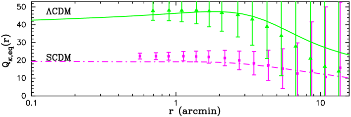
Figure 7: Plots for the SCDM model, as the middle panel in Figure 6. The square symbols show the simulation result for $Q_{\kappa}$ for the SCDM model. The triangles denote the simulation results for the $\Lambda$CDM model, with the error bars scaled to the same area. The comparison shows the sensitivity of $Q_{\kappa}$ to the cosmological model, in particular to $\Omega_{m0}$.

Figure 7 shows a comparison of the halo model prediction for $Q_{\kappa}$ (dot-dashed curve) with simulation results (square symbol) for the SCDM model, as in the middle panel of the previous figure. The halo model prediction matches the simulation results. For comparison, the triangle symbols denote the simulation results for the $\Lambda$CDM model, which shows the strong sensitivity of $Q_{\kappa}$ to the cosmological model, especially to $\Omega_{\rm m0}$.

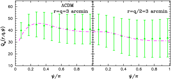
Figure 8: The reduced 3PCF of the convergence field, $Q_{\kappa}$, for the $\Lambda$CDM model against triangle configurations parameterized by $r$, $q$ and $\psi$ (see Figure 4). The left panel shows the result for isosceles triangles with $r=q=3^{\prime}$ fixed and varying $\psi$, while the right panel for more elongated triangles with $r=q/2=3^{\prime}$.

The accuracy of the halo model is further explored in Figure 8, which compares the prediction for the reduced convergence 3PCF, $Q_{\kappa}$, with simulation results against triangle configurations for the $\Lambda$CDM model. Since the halo model employs the spherically symmetric NFW profile, it is interesting to examine whether or not the halo model can properly describe the configuration dependence of the 3PCF seen in simulations which include contributions from realistic aspherical halos with substructure. The left panel shows the result for isosceles triangles with $r=q=3^{\prime}$ against varying the interior angle $\psi$ (see Figure 4 for the triangle geometry). The right panel is for more elongated triangles with $r=2q\approx 3^{\prime}$. Here, the scale $r\approx 3^{\prime}$ is chosen based on the fact that it is in the non-linear regime and unlikely to be affected by the resolution of the simulations. All the plots display excellent agreement between the halo model predictions and the simulations.

4.6 The three-point correlation functions of the shear fields

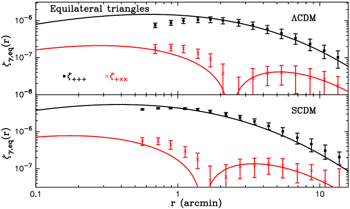
Figure 9: The shear 3PCFs for equilateral triangles against side length $r$ for the $\Lambda$CDM (upper panel) and SCDM (lower panel) models, as in the bottom panel of Figure 6. From symmetry considerations, the four parity-odd functions defined by equation (39) vanish for an $E$-mode, and three of the parity even functions are equal. Hence, only the results for $\zeta_{+++}$ and $\zeta_{+\times\times}$ are shown. Note that the absolute value of $\zeta_{+\times\times}$ is plotted, since it becomes negative at large scales. The two solid curves are the halo model predictions, using only the 1-halo term.

We turn to the shear 3PCFs, which are more complex but are important because they are easier to measure from survey data than the convergence 3PCF. We will focus on the shear 3PCFs rather than the reduced 3PCF, since there is an ambiguity in defining them for the shear. The ambiguity arises from the fact that the $+/\times$ components are defined with respect to the triangle center (see equation (38) to form the 3PCF, hence there is no clear choice for defining the 2PCFs that enter in the denominator of $Q$. One way to do this is to use $\xi_{\gamma,+}$ or $\xi_{\gamma,\times}$ defined with respect to the side of the triangle connecting the two vertices, but we will not pursue this. Figure 9 compares the halo model predictions with simulation results for the shear 3PCFs for equilateral triangles, as in the bottom panel of Figure 6. For equilateral triangles there are only two independent, non-zero 3PCFs: $\zeta_{+++}$ and $\zeta_{+\times\times}=\zeta_{\times+\times}=\zeta_{\times\times+}$, while $\zeta_{\times\times\times}=\zeta_{\times++}=\zeta_{+\times+}=\zeta_{++\times}=0$ (see §3 and also SL03 and TJ03a). The figure thus shows only the results for $\zeta_{+++}$ and $\zeta_{+\times\times}$. The upper and lower panels show the results for the $\Lambda$CDM and SCDM models, as indicated. Note that the plots are on a logarithmic scale and the absolute value of $\zeta_{+\times\times}$ is plotted, since it becomes negative on large scales. The halo model predictions include only the 1-halo contribution. The $\zeta_{+++}$ component carries most of the information of the lensing signal for equilateral triangles (ZS03; TJ03a).

Figure 9 shows that the halo model agrees with the simulation results for angular scales $r\lower 2.15277pt\hbox{$\;\buildrel>\over{\sim}\;$}2^{\prime}$ and $\lower 2.15277pt\hbox{$\;\buildrel>\over{\sim}\;$}1^{\prime}$ for the $\Lambda$CDM and SCDM models, respectively. Whether or not the discrepancy at the smaller scales is genuine is unclear due to the resolution limit of the simulations (see §4.2). We found that the shear correlations are more sensitive to the angular resolution of the simulations than the convergence field. The agreement extends to scales $\lower 2.15277pt\hbox{$\;\buildrel>\over{\sim}\;$}10^{\prime}$, though the PT contribution to the shear 3PCFs is not included, in contrast to the convergence 3PCF where the PT contribution is dominant at $\lower 2.15277pt\hbox{$\;\buildrel>\over{\sim}\;$}5^{\prime}$. This agreement is somewhat surprising, but it might be explained as follows. The spin-2 field properties of the shear fields cause cancellations between the shear 3PCFs to some extent, which explains why the shear 3PCF amplitude is smaller than the convergence 3PCF by an order of magnitude (see Figure 8). The shear 3PCFs appear to be dominated by the coherent shear pattern around a halo rather than filamentary structures in the quasi non-linear regime, which are described by PT (at least for triangles that are close to equilateral).

Both the halo model and the simulations show a flattening and decline in $\zeta_{+++}$ at small scales. The halo model predicts the decline at slightly smaller scales $r\lower 2.15277pt\hbox{$\;\buildrel<\over{\sim}\;$}0.\!\!^{\prime}5$ compared to the simulations. The origin of this feature may be explained as follows. The shear 3PCFs vanish as one goes to zero triangle size (as the three vertices approach the same point), since in this limit it is equivalent to the shear skewness which vanishes from statistical symmetry. This limiting behavior is another way to see why the amplitude of the shear 3PCF is smaller than that of the convergence. Nevertheless, it is possible that the flattening scale of the shear 3PCF reflects a scale related to the size of typical halos that provide the dominant contribution. It will be interesting to study this feature more precisely with higher resolution simulations.

For $\zeta_{+\times\times}$, the agreement between the halo model prediction and the simulation result is not good as for $\zeta_{+++}$. However, the accuracy of the simulation results is likely to be worse because of the smaller amplitude of $\zeta_{+\times\times}$.

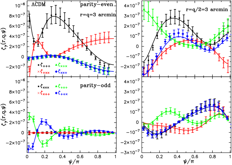
Figure 10: The eight shear 3PCFs for the $\Lambda$CDM model against triangle configurations, as in Figure 8. The upper and lower plots show the results for the parity-even and -odd functions, respectively. Note that range on the y-axis for the right panel is about two times smaller than in the left panel. The solid curves show the halo model predictions for the eight shear 3PCFs, while the symbols are the simulation results as indicated.

The accuracy of the halo model for the shear 3PCFs is tested in greater detail in Figure 10, which compares model predictions with simulations for varying triangle configurations for the $\Lambda$CDM model. The upper and lower panels show the parity-even and -odd functions, respectively. As can be seen from the lower left panel, both the halo model predictions and the simulation results verify that two parity-odd functions vanish: $\zeta_{\times\times\times}=\zeta_{\times++}=0$ for isosceles triangles (see §3). However, the other two parity-odd functions do carry lensing information as pointed out by SL03 (also see TJ03a), as the $\times$ component is at the vertex bounded by unequal sides. For $\psi=\pi/3$ the triangle is equilateral and these two functions also vanish.

The right panel of Figure 10 shows that all the eight functions are non-zero for general triangle configurations (SL03; TJ03a). In contrast to the convergence 3PCF shown in Figure 8, the shear 3PCFs display complex configuration dependences and change sign with varying $\psi$. These features reflect the detailed structure of the underlying mass distribution as well as properties of the spin-2 field generated by an $E$-mode signal. $\zeta_{+++}$ peaks around $\psi=\pi/3$, where the triangle configuration is close to equilateral. For the general triangles shown in the right panel, all the eight functions have roughly comparable amplitude. Comparing the left and right panels shows that more elongated triangles lead to smaller amplitudes of the shear 3PCFs. These results are to be contrasted with the expectation that the 3D mass 3PCF has higher amplitude for elongated triangles on large scales ($\lower 2.15277pt\hbox{$\;\buildrel>\over{\sim}\;$}10$Mpc), reflecting the dominance of anisotropic structures in the perturbative regime (Scoccimarro & Frieman 1999; Bernardeau et al. 2002b; also see Figure 5 in TJ03b). The range $\psi=[0,\pi]$ is shown in our figures; one should keep in mind the relation $\zeta(\psi)=\pm\zeta(2\pi-\psi)$ for the lensing $E$-mode, where $+$ or $-$ sign is taken for the parity-even or -odd functions, respectively (§3; also see Figure 3 in TJ03a ).

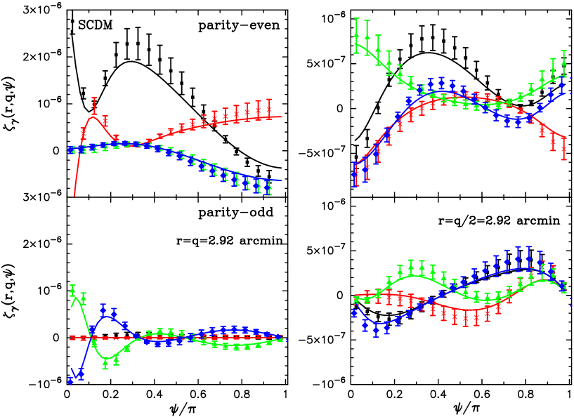
Figure 11: As in the previous figure, for the SCDM model.

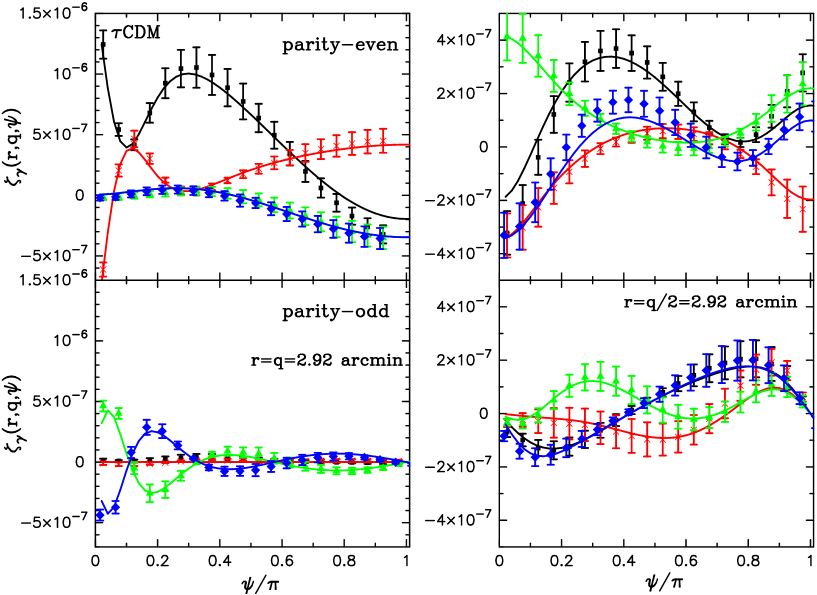
Figure 12: As in the previous figure, for the $\tau$CDM model. The cosmological parameters for the $\tau$CDM model are the same as for the SCDM model, except for the shape parameter $\Gamma$ which is $0.21$, while it is $0.5$ for SCDM.

To further check the accuracy of the halo model for different cosmological models, Figures 11 and 12 show the results for the SCDM and $\tau$CDM models, respectively. Note that the cosmological parameters for the $\tau$CDM model are the same for the SCDM model except for the shape parameter $\Gamma=0.21$ ($\Gamma=0.5$ for the SCDM model). The angular resolution of the two models is the same (Jain et al. 2000). The halo model predictions again match the simulation results for all eight functions. A comparison of Figure 11 and 12 shows that the amplitude of the shear 3PCF depends on the shape of the input linear mass power spectrum. In the context of the halo model picture, this is captured by the dependence of the halo mass function on the power spectrum shape on the angular scales we considered. In summary, from Figures 10-12, one can see that the shear 3PCF amplitudes are sensitive to the cosmological models, but the oscillatory shape of each function is quite similar for the three CDM models.

4.7 Summary: the halo model accuracy for predicting the lensing statistics

Here we summarize the results shown in Figures 5-12, which investigated the 2PCFs and the 3PCFs of the convergence and shear fields. It has been shown that the halo model predictions are in remarkable agreement with the simulation results for all these statistical quantities over the angular scales we have considered. In particular, the halo model reproduces the amplitudes and the complex configuration dependences for the eight shear 3PCFs. We have used only the 1-halo term and not adjusted any model parameters to get this agreement. This implies that the shear 3PCFs result from correlations between the tangential shear pattern around a single NFW profile, as pointed out by TJ03b and ZS03. The agreement is striking, since the halo model rests on simplified assumptions of smooth, spherical halos while the halos in CDM simulations are aspherical and contain substructure (e.g., Jing & Suto 2002). The projection of halos oriented in different directions and the nonlocal properties of the shear appear to dilute the effect of some of the detailed structure of halos and make the spherically symmetric profile a good approximation in the statistical sense.

It is not clear whether the agreement remains on smaller angular scales ($\lower 2.15277pt\hbox{$\;\buildrel<\over{\sim}\;$}1^{\prime}$), due to the resolution limitation of the simulations we have used. It is of great interest to address this issue using higher resolution simulations. On these scales new ingredients may be needed for the halo model as well, such as the inclusion of substructure (Sheth & Jain 2002). The agreement we have shown holds for different cosmological models ($\Lambda$CDM , SCDM and $\tau$CDM models). This implies that the cosmological model dependences can be captured through the spherical collapse model and the mass function used in the halo model. These results lead us to conclude that the halo model provides an analytical method for predicting higher order lensing statistics with sufficient accuracy for our purposes.

5 Measurement of halo profile parameters from shear correlations

In the following we address the question: how can measurements of the lensing 2PCF and 3PCFs be used to constrain halo model parameters? In particular, we focus on the halo profile parameters: the inner slope $\alpha$ for the generalized NFW profile in equation (10) and the halo concentration $c$ in equation (12). We will show that forthcoming lensing surveys can put stringent constraints on these parameters. For this study we will use the convergence 2PCF and 3PCF for simplicity, although the shear correlations are the direct observable. To use the shear 3PCFs, it is necessary to combine all the eight 3PCFs. Since the lensing information obtained combining the eight shear 3PCFs are related to the convergence 3PCF, the results we obtain should hold as a first approximation. We also note that the statistics of the convergence field may be directly measured from future space based surveys such as the one proposed for the SNAP satellite (Jain 2002).

5.1 Sensitivity of the lensing 2PCF and 3PCF to profile parameters

In TJ03b, we showed that the 2PCF and 3PCF of the 3D mass distribution at small scales are sensitive to halo profile parameters (see Figures 12-14 in TJ03b). It was shown that the 3PCF is more sensitive to the halo profile than the 2PCF. This is expected to hold for lensing statistics also, since the lensing fields are projections of the 3D mass distribution.

We derive analytical expressions in Appendix B for the halo convergence for $\alpha=0,1$ and $2$ in the generalized NFW profile of equation (10). To compute the convergence 2PCF and 3PCF for general $\alpha$ ($0\leq\alpha\leq 2$) we simply interpolate from the 1-halo term predictions for $\alpha=0,1$ and $2$, using formulae similar to equation (42) in TJ03b; the interpolation is expected to work to better than $10\%$.

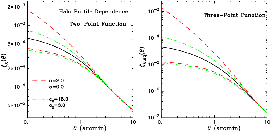
Figure 13: The dependences of the 2PCF (left panel) and 3PCF (right panel) of the convergence field on halo profile parameters. The upper and lower dashed curves show the halo model predictions with $\alpha=2$ and $0$ for the inner slope parameter of the generalized NFW profile of equation (10). The upper and lower dot-dashed curves are the results for the concentration parameter $c_{0}=15$ and $3$. The solid curve is the halo model result for our reference model, the NFW profile with $\alpha=1,c_{0}=9$.

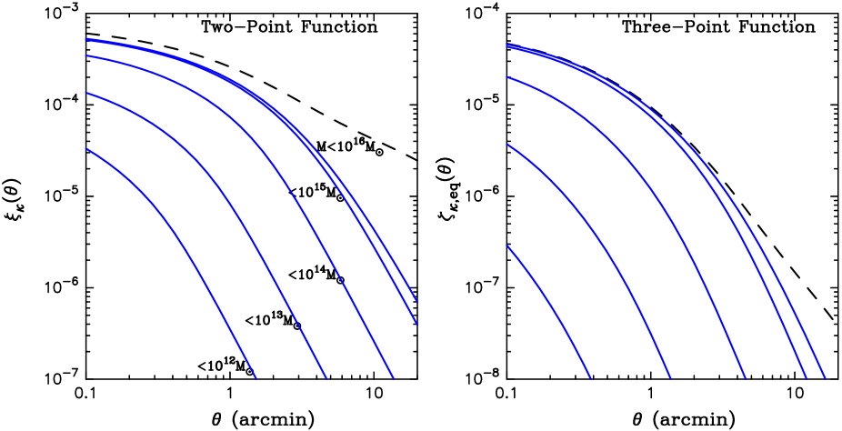
Figure 14: The dependences of the 1-halo term contribution to the convergence 2PCF (left panel) and 3PCF (right panel) on the maximum mass cutoff used in the calculation. From top to bottom, the five solid curves are the results for a maximum mass of $10^{16}$, $10^{15}$, $10^{14}$, $10^{13}$ and $10^{12}M_{\odot}$, as indicated. The dashed curve shows the total halo model prediction. Most contributions arise from halos of $M>10^{13}M_{\odot}$ on the scales we have considered, and the 3PCF is more sensitive to massive halos than the 2PCF.

Figure 13 shows the sensitivity of the convergence 2PCF (left panel) and 3PCF (right panel) to the inner slope parameter $\alpha$ and to the concentration parameter $c_{0}$; in our parameterization $c=c_{0}(1+z)^{-1}(M/M_{\ast})^{-\beta}$ with $\beta=0.13$. Increasing $\alpha$ or $c_{0}$ steepens the 2PCF and 3PCF for scales $\theta\lower 2.15277pt\hbox{$\;\buildrel<\over{\sim}\;$}3^{\prime}$, since it increases the density profile in the inner region, $r\leq r_{\rm vir}/c$. The curves coincide with each other at large scales, because the outer region has the slope $r^{-3}$ for all $\alpha$. The 3PCF is more sensitive to modifications of the halo profile than the 2PCF; this is because of the extra power of the halo profile in the 1-halo term.

Figure 14 shows the mass range of halos that contribute to the lensing statistics on scales of our interest. The figure shows the dependences on the maximum mass cutoff in the halo model calculation on the convergence 2PCF and 3PCF. Massive halos with $M>10^{13}M_{\odot}$ provide more than $80\%$ of the contribution over the scales we have considered. At smaller angular scales, less massive halos are more relevant. One can also see that the 3PCF is more sensitive to massive halos than the 2PCF.

5.2 Covariance of the 2PCF and 3PCF estimators

To rigorously extract parameter information from cosmic shear measurements, it is crucial to consider the covariance between the lensing statistics in different bins. This issue for the shear 2PCFs has been investigated by Schneider et al. (2002b). It was shown that there are strong correlations between the shear 2PCFs in different bins on small scales. Extending their method, we present analytic expressions for the covariance of the convergence 3PCF and 2PCF. Note that the method described below can be extended to compute the covariance for the shear 3PCFs, if one accounts for the spin-2 phase factors of the shear fields and the projection operators.

Following Schneider et al. (2002b), an estimator of the convergence 3PCF from realistic data can be expressed as

$$\zeta^{\rm est}_{\kappa}(r,q,\psi)=\frac{1}{N_{\rm trip}}\sum_{ijk}\kappa_{i}\kappa_{j}\kappa_{k}\Delta_{ijk}(r,q,\psi),\hskip 20.00003ptN_{\rm trip}=\sum_{ijk}\Delta_{ijk}(r,q,\psi),$$ (45)

where index $i$ denotes source galaxies and $N_{\rm trip}$ is the number of triplets of galaxies that form a given triangle configuration within the bin width. The function $\Delta_{ijk}(r,q,\psi)$ is the selection function for triplets: it is unity if the three points with indices $i,j$ and $k$ are in the triangle configuration and zero otherwise. In the weak lensing limit, the observed convergence field can be expressed as the sum of the lensing signal and the noise contamination due to intrinsic ellipticities: $\kappa=\kappa^{\rm lens}+n_{\epsilon}$. The expectation value of the estimator above is obtained by averaging over source ellipticities and performing an ensemble average of the convergence field, denoted by $\langle{\cdots}\rangle$. We will use the notation $\langle{\zeta^{\rm est}_{\kappa}}\rangle\equiv\zeta_{\kappa}$.

The covariance of the convergence 3PCF is defined as

$${\rm Cov}[\zeta_{\kappa},\zeta^{\prime}_{\kappa}]=\langle{(\zeta^{\rm est}_{\kappa}-\zeta_{\kappa})(\zeta^{{\rm est}\prime}_{\kappa}-\zeta_{\kappa}^{\prime})}\rangle=\langle{\zeta^{\rm est}_{\kappa}\zeta^{{\rm est}\prime}_{\kappa}}\rangle-\zeta_{\kappa}\zeta_{\kappa}^{\prime}.$$ (46)

where we have simplified the notation so that $\zeta_{\kappa}$ and $\zeta^{\prime}_{\kappa}$ denote $\zeta_{\kappa}(r,q,\psi)$ and $\zeta_{\kappa}(r^{\prime},q^{\prime},\psi^{\prime})$, respectively. Similarly as done in Schneider et al. (2002b), the first term on the r.h.s. of the above equation can be rewritten as

$$\langle{\zeta_{\kappa}^{\rm est}\zeta^{{\rm est}\prime}_{\kappa}}\rangle=\frac{1}{N_{\rm trip}(r,q,\psi)N_{\rm trip}(r^{\prime},q^{\prime},\psi^{\prime})}\sum_{ijkabc}\Delta_{ijk}(r,q,\psi)\Delta_{abc}(r^{\prime},q^{\prime},\psi^{\prime})\langle{\kappa_{i}\kappa_{j}\kappa_{k}\kappa_{a}\kappa_{b}\kappa_{c}}\rangle.$$ (47)

The covariance estimate thus requires an evaluation of the 6-point correlation function of the observed convergence field. If the noise field and the convergence field are statistically uncorrelated, the 6-point correlation function can be expressed as

$$\langle{\kappa_{i}\kappa_{j}\kappa_{k}\kappa_{a}\kappa_{b}\kappa_{c}}\rangle\approx\sigma_{\epsilon}^{6}(\delta_{ia}\delta_{jb}\delta_{kc}+5~{}{\rm perm.})+\left[\xi_{\kappa}(\theta_{ij})\xi_{\kappa}(\theta_{ka})\xi_{\kappa}(\theta_{bc})+14~{}{\rm perm.}\right],$$ (48)

where $\sigma_{\epsilon}$ is the rms of the intrinsic ellipticities and we have ignored terms of $O(\sigma_{\epsilon}^{4}\xi_{\kappa})$ and $O(\sigma_{\epsilon}^{2}\xi^{2}_{\kappa})$, which are relevant only in the transition regime between those in which the first or second term on the r.h.s of equation (48) dominate. In addition, the second term ignores the non-Gaussian contribution that is due to the connected parts of the three-, four- and six-point correlation functions, and thus underestimates the sample variance. For a more conservative estimate of the non-Gaussian contribution, one might replace the connected parts of the three-, four- and six-point functions with their unconnected parts, providing $\langle{\kappa^{\rm cs}_{i}\cdots\kappa^{\rm cs}_{c}}\rangle=8\left[\xi_{\kappa}(\theta_{ij})\xi_{\kappa}(\theta_{ka})\xi_{\kappa}(\theta_{bc})+14~{}{\rm perms.}\right]$. However, in this paper we use the above equation for simplicity. This is likely to be a good approximation for two reasons. One, our estimates are consistent with the results from simulations which contain the full non-Gaussian contribution, as shown in Figure 15. Moreover the shot noise contribution dominates the covariance on sub-arcminute scales, which provide the main constraints on halo profiles.

Inserting equation (48) into equation (47) and performing an ensemble average over source galaxy positions yields

$${\rm Cov}[\zeta(r,q,\psi),\zeta(r^{\prime},q^{\prime},\psi^{\prime})]=\left[\Delta\zeta_{N}(r,q,\psi)\right]^{2}\delta(\{r,q,\psi\}-\{r^{\prime},q^{\prime},\psi^{\prime}\})+{\cal R}(r,q,\psi,r^{\prime},q^{\prime},\psi^{\prime}),$$ (49)

with

$$\Delta\zeta_{N}(r,q,\psi) \equiv \frac{\sigma_{\epsilon}^{3}}{\sqrt{N_{\rm trip}}}$$ (50)

$$= 2.40\times 10^{-7}\left(\frac{\sigma_{e}}{0.4}\right)^{3}\left(\frac{\Omega_{\rm s}}{10^{3}~{}{\rm deg}^{2}}\right)^{-1/2}\left(\frac{n_{g}}{10^{2}~{}{\rm arcmin}^{-2}}\right)^{-3/2}$$

$$\times\left(\frac{r}{1^{\prime}}\right)^{-1}\left(\frac{\Delta\ln r}{0.1}\right)^{-1/2}\left(\frac{q}{1^{\prime}}\right)^{-1}\left(\frac{\Delta\ln q}{0.1}\right)^{-1/2}\left(\frac{\Delta\psi/\pi}{0.2}\right)^{-1/2},$$

$${\cal R}(r,q,\psi,r^{\prime},q^{\prime},\psi^{\prime}) \equiv \frac{1}{2\pi\Omega_{\rm s}}\int_{0}^{s_{{\rm max}}}\!\!sds\int^{2\pi}_{0}\!d\varphi_{r}\int^{2\pi}_{0}\!d\varphi_{r}^{\prime}\left[\xi(r)\xi(\mbox{{\it\boldmath$s$}}-\mbox{{\it\boldmath$r$}}-\mbox{{\it\boldmath$q$}})\xi(\mbox{{\it\boldmath$q$}}^{\prime})+\mbox{ 14 perms.}\right](s,\varphi_{r},\varphi_{r}^{\prime};r,q,\psi,r^{\prime},q^{\prime},\psi^{\prime}),$$ (51)

where $\Omega_{\rm s}$ and $n_{g}$ are the survey area and the number density of source galaxies, respectively, and $\Delta r$, $\Delta q$ and $\Delta\psi$ denote the bin widths for the three parameters $(r,q,\psi)$ that specify the triangle configuration. The notation used in equation (51) is $s_{\rm max}=\sqrt{\Omega_{\rm s}/\pi}$, $\mbox{{\it\boldmath$r$}}=r(\cos\varphi_{r},\sin\varphi_{r})$, $\mbox{{\it\boldmath$q$}}=q(-\cos(\psi-\varphi_{r}),\sin(\psi-\varphi_{r}))$ and so on. We have assumed that the survey geometry does not affect covariance estimation – a good approximation as long as we consider sufficiently small scales compared to the survey size. The first term on the r.h.s of equation (49) denotes the shot noise contribution due to the intrinsic ellipticities, where the function $\delta(\{r,q,\psi\}-\{r^{\prime},q^{\prime},\psi^{\prime}\})$ is defined to be unity if $r=r^{\prime}$, $q=q^{\prime}$ and $\psi=\psi^{\prime}$ within the bin widths, and zero otherwise. The derivation of this term requires an estimate of the triplet number for a given triangle configuration, which we estimate as $N_{\rm trip}=n_{g}\Omega_{\rm s}\times n_{g}\pi r(\Delta r)\times n_{g}q(\Delta q)(\Delta\psi)$, where the first, second and third factors denote the number of galaxies at the vertices, 1, 2 and 3, respectively (see §4.3). The second term ${\cal R}$ in equation (49) denotes the sample variance. Several interesting points made by Schneider et al. (2002b) for the 2PCF hold for the convergence 3PCF as well. (1) All the terms are proportional to $\Omega_{\rm s}^{-1}$, and therefore the relative contribution of the terms is independent of survey area, if the area is sufficiently large. (2) The sample variance ${\cal R}$ does not depend on the survey particulars such as $n_{g}$ and $\sigma_{\epsilon}$. Further, ${\cal R}$ is independent of the bin widths. This implies that combining the 3PCFs in different bins cannot reduce the sample variance. This is indeed verified by ray-tracing simulations. (3) The off-diagonal components of the covariance arise only from the sample variance ${\cal R}$.

To compute the sample variance ${\cal R}$ for a given cosmological model using equation (49), we first make a table of the model predictions of the convergence 2PCF as a function of the separation angle. Then, we can use the same table to compute the sample variance between the two convergence 3PCFs of any triangle configurations. Therefore, this method is much more tractable than a direct implementation including contributions from the three-, four- and six-point functions, where we have to account for their configuration dependences in the integration of equation (51). An alternative way to estimate the covariance is to use ray-tracing simulations. However, to do this rigorously requires an adequate number of independent realizations, since sample variance is large for the higher-order moments. The PTHalos method recently proposed by Scoccimarro & Sheth (2002) can be a powerful tool for such an approach.

Likewise, we can derive the covariance of the convergence 2PCF as

$${\rm Cov}[\xi(r),\xi(r^{\prime})]=[\Delta\xi_{N}(r)]^{2}\delta(r-r^{\prime})+{\cal R}_{\rm 2pt}(r,r^{\prime})$$ (52)

with

$$\Delta\xi_{N} \equiv \frac{\sigma^{2}_{\epsilon}}{\sqrt{N_{\rm pair}}}=1.5\times 10^{-6}\left(\frac{\sigma_{e}}{0.4}\right)^{2}\left(\frac{\Omega_{\rm s}}{10^{3}~{}{\rm deg}^{2}}\right)^{-1/2}\left(\frac{n_{g}}{10^{2}~{}{\rm arcmin}^{-2}}\right)^{-1}\left(\frac{r}{1^{\prime}}\right)^{-1}\left(\frac{\Delta\ln r}{0.1}\right)^{-1/2},$$ (53)

$${\cal R}_{\rm 2pt}(r,r^{\prime}) \equiv \frac{1}{2\pi\Omega_{\rm s}}\int_{0}^{s_{\rm max}}\!\!sds\int^{2\pi}_{0}\!\!d\varphi_{r}\int^{2\pi}_{0}\!\!d\varphi_{r}^{\prime}\left[\xi(\mbox{{\it\boldmath$s$}})\xi(|\mbox{{\it\boldmath$s$}}+\mbox{{\it\boldmath$r$}}^{\prime}-\mbox{{\it\boldmath$r$}}|)+\xi(|\mbox{{\it\boldmath$s$}}+\mbox{{\it\boldmath$r$}}^{\prime}|)\xi(|\mbox{{\it\boldmath$s$}}-\mbox{{\it\boldmath$r$}}|)\right],$$ (54)

where the number of pairs are estimated as $N_{\rm pair}=n_{g}\Omega_{\rm s}\times n_{g}\pi r(\Delta r)$.

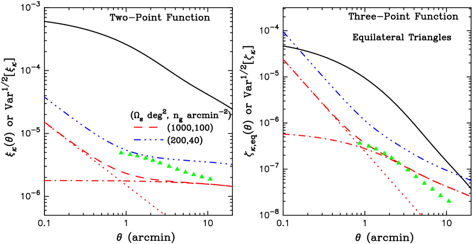
Figure 15: Error estimates for measurements of the convergence 2PCF (left panel) and 3PCF (right panel) for the $\Lambda$CDM model. The error estimate includes both the shot noise due to intrinsic ellipticities, with rms $\sigma_{\epsilon}=0.4$, and sample variance. Two cases for survey area $\Omega_{\rm s}$ and number density of source galaxies $n_{g}$ are shown. For $(\Omega_{\rm s},n_{g})=(1000~{}{\rm deg}^{2},100~{}{\rm arcmin}^{-2})$, the dotted and dot-dashed curves show the shot noise contribution and the sample variance separately: shot-noise dominates on sub-arcminute scales. The solid curve shows the halo model prediction for the 2PCF or the 3PCF. The triangular symbols show the sample variance estimated from simulations for $\Omega_{\rm s}=1000$.

Figure 15 plots the square root of the diagonal component of the covariance matrix for the convergence 2PCF (left panel) and 3PCF (right panel) for the $\Lambda$CDM model. This is an estimate of the error on the 2PCF and 3PCF measurements from a lensing survey. We consider two cases, specified by the survey area $\Omega_{\rm s}$ and the number density of source galaxies $n_{g}$. The dashed and broken curves show the results for $(\Omega_{s},n_{g})=(1000,100)$ and $(200,40)$ in units of ${\rm degree}^{2}$ and ${\rm arcmin}^{-2}$, respectively. The former is expected from future imaging survey, while the latter applies for a survey like the CFHT Legacy Survey, which has just begun. For $(\Omega_{s},n_{g})=(1000,100)$, the dotted and dot-dashed curves show the shot noise contamination and the sample variance separately, implying that the shot noise provides the dominant contribution at small scales $\lower 2.15277pt\hbox{$\;\buildrel<\over{\sim}\;$}1^{\prime}$. The triangle symbols denotes the simulation results for the sample variance for $\Omega_{\rm s}=1000$ degree². Note that the simulation result is computed from 36 realizations of a 11.7 degree² simulated map, and is then scaled as $\propto\Omega_{\rm s}^{-1/2}$. Out analytic estimates are consistent with the simulation results, within the rather large error bars of the latter (not plotted to preserve clarity).

The solid curve in each panel of Figure 15 shows the halo model prediction for the 2PCF or the 3PCF. Comparing the solid curves with the error estimate gives the signal-to-noise ($S/N$) ratio for measuring the 2PCF and 3PCF. Clearly these survey parameters will allow for measurements of shear correlations at high significance, even on sub-arcminute scales. We note that the $S/N$ estimate for the 3PCF is only for one triangle configuration – we can combine the 3PCFs from different configurations to improve the $S/N$ at these scales.

5.3 Constraints on $\alpha$ and $c_{0}$

Next we apply the covariances computed above to demonstrate how combined measurements of the 2PCF and 3PCF can be used to constrain parameters of the halo profile. We use the standard $\chi^{2}$ statistic, expressed for our case as:

$$\chi^{2}=\chi_{\rm 2pt}^{2}+\chi_{\rm 3pt}^{2},$$ (55)

where

$$\chi^{2}_{\rm 2pt} \equiv \sum_{i\leq j}(\hat{\xi}_{i}-\xi_{i})[{\rm Cov}(\xi)]^{-1}_{ij}(\hat{\xi}_{j}-\xi_{j}),$$

$$\chi^{2}_{\rm 3pt} \equiv \sum_{i\leq j}(\hat{\zeta}_{i}-\zeta_{i})[{\rm Cov}(\zeta)]^{-1}_{ij}(\hat{\zeta}_{j}-\zeta_{j}),$$ (56)

where $\hat{\xi}$ and $\hat{\zeta}$ denote the 2PCF and 3PCF for the fiducial model and $[{\rm Cov}]^{-1}_{ij}$ denotes the inverse of the covariance matrix. The index $i$ runs among different bins for $\xi$ and $\zeta$. In equation (55), we have ignored the covariance between the 2PCF and 3PCF for simplicity. We make this approximation because only the sample variance contributes to this covariance (the shot noise contribution vanishes as it involves the fifth power of the intrinsic ellipticities), which is small on sub-arcminute scales as discussed above.

So far we have used the parameters $r$, $q$ and $\psi$ to describe triangle configurations. To perform the $\chi^{2}$ fitting we employ an alternative set of parameters used in the literature (e.g., Peebles 1980):

$$r\equiv\theta_{12},\hskip 20.00003ptu\equiv\frac{\theta_{23}}{\theta_{12}},\hskip 20.00003ptv\equiv\frac{\theta_{31}-\theta_{23}}{\theta_{12}},$$ (57)

with the condition $\theta_{12}\leq\theta_{23}\leq\theta_{31}$, which imposes the constraints $u\geq 1$ and $0\leq v\leq 1$. Different sets of $r$, $u$ and $v$ correspond to different triangles, so we do not have to worry about double-counting.

We treat the inner slope parameter $\alpha$ and the halo concentration normalization $c_{0}$ as free parameters. We fix $\beta=0.13$ (the mass dependence of the concentration) and we set the other model parameters to be those for the $\Lambda$CDM model. We discuss below why this choice is a good first attempt at the use of correlation statistics to measure halo profiles. As shown in Figure 13, these profile parameters are sensitive to the lensing statistics at small scales $\lower 2.15277pt\hbox{$\;\buildrel<\over{\sim}\;$}2^{\prime}$. We therefore restrict ourselves to these scales. We consider 10 logarithmic bins in $r=[0.\!\!^{\prime}12,2^{\prime}]$ with the bin width $\Delta r/r=0.1$. For the 3PCF, we consider 5 bins each for $u$ and $v$: $u=1,2,3,4,5$ and $v=0.1,0.3,0.5,0.7,0.9$. Thus we use 10 bins for the 2PCFs and 250 for the 3PCF. How the binning affects the fitting of model parameters must be carefully examined, to avoid over- or under-estimating the constraints (e.g, Scoccimarro & Frieman 1999). Since we correctly take into account the covariance for the 2PCF and 3PCF, including the off-diagonal components, we avoid over-constraining the parameters. The triplet number used for the shot noise evaluation is estimated for the binning we consider as $N_{\rm trip}=n_{g}^{3}\Omega_{\rm s}\times\pi r\Delta r\times qr\Delta u\Delta v$ with $\Delta u=1$ and $\Delta v=0.2$. To save computational expense for the sample variance of the 3PCF, we ignore the dependence on the $v$ parameter – we compute the sample variance for different bins of $r$ and $u$, but with $v=0.5$ fixed, resulting in $50\times 50$ computations for the sample variance. This is adequate, since the configuration dependence is weak as shown in Figure 8.

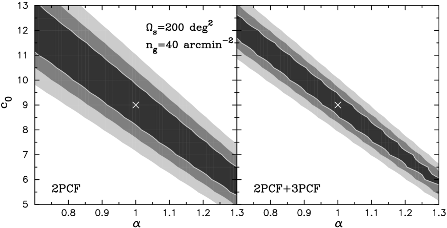
Figure 16: Contour plots of the constraints on the inner slope parameter $\alpha$ and the halo concentration $c_{0}$ expected from a survey with area $\Omega_{\rm s}=200$ degree² and $n_{g}=40$ arcmin^-2. The left panel shows the result if we use only the 2PCF measurement, while the right panel shows the result from combined measurements of the 2PCF and 3PCF. The cross symbol denotes input fiducial model of $(\alpha,c_{0})=(1.0,9.0)$. To perform the fitting, we have used measurements on scales $[0.\!\!^{\prime}2,2^{\prime}]$ and combined $250$ triangle configurations for the 3PCF (see text for details). The three shaded regions represent $\Delta\chi^{2}=2.30(68.3\%)$, $6.17(95.4\%)$ and $11.8(99.7\%)$, respectively. The 3PCF measurement can tighten the constraints, reflecting the fact that it carries lensing information complementary to the 2PCF.

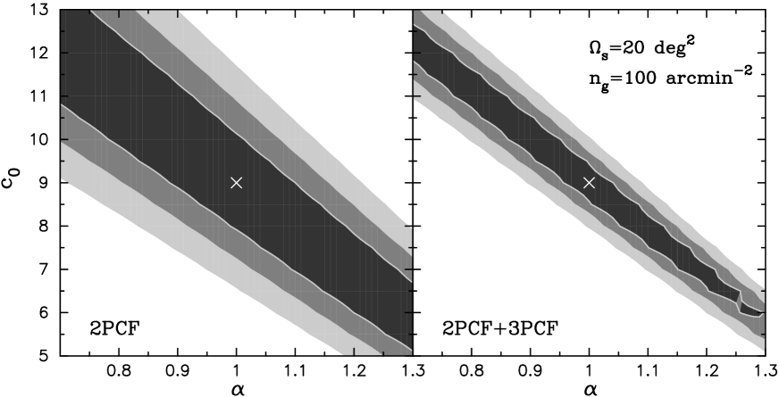
Figure 17: As in the previous figure, but for a survey with $\Omega_{\rm s}=20$ degree² and $n_{g}=100$ arcmin^-2. The results show the value of increased number density of galaxies that can be achieved with a deeper survey. For such a survey the 3PCF provides a much larger improvement in the constraints.

Figure 16 shows contour plots of the constraints on the inner slope parameter $\alpha$ and the halo concentration $c_{0}$. We consider $\Omega_{\rm s}=200$ degree² and $n_{g}=40$ arcmin^-2 for the survey area and the number density of source galaxies, respectively. The left panel shows the constraints if we use the measurement of the 2PCF only, while the right panel shows the constraints from combined measurements of the 2PCF and the 3PCF. The cross symbol denotes our fiducial model of $(\alpha,c_{0})=(1,9)$, which is the NFW profile with the concentration given by Bullock et al. (2001). For a Gaussian probability distribution function for the 2PCF and 3PCF, the three shaded regions correspond to $\Delta\chi^{2}=2.30$, $6.17$ and $11.8$ corresponding to $68.3\%$, $95.4\%$ and $99.73\%$ confidence levels (C.L.), respectively. One can see that the constraints on $\alpha$ and $c_{0}$ are degenerate: the effect of increasing (decreasing) $\alpha$ on the 2PCF and 3PCF is compensated by decreasing (increasing) $c_{0}$. Nevertheless, the right panel shows that the 3PCF measurement can tighten the constraints, implying that the 3PCF provides additional information on these parameters, although the parameter degeneracy is not broken. As a result, this type of survey can be used to put stringent constraints on $\alpha$ and $c_{0}$ within $5\%$ level ($95\%$ C.L.), if one of the parameters is fixed, and systematic uncertainties in the measurements and the theoretical model do not dominate.

Figure 17 shows the result expected from a different type of survey from the one in the previous figure: a deep, small area survey, with $(\Omega_{\rm s},n_{g})=(20,100)$. For this case, the 3PCF can substantially tighten the constraints provided from the 2PCF. However, the degeneracy between $\alpha$ and $c_{0}$ remains. Recently, Takada & Hamana (2003) proposed that a joint measurement of the magnification statistics and the cosmic shear could be used to break the degeneracy or at least put upper bounds on $\alpha$ and $c_{0}$, since the amplitude of the magnification correlation is more sensitive to an increase of $\alpha$ and $c_{0}$ than the cosmic shear correlation. This arises from the non-linear relation between the magnification and shear, given by $\mu=|(1-\kappa)^{2}-\gamma^{2}|^{-1}$.

6 Discussion

In this paper, we have developed the halo model for computing the higher order correlations of the cosmic shear field, extending the real-space dark matter halo approach developed in TJ03b. A detailed investigation of the three-point correlation functions (3PCF) of the convergence and shear fields with respect to the size and configuration dependence of triangles has been presented. Our method provides an accurate, analytical way of computing the 3PCFs with little computational expense. We have focused on the eight shear 3PCFs defined from combination of the $+/\times$ projections of the shear fields at each vertex of a given triangle (SL03, ZS03 and TJ03a). The shear 3PCFs defined in this way have characteristic properties that help disentangle the lensing $E$-mode from the the $B$-mode due to possible systematic errors and other non-linear effects (see §3). They are a direct probe of the gravitational clustering of the mass distribution and can provide an independent test of the CDM paradigm of structure formation.

We have carefully checked the accuracy of our model by comparing the predictions with ray-tracing simulation results. We paid particular attention to the triangle configuration dependences of the 3PCFs, since our halo model uses simple spherically symmetric profiles. We find excellent agreement over the angular scales and models we have considered, as shown in Figures 5-12. The halo model reproduces the complex configuration dependences for the eight shear 3PCFs, as well as their amplitudes. The agreement is found for plausible model ingredients: mass function (Sheth & Tormen 1999) and NFW halo profiles with recent prescriptions for the halo concentration (Bullock et al. 2001). We chose the best parameter values identified in the literature and did not adjust any parameters.

On scales $\lower 2.15277pt\hbox{$\;\buildrel>\over{\sim}\;$}1^{\prime}$ the 3PCF can be used to break degeneracies in cosmological parameters, in particular in the $\sigma_{8}$-$\Omega_{\rm m0}$ determinations so far made from the 2PCF measurement. Figures 6-12 show a clear dependence of the lensing 3PCFs on the cosmological models. In addition, on large scales the 3PCF can constrain primordial non-Gaussianity, which can be separated from the gravitationally induced signal using its dependence on scale (R. Scoccimarro, private communication). In practice, measuring the shear 3PCFs is more feasible than the convergence 3PCF, since obtaining the convergence requires a non-local reconstruction from the observed shear field. Detections of shear three-point moments have recently been reported (Bernardeau et al. 2002a; Pen et al. 2003). Thus, current survey data are likely to already allow for shear 3PCF measurements (see Figure 15 and Figure 4 in TJ03a for theoretical justification). Our method provides the only well-tested analytical approach to interpret the measured signals in terms of cosmological parameters.

A second application we have proposed is to use shear statistics on sub-arcminute scales to constrain halo profile properties. Forthcoming lensing surveys promise to measure the sub-arcminute signals with high significance (see Figure 15; also see Figures 17 and 18 in Van Waerbeke et al. 2001b for a measurement of the shear 2PCFs). This will open a new window in the use of shear correlation functions, beyond the determination of cosmological parameters. The $n$-point correlation functions on sub-arcminute scales arise mainly from correlations between the lensing fields around a single halo of $M>10^{13}M_{\odot}$ (see Figure 14). The halo model allows us to interpret the measured signals in terms of the halo profile properties. The inner slope of the generalized NFW profile and the halo concentration are sensitive to the amplitudes of the lensing 2PCF and 3PCF on these scales (see Figure 13).

We have demonstrated how combined measurements of the 2PCF and 3PCF can put stringent constraints on halo profile properties from forthcoming lensing data. This was done by taking into account the covariance for the 2PCF and 3PCF measurements, which contains contributions from the shot noise due to the intrinsic ellipticities and sample variance. For example, Figure 16 shows that a survey with parameters similar to those of the CFHT Legacy survey can constrain the inner slope parameter with $5\%$ accuracy ($95\%$ C.L.) if the halo concentration is fixed. Figure 17 shows the dramatic improvements possible with a deeper survey; on the basis of these figures, it follows that a deep survey with area $\lower 2.15277pt\hbox{$\;\buildrel>\over{\sim}\;$}200$ square degrees and source number density $\sim 100$ per square arcminutes can achieve an accuracy of $1\%$ in density profile parameters. The use of the 3PCF is critical in being able to achieve this accuracy, and the use of the four-point function would also be valuable if it could be measured. In this paper we have ignored the effect of uncertainties in the mass function and its possible degeneracy with the inner slope and concentration. White (2002) suggested adjustments to the parameters in the Sheth-Tormen mass function from fitting to simulations. We confirmed that this modification alters the halo model predictions for lensing correlations over angular scales ($\lower 2.15277pt\hbox{$\;\buildrel<\over{\sim}\;$}5^{\prime}$) where the 1-halo term is relevant. Therefore, measuring the lensing 2PCF and 3PCF can be similarly used to constrain the shape of halo mass function over a mass range of $10^{13}-10^{15}M_{\odot}$. This would be complementary to other methods such as cluster counts. Breaking the degeneracy in the halo model parameters will require either using the different 3PCFs of the shear, which we have not done here, or input from other methods such as the convergence reconstruction approach discussed below, or a statistical study of strong lensing, $X$-ray and SZ effect on cluster/group scales. These are important issues to be addressed.

A fundamental result from CDM simulations is that the density profiles of halos are universal across a wide range of mass scales (e.g., NFW). Therefore, applying our method to different length scales would sample halo profiles on different mass scales and offer a powerful test of the CDM paradigm. The halo model formalism can also be extended to include the effects of substructure, currently a subject of study due to a possible conflict between CDM theory and observations (e.g. Sheth & Jain 2002; Dalal & Kochanek 2002). Substructure and triaxiality of halos, discussed further below, would increase the amplitude of correlation functions on the smallest scales. Since the two-, three-, and four-point functions scale differently with these effects, a careful study is merited to develop the correlation function approach as a probe of different small scale effects. Using lensing correlations on scales of $0.1-2$ arcminutes, halos with masses of $10^{13}-M^{15}M_{\odot}$ will be probed.

The method of constraining halo profile properties from shear correlations is complementary to the approaches of Reblinsky & Bartelmann (1999), Dahle, Hannested & Sommer-Larsen (2003), White et al. (2002), Miyazaki et al. (2002) and Padmanabhan et al. (2003). They rely on the reconstruction of the convergence field from observed ellipticities (see Dahle et al. 2003 and Miyazaki et al. 2002 for the implementation to actual data). Halo profiles are constrained by looking at convergence profiles around individual peaks in the convergence map. However, there are some limitations to this method. The first is lensing projection effects – we cannot accurately measure properties of the primary halo due to superposition with a void region or less massive halos along the same line of sight, even if the redshift of the lens halo is available (White et al. 2002; Padmanabhan et al. 2003). The other limitation is the angular resolution of the convergence reconstruction. In practice, reconstructing the convergence field on a given patch of the sky requires an averaging of the observed ellipticities over an adequate number of source galaxies to reduce the noise contamination as well as enhance the contrast of the signals arising from halos. For plausible survey parameters the reconstruction resolution is larger than an arcminute. The reconstructed convergence around a halo is thus smoothed, which makes it difficult to see the inner region in the halo profile. Padmanabhan et al. (2003) concluded that the inner slope of NFW profiles cannot be constrained using convergence maps.

The resolution limitation of convergence maps can be offset by stacking clusters and by follow-up deeper weak lensing observations and other methods such as the SZ effect, $X$-ray observations and strong lensing. It is not an easy task however, and is subject to biases associated with identifying centers and mass scales with peaks. The strength of the correlation function method we have discussed is that it allows for constraints on the inner halo profile statistically, even though individual halos are not resolved on these scales. Our approach treats the data objectively, while taking a parameterized approach to the modeling. This appears a sensible approach at a time when cosmological parameters are well constrained and we have a broad understanding of halo properties.

The real-space halo model formulation, developed in TJ03b and this paper, does not rely on a model of the 3D non-linear power spectrum. This fact leads to interesting applications for lensing statistics. We can directly compute any $n$-point correlation functions of lensing observables, such as the reduced shear field $g=\gamma/(1-\kappa)$ and the lensing magnification $\mu=1/[(1-\kappa)^{2}+\gamma^{2}]$ (Takada & Hamana 2003). This can be done merely by replacing $\gamma_{M}$ in equation (24) with $g_{M}$ or $\mu_{M}$ for a given halo of mass $M$, respectively. The resulting prediction is exact in the sense that it fully accounts for the non-linear contribution of lensing. So far, the cosmological interpretation of lensing two-point statistics has been made using theoretical predictions computed from a model of the 3D power spectrum, which requires a perturbative approach, such as setting $\mbox{{\it\boldmath$g$}}\approx\mbox{{\it\boldmath$\gamma$}}$ or $\mu\approx 1+2\kappa$ (e.g., Van Waerbeke et al. 2001b; McKay et al. 2001; Guzik & Seljak 2002; Benitez & Martinez-Gonzalez 1997; Gaztañaga 2003).

There are some uncertainties we have ignored in the halo model formulation. We have employed a spherically symmetric halo profile, while CDM simulations show that halos are triaxial (Jing & Suto 2002). In addition, high-resolution simulations have also shown that about $10\%$ of mass distribution in a halo is in small sub-clumps (e.g, Ghigna et al. 2000). We have shown that the halo model computed from the NFW profile matches the simulation results for all the lensing statistics we have considered. However, it is unclear whether this agreement holds on sub-arcminute scales. The 3PCF can be the lowest order statistical quantity to probe the detailed mass distribution of halos via its dependence on triangle configurations. Substructure and triaxiality are expected to have different scale and configuration dependences than changes to the halo parameters that we have considered. It is an interesting problem for future work to work out in detail the different effects that emerge on scales of order $\sim 0.1$ arcminute. For the applications described above, it is important to test the analytical predictions with ray-tracing simulation with higher resolution. This is a pressing need and a challenge for future numerical work. The PTHalos method developed by Scoccimarro & Sheth (2002) could be a powerful alternate tool for such a study.

We would like to thank T. Hamana for kindly providing his ray-tracing simulation data and for discussions. We also thank R. Scoccimarro, R. Sheth, M. Jarvis and G. Bernstein for valuable comments and discussions and thank P. Schneider for valuable discussions on the parity transformation properties of the shear three-point functions. This work is supported by NASA grants NAG5-10923, NAG5-10924 and a Keck foundation grant.

Appendix A Validity of the real-space halo approach for shear statistics

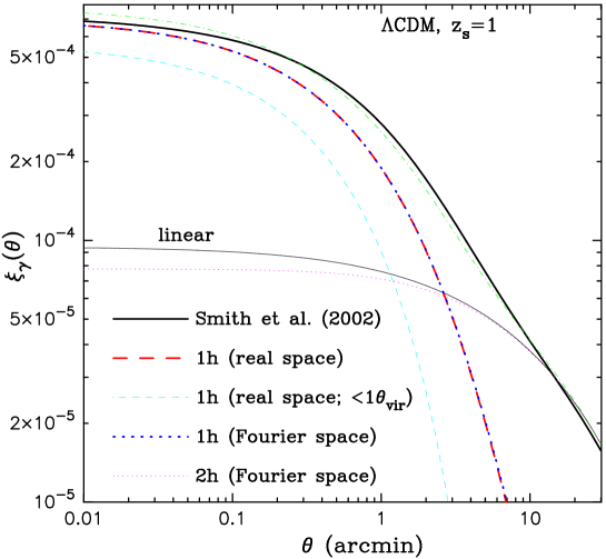
Figure 18: The two-point correlation function of the shear field, $\xi_{\gamma}(\theta)=\langle{\mbox{{\it\boldmath$\gamma$}}\cdot\mbox{{\it\boldmath$\gamma$}}^{\ast}}\rangle$, vs. separation angle $\theta$. The thick dashed curve shows the real-space halo model prediction for the 1-halo term, computed using equation (24), while the thick dotted curve shows the Fourier-space halo model prediction. The sum with the 2-halo term, denoted by the thin dotted curve, leads to the halo model prediction for the total power (1h+2h terms) shown by the dot-dashed curve. For comparison, the thick and thin solid curves show the predictions computed from the Smith02 fitting formula for the non-linear mass power spectrum and the linear power spectrum, respectively. The thin dashed curve is the real-space halo model prediction when the integration range is confined to the virial radius.

In this appendix, we address the validity of the real-space halo model developed in §2.4.

Figure 18 plots the shear 2PCF, $\xi_{\gamma}(\theta)=\langle{\mbox{{\it\boldmath$\gamma$}}\cdot\mbox{{\it\boldmath$\gamma$}}^{\ast}}\rangle$, against separation angle $\theta$ for the $\Lambda$CDM model and source redshift $z_{s}=1$. The thick dashed and dotted curves are the real-space and Fourier-space halo model predictions for the 1-halo term, which are computed using equations (24) and (31), respectively. Note that we have used the NFW profile. There is excellent agreement over the angular scales we have considered, verifying that the real-space model formulated in §2 is equivalent to the Fourier-space model. This agreement is quite encouraging, since the real-space halo model for the shear field contains an infinite integration range to account for the non-local property of the shear fields. To more explicitly demonstrate the importance of the integration range, the thin dashed curve is the real-space halo model prediction when the integration range $\int\!\!d^{2}\mbox{{\it\boldmath$s$}}$ is confined to the virial region, as is done for the convergence field (see equations (23)). It significantly underestimates the 1-halo term. Figure 3 in TJ03b also demonstrates that the real-space halo model for the convergence field is equivalent to the Fourier-space halo model. These results lead us to conclude that the real-space halo model formulation for the shear and convergence fields has been made in a self-consistent way, in agreement with the Fourier-space model well studied in the literature (e.g., Cooray & Sheth 2002).

The thin dotted curve denotes the 2-halo term, which provides the dominant contribution to the 2PCF for $\theta\lower 2.15277pt\hbox{$\;\buildrel>\over{\sim}\;$}4^{\prime}$. For comparison, the thin solid curve is the result for $\xi_{\gamma}$ computed from the linear mass power spectrum. It very slightly overestimates the 2-halo term which includes the biasing of halos. The 2-halo term thus captures the clustering properties in the linear regime.

The accuracy of the halo model for predicting the lensing 2PCFs can be seen by comparing the dot-dashed and thick solid curves (the detailed comparison with ray-tracing simulation results will be presented below). The dot-dashed curve shows the total halo model prediction (1- plus 2-halo terms), while the thick solid curve is the result computed from the fitting formula proposed in Smith et al. (2002) (hereafter Smith02). The Smith02 formula was calibrated to reproduce the non-linear mass power spectra from high resolution $N$-body simulations for various cosmological models. As can be seen, the halo model prediction matches the Smith02 result within $10\%$ at $0.\!\!^{\prime}1\leq\theta\leq 30^{\prime}$. The reliable range of the Smith02 formula, is $k\lower 2.15277pt\hbox{$\;\buildrel<\over{\sim}\;$}10~{}h\mbox{Mpc}^{-1}$ in the mass power spectrum. Since the lensing field is the projected field of the 3D mass distribution, the valid range roughly corresponds to the angular scale $\theta\lower 2.15277pt\hbox{$\;\buildrel>\over{\sim}\;$}2\pi/[k_{\rm max}d_{A}(z=0.4)]\approx 0^{\prime}\!\!.6$, where $z=0.4$ is close to the peak redshift of the lensing projection function for the source redshift $z_{s}=1$ (e.g., see Figure 4 in TJ02). Therefore, it is unclear whether or not the discrepancy between the halo model and the Smith02 result at $\theta\lower 2.15277pt\hbox{$\;\buildrel<\over{\sim}\;$}0.\!\!^{\prime}1$ is genuine.

It is worth mentioning why we use the fiducial model $(c_{0},\beta)=(9,0.13)$ for the halo concentration in this paper, since we used a steeper mass slope $\beta=0.2$ in TJ02 and TJ03b. The Smith02 formula predicts a steeper $k$ slope of the non-linear power spectrum $P(k)$ than predicted from the fitting formula of Peacock & Dodds (1996) (hereafter PD), which has been widely used in the literature. For the halo model, the $k$-slope is determined by the halo profile parameters, the slope of the mass function, and the input linear power spectrum (Seljak 2000; Ma & Fry 2000a,b,c; TJ03b). The halo model with $\beta=0.13$ gives a slightly better fit to the $k$-slope of the Smith02 power spectrum than with $\beta=0.2$. It is reassuring that we find agreement with N-body simulations with plausible ingredients for the halo model, each of which is supported by independent studies: the halo profile (NFW), the halo concentration (Bullock et al. 2001) and the halo mass function (Sheth & Tormen 1999). These studies explored halo properties by resimulating regions containing halos in a larger scale simulation with a higher resolution simulation. Hence, one advantage of the halo model is that it can be easily refined by incorporating results from different $N$-body simulations with different sizes.

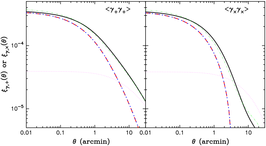
Figure 19: The two-point correlation functions of the shear fields, $\xi_{\gamma,+}$ (left panel) and $\xi_{\gamma,\times}$ (right panel), as in Figure 18. Although the 2-halo term for $\xi_{\gamma,\times}$ overestimates the amplitude at large scales $\theta\lower 2.15277pt\hbox{$\;\buildrel>\over{\sim}\;$}5^{\prime}$, the halo model reproduces the Smith02 result because the 1-halo term is negative.

Figure 19 compares the theoretical predictions for $\xi_{\gamma,+}(\theta)$ (left panel) and $\xi_{\times}(\theta)$ (right panel), as done in the previous figure. The real-space halo model result for the 1-halo term (thick dashed curve) again agrees with the Fourier-space result (thick dotted curve) for both $\xi_{\gamma,+}$ and $\xi_{\gamma,\times}$. The agreement is as a result of the integration of the phase factors $\epsilon_{\mu}\epsilon_{\nu}$ in equation (25) for the real-space case. Comparison of the dot-dashed curve with the solid curve in each panel shows that the halo model prediction for the total 2PCF matches the Smith02 result. Note that, although the 2-halo term (or the linear theory prediction) for $\xi_{\gamma,\times}$ overestimates the amplitude at large scales $\theta\lower 2.15277pt\hbox{$\;\buildrel>\over{\sim}\;$}5^{\prime}$, the agreement of the halo model with the Smith02 result at these scales results from sum of the negative 1-halo term plus the 2-halo term.

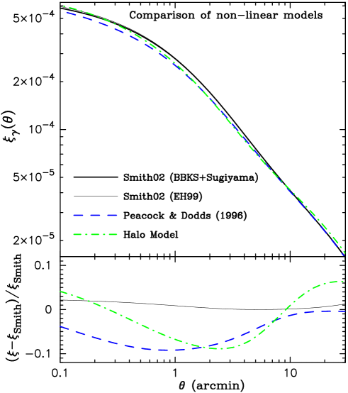
Figure 20: Comparison of model predictions for $\xi_{\gamma}$. The solid, dashed and dot-dashed curves are the results from the Smith02 formula, the PD formula and the halo model, respectively. The lower panel explicitly shows the deviation of each model prediction from the Smith02 model. Although all the results agree with each other within $10\%$, the Smith02 result for $\xi_{\gamma}$ is higher than the PD result by $0-10\%$ at $0^{\prime}\!\!.1\lower 2.15277pt\hbox{$\;\buildrel<\over{\sim}\;$}\theta\lower 2.15277pt\hbox{$\;\buildrel<\over{\sim}\;$}10^{\prime}$ (see text for details). Note that the Smith02 result is computed using the BBKS transfer function. To demonstrate the effect of the input linear power spectrum, the thin solid curve is the Smith02 result when we use the fitting formula of Eisenstein & Hu (1999), which is more accurate.

Figure 20 compares theoretical predictions for $\xi_{\gamma}$ from various models of non-linear gravitational clustering. The thick solid, dashed and dot-dashed curves are the results from the Smith02 formula, the PD formula and the halo model, respectively. The lower panel shows the deviation relative to the Smith02 result (thick solid curve) and shows agreement among these models within 10$\%$ over the scales we have considered. The Smith02 prediction is higher than PD by $0-10\%$ at $1\leq\theta\leq 10^{\prime}$. This discrepancy also exists for the aperture mass variance (Schneider et al. 1998), which has been used to disentangle the $E/B$-modes from the actual measurement (e.g, Van Waerbeke et al. 2001b; Jarvis et al. 2003). Most of the cosmic shear analysis to constrain cosmological models has been made by comparing the measured signals with the theoretical predictions computed from the PD formula. Hence, the discrepancy shown implies that $\sigma_{8}$ might be overestimated by up to $\sim 5\%$, if the constraint is obtained from $\theta<10^{\prime}$. On the other hand, the halo model slightly overestimates the Smith02 and PD results on $\theta>10^{\prime}$, where the 2-halo term yields the dominant contribution. This is because the standard implementation of the halo model imposes the condition that the 2-halo term reproduce the shear 2PCF computed from the linear power spectrum on large scales – this cannot reproduce the suppression seen in the realistic non-linear power spectrum over the transition scales between the non-linear and linear regimes. Finally, the sensitivity of the Smith02 result to the input linear power spectrum is shown by the thin solid curve, which uses the transfer function proposed in Eisenstein & Hu (1999), which is more accurate than the BBKS plus Sugiyama model. The comparison shows a difference less than $3\%$. This sensitivity also holds for the halo model prediction. Hence, we can safely use the BBKS plus Sugiyama model to compute the halo model predictions.

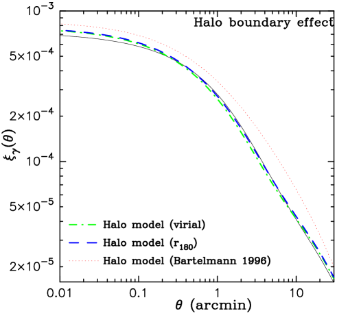
Figure 21: The figure shows how the halo boundary condition employed in the halo model calculation affects the prediction for $\xi_{\gamma}$. The thick dot-dashed and dashed curves are the results when we employ the NFW profile truncated at the virial radius and at the radius $r_{180}$, respectively. The radius $r_{180}$ is defined so that mean density enclosed by a sphere with radius $r_{180}$ is $180$ times the background density. The upper dotted curve shows the halo model prediction if one uses the expression in Bartelmann (1996) for the shear profile to compute the 1-halo term. For reference, the thin solid curve shows the Smith02 result in Figure 18.

Figure 21 explores how a modification of the halo boundary condition used in the halo model calculation affects the model prediction. As stated below equation (6), the Sheth-Tormen mass function (6) tends to better fit the mass function measured from $N$-body simulations, if one employs the halo mass estimator, $M_{180}$, enclosed within a region of the overdensity $\Delta_{180}(=180)$, than the virial mass estimator (e.g., White 2002). Therefore, one possible modification of the halo model is to employ the halo profile truncated at the radius $r_{180}$ . If we assume that the mass distribution in a halo follows an NFW profile up to $r_{180}$, we can obtain the relation between $M$ and $M_{180}$, which allows us to re-express all the relevant quantities in terms of the new mass $M_{180}$, as demonstrated in Hu & Kravtsov (2003). In addition, for consistency with the simulation results in White (2002), we employ the parameters of $a=0.67$ and $p=0.3$ for the Sheth-Tormen mass function (6) in the halo model calculation (see Table 2 in White 2002). The thick dashed curve plots the halo model prediction for $\xi_{\gamma}$ for the halo boundary $r_{180}$, while the thick dot-dashed curve is the result for the virial boundary. As can be seen, the two results are close, although the halo model of $r_{180}$ better matches the Smith02 result denoted by the thin solid curve over a range of the scale $0.\!\!^{\prime}5\lower 2.15277pt\hbox{$\;\buildrel<\over{\sim}\;$}\theta\lower 2.15277pt\hbox{$\;\buildrel<\over{\sim}\;$}5^{\prime}$. This is mainly due to the enhancement of the 1-halo term in the halo model with $r_{180}$, since $r_{180}>r_{\rm vir}$ ($\Delta_{v}=334>180$) for the $\Lambda$CDM model, hence the 1-halo term covers a larger range than the virial region. The dotted curve shows the halo model result when one employs the expression for the shear profile $\gamma_{M}$ in Bartelmann (1996) to compute the 1-halo term. The expression is derived by the line-of-sight projection of the NFW profile, allowing it to extend to infinite radius. It substantially overestimates the amplitude for $\xi_{\gamma}$ over the scales we have considered. Hence, if one intends to account for the mass contribution outside the virial region, it is necessary to first modify the mass defined within the new halo boundary and then to modify the halo model ingredients in terms of the new halo mass. This could improve the halo model accuracy over the transition scales between the non-linear and linear regimes, since the mass distribution outside the virial region is relevant for the quasi-linear regime ($\delta\sim 1$; also see the discussions around Figure 8 in TJ03b). We have confirmed that the boundary condition $r_{180}$ slightly improves the agreement between the halo model prediction for the lensing 3PCFs and the simulation results. However, in this paper, we implement the virial boundary for simplicity.

To summarize the results shown in Figures 18-19, we have shown that our real-space halo model formulation for cosmic shear statistics is self-consistent with the Fourier-space halo model. A great advantage of the real-space halo model is that it enables us to analytically compute any $n$-point correlation functions for both the convergence and shear fields on small angular scales, without additional computational effort compared to the two-point function.

Appendix B Convergence field for a generalized NFW profile

In this appendix, we present the convergence field around a generalized NFW profile with $\alpha\neq 1$ given in equation (10).

For general $\alpha$ the convergence field cannot be analytically computed. However, if $\alpha=0$ and $1$, we obtain analytical expressions to evaluate $\kappa_{M}$ in equation (13) in terms of $\Sigma_{M}$, which is given by

$$\Sigma_{M}(\theta)=\frac{Mc^{2}f_{0}}{2\pi r_{\rm vir}^{2}}F(c\theta/\theta_{\rm vir}),$$ (58)

with

$$F(x)=\left\{\begin{array}[]{ll}\displaystyle\frac{\sqrt{c^{2}-x^{2}}(2+c+x^{2}+2cx^{2})}{2(1+c)^{2}(1-x^{2})^{2}}-\frac{3}{2}\frac{x^{2}}{(1-x^{2})^{5/2}}{\rm arccosh}\frac{x^{2}+c}{x(1+c)},&(x<1)\\ \displaystyle\frac{\sqrt{c^{2}-1}}{5(1+c)^{3}}\left\{1+c(c+3)\right\},&(x=1)\\ \displaystyle\frac{\sqrt{c^{2}-x^{2}}(2+c+x^{2}+2cx^{2})}{2(1+c)^{2}(1-x^{2})^{2}}-\frac{3}{2}\frac{x^{2}}{(x^{2}-1)^{5/2}}{\rm arccos}\frac{x^{2}+c}{x(1+c)},&(1<x\leq c),\end{array}\right.$$ (62)

for $\alpha=0$ and

$$\Sigma_{M}(\theta)=\frac{Mc^{2}f_{2}}{2\pi r_{\rm vir}^{2}}F(c\theta/\theta_{\rm vir}),$$ (63)

with

$$F(x)=\left\{\begin{array}[]{ll}\displaystyle\frac{1}{x}{\rm arctan}\frac{\sqrt{c^{2}-x^{2}}}{x}-\frac{1}{\sqrt{1-x^{2}}}{\rm arccosh}\frac{x^{2}+c}{x(1+c)},&(x<1)\\ \displaystyle-\sqrt{\frac{c-1}{c+1}}+{\rm arctan}\sqrt{c^{2}-1},&(x=1)\\ \displaystyle\frac{1}{x}{\rm arctan}\frac{\sqrt{c^{2}-x^{2}}}{x}-\frac{1}{\sqrt{x^{2}-1}}{\rm arccos}\frac{x^{2}+c}{x(1+c)},&(1<x\leq c),\end{array}\right.$$ (67)

for $\alpha=2$, respectively. The factors $f_{0}$ and $f_{2}$ in the above equations are $f_{0}^{-1}=-c(2+3c)/(2(1+c)^{2})+\ln(1+c)$ and $f_{2}^{-1}=\ln(1+c)$. We again note that the convergence fields above are defined from the generalized NFW profile truncated at the virial radius, leading to $\Sigma_{M}(\theta)=0$ for $\theta>\theta_{\rm vir}$. These expressions are used to address the sensitivity of the lensing statistics to the inner slope parameter $\alpha$. Similarly, we can derive analytical expressions for the shear profiles for $\alpha=0$ and $2$, as in equation (16).

References

- [Bacon et al. 2002] Bacon, D., Massey, R., Refregier, A., Ellis, R., 2002, astro-ph/0203134
- [Bardeen et al. 1986] Bardeen, J. M., Bond, J. R., Kaiser, N., Szalay, A. S., 1986, ApJ, 304, 15
- [Barriga & Gaztañaga 2002] Barriga, J., Gaztañaga, E., 2002, MNRAS, 333, 443
- [Bartelmann 1996] Bartelmann, M., 1996, A&A, 313, 697
- [Bartelmann & Schneider 2001] Bartelmann, M., Schneider, P., 2001, Phys. Rep. 340, 291
- [Benitez & Martinez-Gonzalez 1997] Benitez, N., Martinez-Gonzalez, E., 1997, ApJ, 477, L27
- [Bernardeau et al. 2002a] Bernardeau, F., Mellier, Y., Van Waerbeke, L., 2002a, A&A, 389, L28
- [Bernardeau et al. 1997] Bernardeau, F., Van Waerbeke, L., Mellier, Y., 1997, A&A, 322, 1
- [Bernardeau et al. 2003] Bernardeau, F., Van Waerbeke, L., Mellier, Y., 2003, A&A, 397, 405, astro-ph/0201029
- [Bernardeau et al. 2002b] Bernardeau, F., Colombi, S., Gaztañaga, E., Scoccimarro, R., 2002b, Phys. Rep., 367, 1
- [Blandford et al. 1991] Blandford, R. D., Saust, A. B., Brainerd, T. G., Villumsen, J. V., 1991, MNRAS, 251, 600
- [Bond & Efstathiou 1984] Bond, J. R., Efstathiou, G., 1984, ApJ, 285, L45
- [Brown et al. 2002] Brown, M. L., Taylor, A. N., Bacon, D. J., Gray, M. E., Dye, S., Meisenheimer, K., Wolf, C., 2002, MNRAS, 341, 100
- [Bullock, Wechsler & Somerville 2002] Bullock, J. S., Wechsler, R. H., Somerville, R. S., 2002, MNRAS, 329, 246
- [Bullock et al. 2001] Bullock, J. S., Kolatt, T. S., Sigad, Y., Somerville, R. S., Kravtsov, A. V., Klypin, A. A., Primack, J. R., Dekel, A., 2001, MNRAS, 321, 559
- [Cooray & Hu 2001a] Cooray, A., Hu, W., 2001a, ApJ, 548, 7
- [Cooray & Hu 2001b] Cooray, A., Hu, W., 2001b, ApJ, 554, 56
- [Cooray & Sheth 2002] Cooray, A., Sheth, R., 2002, Phys. Rep., 372, 1
- [Crittenden et al. 2002] Crittenden, R. G., Natarajan, P., Pen, U.-L., Theuns, T., 2002, ApJ, 568, 20
- [Dahle et al. 2003] Dahle, H., Hannestad, S., Sommer-Larsen, J., 2003, ApJ, 588, L73
- [Dalal] Dalal, N., Kochanek, C. S., 2002, ApJ, 572, 25
- [Eisenstein & Hu 1999] Eisenstein, D. J., Hu, W., 1999, ApJ, 511, 5
- [Fukushige & Makino 1997] Fukushige, T., Makino, J., 1997, ApJ, 477, L9
- [Gaztañaga 2002] Gaztañaga, E., 2003, ApJ, 589, 82
- [Ghigna et al. 2000] Ghigna, S., Moore, B., Governato, F., Lake, G., Quinn, T., Steidel, J., 2000, ApJ, 544, 616
- [Guzik & Seljak 2002] Guzik, J., Seljak, U., 2002, MNRAS, 335, 311
- [Hamana & Mellier 2001] Hamana, T., Mellier, Y., 2001, MNRAS, 327, 169
- [Hamana et al. 2002] Hamana, T., et al., 2002, astro-ph/0210450
- [Hamana et al. 2003] Hamana, T., Kayo, I., Yoshida, N., Suto, Y., Jing, Y. P., 2003, astro-ph/0305187
- [Hamilton et al. 1991] Hamiltion, A. J. S., Matthews, A., Kumar, P., Lu, E., 1991, ApJ, 374, L1
- [Henry 2000] Henry, J. P., 2000, ApJ, 534, 565
- [Hoekstra et al. 2002] Hoekstra, H., Yee, H. K. C., Gladders, M. D., 2002, ApJ, 577, 595
- [Hu & Kravtsov 2003] Hu, W., & Kravtsov, A., 2003, ApJ, 584, 702
- [Hu & White 1997] Hu, W., & White, M. 1997, Phys. Rev. D., 56, 596
- [Hui 1999] Hui, L., 1999, ApJ, 519, L9
- [Jain 1997] Jain, B., 1997, MNRAS, 287,.687
- [Jain 2002] Jain, B., 2002, ApJ, 580, L3
- [Jain & Seljak 1997] Jain, B., Seljak, U., 1997, ApJ, ApJ, 484, 560
- [Jain, Mo & White 1995] Jain, B., Mo, H. J., White, S. D. M., 1995, MNRAS, 276, L25
- [Jain, Seljak & White 2000] Jain, B., Seljak, U., White, S. D. M., 2000, ApJ, 530, 547
- [Jarvis et al. 2003] Jarvis, M., Bernstein, G., Jain, B., Fischer, P., Smith, D., Tyson, J. A., Wittman, D., 2003, AJ, 125, 1014
- [Jenkins et al. 2001] Jenkins, A., Frenk, C. S., White, S. D. M., Colberg, J. M., Cole, S., Evrard, A. E., Couchman, H. M., P., Yoshida, N., 2001, MNRAS, 321, 372
- [Jing 1998] Jing, Y. P., 1998, ApJ, 503, L9
- [Jing & Suto 2000] Jing, Y. P., Suto, Y., 2000, ApJ, 529, L69
- [Jing & Suto 2002] Jing, Y. P., Suto, Y., 2002, ApJ, 574, 538
- [Kaiser 1992] Kaiser, N., 1992, ApJ, 388, 272
- [Kaiser 1998] Kaiser, N., 1998, ApJ, 498, 26
- [Kamionkowski et al. 1997] Kamionkowski, M., Kosowsky, A., & Stebbins, A., 1997, Phys. Rev. D., 55, 7368
- [Kamionkowski et al. 1998] Kamionkowski, M., Babul, A., Cress, C. M., & Refregier, A. 1998, MNRAS, 301, 1064
- [Limber 1954] Limber, D., 1954, ApJ, 119, 655
- [Ma & Fry 2000a] Ma, C.-P. Fry, J. N., 2000a, ApJ, 531, L87
- [Ma & Fry 2000b] Ma, C.-P. Fry, J. N., 2000b, ApJ, 538, L107
- [Ma & Fry 2000c] Ma, C.-P. Fry, J. N., 2000c, ApJ, 543, 503
- [McKay et al. 2001] McKay, T. A., et al., 2001, astro-ph/0108013
- [McClelland & Silk 1977] McClelland, J., Silk, J., 1977, ApJ, 217, 331
- [Ménard et al. 2003] Ménard, B., Hamana, T., Bartelmann, M., Yoshida, N., 2003, A&A, 403, 817
- [Mellier 1999] Mellier, Y., 1999, ARAA, 37, 127
- [Miralda-Escude 1991] Miralda-Escude, J., 1991, ApJ, 380, 1
- [Miyazaki et al. 2002] Miyazaki, S. et al. 2002, ApJ, 580, L97
- [Mo & White 1996] Mo, H. J., White, S. D. M., 1996, MNRAS, 282, 347
- [Mo, Jing & White 1997] Mo, H. J., Jing, Y. P., White, S. D. M., 1997, MNRAS, 290, 651
- [Moore et al. 1998] Moore, B., Governato, F., Quinn, T., Stadel, J., Lake G., 1998, ApJ, 499, L5
- [Nakamura & Suto 1997] Nakamura, T. T., Suto, Y., 1997, Prog. Theor. Phys., 97, 49
- [Navarro, Frenk & White 1996] Navarro, J., Frenk, C., White, S. D. M., 1996, ApJ, 462, 563
- [Navarro, Frenk & White 1997] Navarro, J., Frenk, C., White, S. D. M., 1997, ApJ, 490, 493 (NFW)
- [Neyman & Scott 1952] Neyman, J., Scott, E. L., 1952, ApJ, 116, 144
- [Padmanabhan, Seljak & Pen 2002] Padmanabhan, N., Seljak, U., Pen., U.-L., 2003, New Astron., 8, 581
- [Peacock & Doods 1996] Peacock, J. A., Dodds, S. J., 1996, MNRAS, 280, L19 (PD)
- [Peacock & Smith 2000] Peacock, J. A., Smith, R. E., 2000, MNRAS, 318, 1144
- [Peebles 1974] Peebles, P. J. E., 1974, A&A, 32, 197
- [Peebles 1980] Peebles, P. J. E., 1980, Large-Scale Structure of the Universe (Princeton: Princeton Univ. Press)
- [Pen et al. 2002] Pen, U., Van Waerbeke, L., & Mellier, Y., 2002, ApJ, 567, 31
- [Pen et al. 2003] Pen, U., Zhang, T., Van Waerbeke, L., Mellier, Y., Zhang, P., Dubinski, J., 2003, submitted to ApJ, astro-ph/0302031
- [Press & Schechter 1974] Press, W., Schechter, P., 1974, ApJ, 187, 425
- [Reblinsky & Bartelmann 1999] Reblinsky, K., Bartelmann, M., 1999, A&A, 345, 1
- [Refregier et al. 2002] Refregier, A., Rhodes, J., & Groth, E. J., 2002, ApJ, 572, L131
- [Scoccimarro & Frieman 1999] Scoccimarro, R., Frieman, J., 1999, ApJ, 520, 35
- [Scoccimarro & Sheth 2002] Scoccimarro, R., Sheth, R. K., 2002, MNRAS,329, 629 (PTHalos)
- [Scoccimarro et al. 2001] Scoccimarro, R., Sheth, R. K., Hui, L., Jain, B., 2001, ApJ, 546, 652
- [Scherrer & Bertschinger 1991] Scherrer, R. J., Bertschinger, E., 1991, ApJ, 381, 349
- [Schneider 2003] Schneider, P., 2003, astro-ph/0305240
- [Schneider & Lombardi 2003] Schneider, P., Lombardi, M., 2003, A&A , 397, 809 (SL03)
- [Schneider, Van Waerbeke & Mellier 2002a] Schneider, P., Van Waerbeke, L., Mellier, Y., 2002a, 389, 729
- [Schneider et al. 1998] Schneider, P., Van Waerbeke, L., Jain, B., Kruse, G., 1998, MNRAS, 296, 873
- [Schneider et al. 2002b] Schneider, P., Van Waerbeke, L., Kilbinger, M., Mellier, Y., 2002b, A&A, 396, 1, astro-ph/0206182
- [Seljak 2000] Seljak, U., 2000, MNRAS, 318, 203
- [Seljak & Zaldarriaga 1996] Seljak, U., Zaldarriaga, M., 1996, ApJ, 469, 437
- [Sheth & Jain 1997] Sheth, R., Jain, B., 1997, MNRAS, 285, 231
- [Sheth & Jain 2002] Sheth, R., Jain, B., 2002, submitted to MNRAS, astro-ph/0208353
- [Sheth & Lemson 1999] Sheth, R. K., Lemson, G., 1999, MNRAS, 304, 767
- [Sheth & Tormen 1999] Sheth, R. K., Tormen, G., 1999, MNRAS, 308, 119
- [Sheth et al. 2001] Sheth, R. K., Diaferio, A., Hui, L., Scoccimarro, R., 2001, MNRAS, 326, 463
- [Smith et al. 2002] Smith, R. E., Peacock, J. A., Jenkins, A., White, S. D. M., Frenk, C. S., Pearce, F. R., Thomas, P. A., Efstathiou, G., Couchman, H. M., P., 2002, astro-ph/0207664 (Smith02)
- [Somerville et al. 2001] Somerville, R. S., Lemson, G., Sigad, Y., Dekel, A., Kauffmann, G., White, S. D. M., 2001, MNRAS, 320, 289
- [Stebin 1996] Stebbins, A., 1996, astro-ph/9609149
- [Sugiyama 1995] Sugiyama, N., 1995, ApJS, 100, 281
- [Takada & Hamana 2003] Takada, M., Hamana, T., 2003, astro-ph/0305381
- [Takada & Jain 2002] Takada, M., Jain, B., 2002, MNRAS, 337, 875, astro-ph/0205055 (TJ02)
- [Takada & Jain 2003a] Takada, M., Jain, B., 2003a, ApJ, 583, L49, astro-ph/0210261 (TJ03a)
- [Takada & Jain 2003b] Takada, M., Jain, B., 2003b, MNRAS, 340, 580, astro-ph/0209167 (TJ03b)
- [Van Waerbeke 2000] Van Waerbeke, L., 2000, MNRAS, 313, 524
- [Van Waerbeke et al. 2001a] Van Waerbeke, L., Hamana, T., Scoccimarro, R., Colombi, S., Bernardeau, F., 2001a, MNRAS, 322, 918
- [Van Waerbeke et al. 2001b] Van Waerbeke, L., et al., 2001b, A&A, 374, 757
- [White 2002] White, M., 2002, ApJ Suppl., 143, 241
- [White, Van Waerbeke & Mackey 2002] White, M., Van Waerbeke, L., Mackey, J., 2002, ApJ, 575, 640
- [Wittman 2002] Wittman, D., 2002, astro-ph/0208063
- [Wright & Brainerd 2000] Wright, C. O., Brainerd, T. G., 2000, ApJ, 534, 34
- [Yano & Gouda 1999] Yano, T., Gouda, N., 1999, ApJ, 539, 493
- [Yoshida, Sheth & Diaferio 2001] Yoshida, N., Sheth, R., Diaferio, A., 2001, MNRAS, 328, 669
- [Zaldarriaga & Scoccimarro 2003] Zaldarriaga, M., Scoccimarro, R., 2003, ApJ , 584, 559 (ZS03)
- [Zaldarriaga & Seljak 1997] Zaldarriaga, M., & Seljak, U. 1997, Phys. Rev. D., 55, 1830
- [Zehavi et al. 2003] Zehavi, I., et al. 2003, submitted to ApJ, astro-ph/0301280