Carbon Monoxide Depletion in Orion B Molecular Cloud Cores
Abstract
We have observed several cloud cores in the Orion B (L1630) molecular cloud in the 2–1 transitions of C18O, C17O and 13C18O. We use these data to show that a model where the cores consist of very optically thick C18O clumps cannot explain their relative intensities. There is strong evidence that the C18O is not very optically thick. The CO emission is compared to previous observations of dust continuum emission to deduce apparent molecular abundances. The abundance values depend somewhat on the temperature but relative to ‘normal abundance’ values, the CO appears to be depleted by about a factor of 10 at the core positions. CO condensation on dust grains provides a natural explanation for the apparent depletion both through gas-phase depletion of CO, and through a possible increase in dust emissivity in the cores. The high brightness of HCO+ relative to CO is then naturally accounted for by time-dependent interstellar chemistry starting from ‘evolved’ initial conditions. Theoretical work has shown that condensation of H2O, which destroys HCO+, would allow the HCO+ abundance to increase while that of CO is falling.
keywords:
ISM: clouds – ISM: molecules – ISM: abundances – ISM: individual:Orion B – radio lines: ISM – radio continuum: ISM1 Introduction
There is considerable evidence that protostellar collapse occurs from an interstellar envelope (scale 104AU) onto, most likely, a circumstellar disc (scale 100 AU) . For a long time the collapse is likely to be isothermal and at a low temperature (about 10 K). This temperature is lower than the freeze-out temperatures of common interstellar molecules (CO 15–17 K, NH3 50–60 K, H2O 90 K; see Nakagawa 1980), and, as collapse proceeds, the freeze-out timescale becomes shorter than the collapse timescale. The expectation is for a long isothermal phase at 10 K when the molecules freeze-out onto grains followed by re-heating when they come off again. These processes have been modelled by, inter alia, Nejad, Williams & Charnley (1990), Rawlings et al. (1992), Bergin & Langer (1997) and Charnley (1997).
There is observational evidence for depletion in cores (by about an order of magnitude) in molecules such as CO and CS (e.g. Bergin et al. 2001; Tafalla et al. 2002). Most of these results have come from observations of nearby molecular cloud cores in which low-mass stars are forming in small groups (e.g. Jorgensen, Schöier & van Dishoeck 2002). In the more distant Orion region where our targets lie, NGC2024 (in L1630) contains several compact cores which show evidence for depletion of CO and other molecules (Mauersberger et al. 1992).
The interpretation as depletion has been criticised, however, by Chandler and Carlstrom (1996), who have provided evidence that some of the molecular gas is hot. Their criticisms include: (a) the dust opacity law in the cores will be non-standard, (b) dust emission may become optically thick at the short submm wavelengths – giving an ‘artificially low’ flux which is interpreted as a low temperature in an ‘optically thin’ interpretation, and (c) the cores may contain unresolved components which are highly optically thick in molecular lines - but thin in submillimetre dust emission. Thus the true molecular abundance may be much higher. Mangum et al. (1999) also provide evidence that the gas in the cores of NGC2024 is hot (40 K) which would accommodate a normal abundance for CO.
One problem with NGC2024, however, is that it is near strong external heat sources and HII emission and it is not clear that the line emission from the molecular gas arises from within the cores from which the dust emission emanates.
In this paper we report new observations of carbon monoxide isotopomers C18O, C17O and 13C18O from selected positions near and around cold cores in the same molecular cloud, L1630. These positions have been chosen with reference to previously published maps of HCO+, C18O and dust continuum emission from the condensations LBS23 (also known as HH24–26), LBS17, and LBS18 (e.g. Gibb et al. 1995; Gibb & Little 1998, 2000; Phillips, Gibb & Little 2001. These references will be quoted as GLHL, GL98, GL00, and PGL respectively). GL98 and GL00 deduced that there was depletion in several cores. The aim of this work is to confirm its significance and to evaluate its extent. We seek to determine optical depths from the CO isotopomers and use the previously published dust emission data together with a range of possible emission laws to examine the relative abundance.
In Sections 2 and 3 we justify our need to observe isotopomers as rare as 13C18O. In Section 4 we describe the observations, which we analyse in Section 5 to deduce the depletion in and around the cores. The chemical significance of the results is outlined in Section 6.
2 Proving depletion?
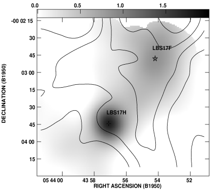
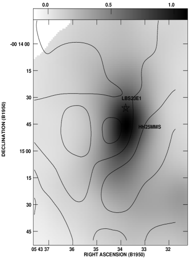
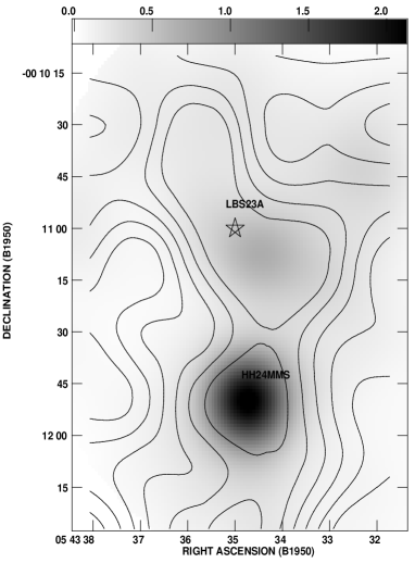
Maps of two of the largest cores in the Orion B molecular cloud, LBS17 and LBS23, made in high excitation HCO+ and C18O (J=21) lines , show striking differences between the structures traced by the two molecules. Particularly apparent is the enhanced brightness of =32 HCO+ relative to =21 C18O in the protostellar core LBS17-H (Fig. 2 of GL00), and of =43 HCO+ to =21 C18O in HH25MMS (Fig. 1 of GL98). Figs. 1, 2 and 3 show the relation between the C18O and dust emission. C18O emission is surprisingly weak in some of the clumps which stand out prominently in the other species. An interpretation assuming a simple source structure, optically thin C18O, and the dust emissivity law proposed by Hildebrand (1983), implies widespread reductions of the C18O abundance in these clumps by factors of 13 to 57 compared to what we take to be its canonical value of 210-7 (GL98 and Frerking, Langer & Wilson 1982). Most of the clumps appear to be bound objects of several solar masses (for LBS23 at least).
GL98 consider other ideas to explain the apparent reduction in abundance for the clumps in LBS23. Abnormal dust properties do not appear to be required because dust-emission-derived masses for the clumps are in good agreement with their virial masses.
Another possibility is the absorption of C18O emission from intervening low excitation temperature gas. If this were the case then the effect would be seen as strong self-absorption in the optically thicker CO lines. However, there is no evidence for such self-absorption in the CO spectra (GH93). Since the observed antenna temperatures measure the excitation temperature where the optical depth becomes equal to unity, a comparison of the CO and C18O antenna temperatures would then suggest that the cloud cores are externally heated (see e.g. GL98).
If the C18O emission arises in optically thick, unresolved sub-clumps the need for depletion might be avoided as all the C18O might not be detected. Accordingly we have made careful observations of weak isotopomers, including C18O, C17O and 13C18O, to seek to eliminate a sub-clump model. To illustrate how this can be achieved we consider a simple two-component model in the next section.
3 Optically thick clumping model
| Sub-clump model | Depletion | |||||
|---|---|---|---|---|---|---|
| Molecule | Sub-clump | (K) | (K) | Total | model | Observed |
| optical depth | sub-clump | Envelope | (K) | (K) | (K) | |
| C18O | 120 | 0.34 | 1.1 | 1.4 | 1.4 | 1.3 |
| C17O | 22 | 0.34 | 0.2 | 0.55 | 0.25 | 0.28 |
| 13C18O | 2 | 0.34 | 0.02 | 0.35 | 0.025 | 0.08 |
In Section 5 of GL98 the authors describe a two-component model (‘envelope’ and ‘sub-clump’) where the envelope (component 1) is optically thin (depth , linewidth ) in the less abundant CO isotopomers, such as C18O, and the sub-clump material (component 2) is optically thick (depth , linewidth ) in these same lines. Extending their analysis it is also possible to define an apparent depletion factor which describes how the presence of the optically thick clump mimics depletion within the beam in the simplistic interpretation as a single component. The CO abundance for such a source would be proportional to + . However, in the standard optically thin analysis, not knowing , we would assume the CO abundance is proportional to + . We will thus deduce CO abundances that are too low by a ratio
| (1) |
where is defined in GL98 as the ratio of the integrated intensities of components 1 and 2. The optical depth of the sub-clump component in the denominator causes to be less than unity, and demonstrates how an optically thick sub-clump can mimic depletion. If we assume that the abundance is in fact normal then we can use our model along with estimates of and to deduce information concerning the nature of the sub-clumps.
For example, the clump HH25MMS (GLHL, GL98 and PGL) stands out very prominently in dust continuum and 43 HCO+ emission but it is barely detectable as an independent source on the north-south ridge of 21 C18O emission. The integrated intensity on the ridge is typically 2.5 K km s-1 while HH25MMS adds about 0.8 K km s-1 to it. Thus . Also the apparent depletion factor, , is about 1/30 (according to GL98). Hence, from equation 1, = 120.
GL98 showed that the beam filling factor of the sub-clumps was given by
| (2) |
The 43 HCO+ emission is closely correlated with the continuum dust emission, rather than the C18O, but has a linewidth similar to the C18O so . Also for HH25MMS 0.2 so that the sub-clump filling factor is = 0.06. These would be sub-clumps with a very high C18O optical depth and a very small beam filling factor in the 22 arcsec JCMT beam.
We shall assume that the JCMT beam, of radius R, contains n identical sub-clumps of radius r. Then . We know since HH25MMS is resolved. It follows that arcsec or 1000 AU at the distance of L1630 (400 pc). Since the apparent depletion is high, most of the mass within the beam at HH25MMS is in the sub-clumps. GLHL quote a mass of 8 M⊙ in the core of HH25MMS. The sub-clump mass is then M⊙ and its density is greater than 2.5108 cm-3. The density of the envelope material is much lower. Its mass is 1/30th that of the clumps, and taking the mass to be within a beamwidth gives a density 5104 cm-3. In summary, if we seek to retain normal abundances by assuming sub-clumping it would appear that the sub-clumps must have radii less than 1000 AU and densities greater than 2.5108 cm-3.
As described by GL98, the most obvious problem with the ‘sub-clump’ interpretation seems to lie in the fact that the HCO+ intensity follows the submillimetre dust continuum emission well (rather than the envelope observable in C18O) yet its brightness temperature is so high that it must have a beam filling factor near unity, which is much greater than that deduced for the sub-clumps from C18O. Nonetheless it is important to test the structure within the clumps either via interferometric observations or beam-matched observations of weaker CO isotopomers.
We may predict C17O line intensities, assuming =120. The component 1 intensity should decrease by a factor of 5.4 compared to C18O, since it is optically thin, but that from component 2 will be unaltered as its optical depth will still be extremely high (=120/5.4). Referring to Table LABEL:clumps, the intensity will be
| (3) |
so the ratio of the C18O to C17O intensities will be 2.6. This might easily be misinterpreted as indicating that the C18O was just slightly optically thick. Observations of even rarer isotopomers – so that the optically thin ‘envelope’ contribution becomes negligible while the optically thick core component still remains – are required. Table LABEL:clumps gives predicted line intensities for the ‘depletion’ and ‘sub-clump’ models. It can be seen that observations of 13C18O are clearly capable of distinguishing between them.
4 Observations
4.1 CO observations
Observations of the J=21 transitions of C18O, C17O and 13C18O were carried out over the period of 1998 February 16–28 at the James Clerk Maxwell Telescope, using the common user SIS receiver A2 (Davies et al. 1992) and the digital autocorrelation spectrometer DAS. The original mixer in A2 had been replaced by one from NRAO. The C17O observations were made assuming a rest frequency of 224.714 GHz, the C18O observations at 219.560 GHz and the 13C18O observations 209.419 GHz. Key positions were selected from our previous maps of the cores, and, in addition, a new map of C18O in LBS18 was made. The positions chosen are listed in Table LABEL:pos. The positions of cores were observed, as well as a selection of references off core where there was sign of continuum emission.
The pointing and antenna temperature were measured with reference to the nearby source OMC1. The pointing was consistent typically to within about 3 arcsec. On 16th and 17th February the apparent antenna temperatures of lines from the frequently observed calibrating source OMC1 varied with time when observing the C18O and 13C18O lines. The intensity of the C18O line varied systematically with time between 0.51 and 0.80 of that of the Observatory reference spectrum for OMC1 C18O, = 7.5 K. The C18O intensities we quote have been systematically corrected for this variation, which brought three of the observations into agreement with similar ones described by GL98.
There was no appropriate Observatory reference for that part of the passband containing 13C18O or C17O. Although 13C18O was not clearly discernible for OMC1 on 16th February the intensities of several bright lines in the passband containing it varied systematically with time between 0.42 and 0.64 of their value on 18th and 19th February. It has been assumed that the values for 18th and 19th February are correct, and our 13C18O intensities scaled on this assumption. The C17O line observed in OMC1 showed no significant variation between 17th, 18th and 20th February, yielding = 1.90.1 K. This value has been assumed correct, and no scaling applied to our observed C17O intensities.
| Source | RA | DEC | Core? | ||||
|---|---|---|---|---|---|---|---|
| h | m | s | ∘ | ′ | ″ | ||
| HH24MMS | 05 | 43 | 34.7 | –00 | 11 | 49.0 | yes |
| HH25MMS | 05 | 43 | 33.8 | –00 | 14 | 45.0 | yes |
| LBS17H | 05 | 43 | 57.1 | –00 | 03 | 44.3 | yes |
| LBS18S | 05 | 43 | 54.2 | +00 | 18 | 23.0 | yes |
| LBS23E1 | 05 | 43 | 33.8 | –00 | 14 | 36.0 | no |
| LBS17F | 05 | 43 | 54.2 | –00 | 02 | 48.0 | no |
| LBS18A | 05 | 43 | 55.2 | +00 | 18 | 57.0 | no |
| LBS18B | 05 | 43 | 54.7 | +00 | 18 | 48.0 | no |
| LBS23A | 05 | 43 | 35.0 | –00 | 11 | 00.0 | no |
An observation of CO in OMC1 on 17th February yielded a line of brightness 0.9 of the observatory reference value. The reason for the time variation of C18O and 13C18O line intensities on 16th and 17th February has not been established. Based on the authors’ experience, possibilities might include incorrect adjustment of one of the telescope mirrors, problems in SIS receiver calibration (see, e.g. Davies et al. 1992) or uncertainty in receiver sideband calibration, though the latter might not be expected to vary with time. The receiver was tuned for double sideband performance and it is expected that the sideband ratio should be no worse than 1.2. Changing the LO frequency to observe the same C18O line in both sidebands on the 17th, when the observed strength was low (though not a measurement of the sideband ratio) produced very similar line intensities, tending to suggest that the sideband ratio was not responsible.
4.2 Continuum observations
The continuum observations used in this paper were made using the submillimetre bolometer array receiver SCUBA and are described in PGL. For the purposes of this paper we have smoothed their 850m maps to the same resolution as that of our CO data, i.e. 22 arcsec.
5 Results And Analysis
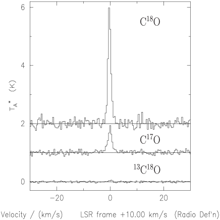
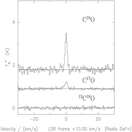
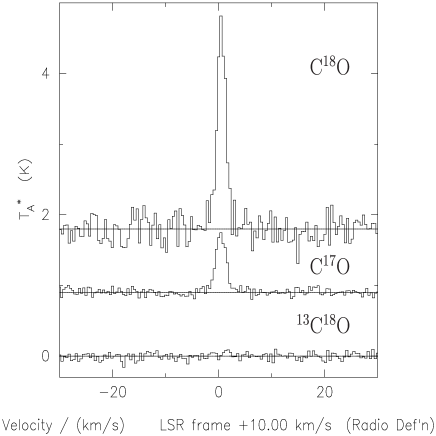
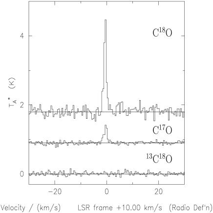
Table LABEL:intens contains the data taken from the new observations. The antenna temperatures, , derived from the CO observations for all three species at each of the positions are shown. The observations were made with a channel spacing and noise bandwidth of 0.45 kms-1. Four channels were averaged to give the temperatures quoted in Table LABEL:intens. (Note that the spectra are show in the original spectral resolution of 0.45 km s-1.) The integrated intensity (K km s-1), which is derived from the antenna temperature (=, integrated over 1.79 kms-1), for each species is also shown.
The Astronomical Image Processing Software (aips) package was used to analyse the continuum data. The 850 m and 450 m continuum emission maps were convolved to an effective resolution of 22 arcsec. The fluxes (Jy) for each position listed in Table LABEL:pos were then taken from the convolved maps and are listed in Table LABEL:intens. The uncertainty in these values is 0.02–0.03 Jy.
| C18O | C17O | 13C18O | 850 | ||||
|---|---|---|---|---|---|---|---|
| Source | |||||||
| (K) | (K km s-1) | (K) | (K km s-1) | (K) | (K km s-1) | (Jy) | |
| HH24MMS | 2.80.03 | 5.80.07 | 0.670.01 | 1.750.03 | 0.0570.020 | 0.090.03 | 4.76 |
| HH25MMS | 1.30.03 | 2.50.09 | 0.280.01 | 0.800.02 | 0.0800.045 | 0.020.05 | 2.36 |
| LBS17H | 2.60.03 | 6.00.07 | 0.640.01 | 1.800.03 | 0.0880.048 | 0.160.06 | 3.79 |
| LBS18S | 1.50.03 | 3.00.16 | 0.370.01 | 0.800.03 | 0.0720.048 | 0.020.06 | 1.34 |
| LBS23E1 | 1.80.06 | 3.40.15 | 0.300.02 | 0.800.05 | — | — | 1.97 |
| LBS17F | 3.90.06 | 7.30.15 | 0.900.02 | 2.200.05 | — | — | 1.85 |
| LBS18A | 2.60.06 | 3.00.15 | 0.450.02 | 0.750.05 | — | — | 0.82 |
| LBS18B | 3.00.06 | 3.40.13 | 0.420.02 | 0.900.05 | — | — | 0.85 |
| LBS23A | 2.60.10 | 6.00.23 | — | — | 0.050.015 | 0.120.02 | 1.08 |
5.1 Temperatures and masses
From the fluxes at 850 m and 450 m we seek to derive the temperatures and masses. The results depend on the opacity law, which is uncertain. Rather than seeking to justify a law we chose to investigate the effect of varying it by comparing the different results obtained assuming two typical but reasonably extreme examples: the laws proposed by Hildebrand (1983) (=2) and by Testi & Sargent (1998) (=1.1). These predict very similar opacities at 850 m, but different temperatures from 850/450 flux ratios. We accordingly derive temperatures from both these laws, and compare them with already published temperatures from grey body spectral fits and ammonia inversion line observations to deduce plausible temperature limits. These are then used with the 850 m opacities to deduce masses.
If the absorption coefficient is written in terms of the dust and molecular hydrogen density as
| (4) |
the total number of hydrogen molecules implied by observation of a flux , from dust assumed to be optically thin, is
| (5) |
where is the distance from Earth.
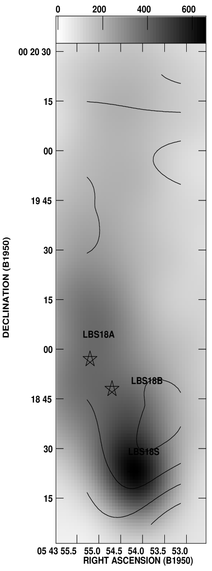
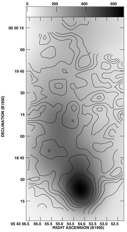
The temperature of the gas can be derived by forming the ratio of the submillimetre continuum fluxes at the two wavelengths and comparing it with that predicted for different temperatures using equation 5. Flux-ratio maps were produced by using the comb task in aips to divide the 850 m (15 arcsec resolution) maps by the 450 m (15 arcsec resolution) maps. The ratio, (850/450), was measured at each point from these maps and used to find the temperature. The flux-ratio map of LBS18, which has been smoothed to a resolution of 22 arcsec, has been plotted over the 850 m (22 arcsec) continuum map in Fig. 9, where it can be seen that the contours representing the higher values of (850/450) are coincident with the dust peaks. This may be due to (a) a lower temperature, (b) a flatter emissivity law, or (c) the 450 m emission being optically thick.
The resulting value of for each position can be found in Table LABEL:temps for both values of . As expected, the temperatures are higher for the lower value of . The errors are derived using the calibration uncertainties and random noise errors quoted in PGL.
Assuming the dust is optically thin can produce misleadingly low temperatures and high derived masses if the dust is in fact optically thick at 450 m. However PGL used a radiative transfer program to model the cores that was not limited by this assumption, but derived very similar temperatures to those found here. In reality the results we find represent an average over the beam. It is also quite likely that there are temperature gradients within the beam, either decreasing towards the centre of the core (e.g., an externally heated protostellar cloud) or increasing (e.g., an interstellar cloud heated by a central young star). If there are, then the derived beam–averaged temperature will be weighted towards the hotter dust which radiates more strongly. This means that the derived dust masses will be too low (colder dust being underweighted). CO column densities are less sensitive to temperature, so the overall effect is to derive CO abundances which are higher than the true ones – i.e. to make the depletion appear less marked than it really is.
| Source | ||||
|---|---|---|---|---|
| HH24MMS | 205 | 10 | 71 | 153 |
| HH25MMS | 17–35 | 38 | 13 | 152 |
| LBS17H | 20 | 14 | 9 | — |
| LBS18S | — | 14 | 9 | — |
| LBS23E1 | — | 37 | 13 | — |
| LBS17F | — | 16 | 9 | — |
| LBS18A | — | 23 | 11 | — |
| LBS18B | — | 24 | 11 | — |
| LBS23A | — | 37 | 13 | — |
Further information is available which can be used to constrain the temperatures. Grey body fits to the spectra of dust continuum emission give =17–35 K for HH25MMS (Gibb and Davis, 1998), =205 K for HH24MMS (Ward-Thompson et al., 1995) and 20 K for LBS17H (GL00). It is also of interest to compare the derived temperatures with those obtained from NH3 inversion lines. Harju et al. (1993) used NH3(1,1) and (2,2) observations of 40 arcsec resolution to derive the kinetic temperature of 43 star forming cores, 16 of which are associated with the Orion L1630 and L1641 clouds. They mapped LBS23, finding temperatures of about 15K at the positions of HH24MMS and HH25MMS. These results and those from the grey body fits are included in Table LABEL:temps. In general the kinetic temperature shows little variation over their maps. Their results show that the average kinetic temperature is 15.7 K for the Orion cores. Only two of their cores showed temperatures greater than 20 K. Matthews and Little (1983) also mapped LBS23 with 130 arcsec resolution; at HH25 they found a temperature of 14 K which is similar to that of Harju et al. As the cloud is extended and their beam contained a substantial region surrounding the core it is likely that a temperature of 14 K is representative of the envelope surrounding the core.
On the basis of Table LABEL:temps and the general considerations above we regard conservative limits for the dust temperatures to be 205 K for HH24MMS and HH25MMS and 155 K for LBS17H and LBS18S, while for the off–core envelope positions we take =155 K. We then use these temperatures and the 850 m fluxes together with the 850 m opacity of Testi and Sargent to deduce gas masses via equation 5. These are used in Section 5.3 to derive relative CO abundances.
5.2 Carbon monoxide optical depths
We can see immediately that the observed isotope line ratios listed in Table LABEL:clumps for HH25MMS are in much better agreement with the predictions of the depletion model than with those for optically thick sub-clumps. It should be noted that although optically thick undepleted sub-clumps are unlikely to explain the apparent depletion the existence of depleted clumps is not ruled out.
Table LABEL:tau shows the line temperatures and their ratios ((18/17), denoting the ratio of and , the line temperatures of C18O and C17O respectively). The mean value of (18/17) in the cores is 4.28; towards the other positions 6.1. The latter value is in good agreement with the solar expectation of 5.4, suggesting that these positions are optically thin, and that the [C17O]/[C18O] ratio is normal. The former suggests that C18O may be slightly optically thick in the cores, but certainly not sufficiently to discredit a former conclusion that CO is depleted in several of the cores of LBS23 (GL98). The [C17O]/[13C18O] ratios are consistent with the solar value.
The above constitutes good evidence that C17O and 13C18O are optically thin.
The optical depths of the three species in the individual positions have been calculated. Firstly, the optical depth of C17O can be calculated using equation 6, where is the line temperature of C17O and is that of C18O and and are the optical depths of C17O and C18O respectively.
| (6) |
By assuming that solar values hold, = 5.4, equation 6 was solved to obtain a value for at each position. The values of are displayed in Table LABEL:tau with the errors calculated for each value. Multiplying by 5.4 gives at each position. One can also calculate , the optical depth of 13C18O by dividing by 16.6. It can be seen from these results that all three species of CO are optically thin in the regions where the abundances have been calculated and can therefore be used effectively in the calculations. The negative optical depth values in Table LABEL:tau are likely to be due to noise errors, rather than weak maser emission.
| Source | (18/17) | ||||
|---|---|---|---|---|---|
| (K) | (K) | ||||
| HH24MMS | 0.67 | 2.8 | 4.2 | 0.12 | 0.02 |
| HH25MMS | 0.28 | 1.3 | 4.6 | 0.08 | 0.04 |
| LBS17H | 0.64 | 2.6 | 4.1 | 0.13 | 0.02 |
| LBS18S | 0.37 | 1.5 | 4.1 | 0.13 | 0.04 |
| LBS23E1 | 0.30 | 1.8 | 6.0 | -0.05 | 0.02 |
| LBS17F | 0.90 | 3.9 | 4.3 | 0.11 | 0.03 |
| LBS18A | 0.45 | 2.6 | 5.8 | -0.03 | 0.05 |
| LBS18B | 0.42 | 3.0 | 7.1 | -0.12 | 0.05 |
| LBS23A | — | 2.6 | 7.3 | -0.13 | — |
5.3 Relative abundance of CO
For an optically thin transition the total number of molecules within a beam (FWHM arcsec) from a source at D (kpc) is given by
| (7) |
where is the rotational constant (GHz), the dipole moment (debyes), the upper level of the transition, is the fractional population of level , is the integrated line intensity (K km s-1), and is given by
| (8) |
where is the cosmic microwave background temperature (2.7 K).
The relative abundance of the CO isotopomer can be estimated by computing from equation LABEL:NMOL and dividing by from equation 5. (To calculate the relative abundance, the integrated intensities in Table LABEL:intens were divided by to correct for beam efficiency.)
The C18O abundance, , was calculated in the same way as for C17O and 13C18O but the answers obtained for HH24MMS, HH25MMS, LBS17H, LBS18S, and LBS17F, were multiplied by (5.4/), where =(18/17) (see Table LABEL:tau), to allow for the finite optical depth of C18O. The resulting relative abundances of C17O, C18O and 13C18O at each position can be found in Table LABEL:abund.
| Source | ||||
|---|---|---|---|---|
| (K) | ||||
| HH24MMS | 205 | 2.4 | 0.6 | 2.8 |
| HH25MMS | 205 | 1.9 | 0.5 | 1.3 |
| LBS17H | 155 | 2.0 | 0.5 | 4.1 |
| LBS18S | 155 | 2.9 | 0.6 | 1.5 |
| LBS23E1 | 155 | 1.7 | 0.4 | — |
| LBS17F | 155 | 4.8 | 1.2 | — |
| LBS18A | 155 | 3.6 | 0.9 | — |
| LBS18B | 155 | 3.9 | 1.0 | — |
| LBS23A | 155 | 5.4 | — | 10.8 |
6 Discussion
6.1 Morphology
It appears, from comparing SCUBA and line results, that the cores tend to be found on the edges or ends of filaments. There are two kinds of core structure: ones where the HCO+ and dust are coincident but C18O is very faint or absent (LBS17H, HH24MMS), others where HCO+, C18O and dust peak successively towards the cloud edge (LBS18S and the Launhardt et al. (1996) core in LBS17 (see GL00)). The problem is to distinguish the effects of chemistry and excitation.
6.2 Depletion
The canonical values for the abundance of C18O, C17O and 13C18O may be taken to be , and, assuming simple proportion, respectively, from Frerking et al. (1982). Dividing these values by the corresponding abundances in each position, one can estimate the depletion factor, , for each isotopomer. Table LABEL:depl displays these depletion factors and one can see that in all cases the CO is depleted significantly.
Relative to the canonical values, the isotopic species appear to be depleted by factors of about 10 on the cores, and approximately half that in the envelopes. The values are typically less than those quoted by GL98, the differences being due to the assumption of slightly higher temperatures, careful matching of effective beam sizes and correction for the optical depths of C18O.
A natural explanation for the depletion observed in these cores is the condensation of CO molecules on dust grains since the density (106 cm-3: GLHL, GL98) is high enough to reduce the freeze-out timescale to less than the dynamical timescale. In addition, grain growth by coagulation is expected in such regions which gives rise to increased dust emissivity (Ossenkopf 1993). The consequence of these two processes is that dense collapsing cores become very well defined in submillimetre continuum emission while simultaneously becoming very poorly defined in C18O emission, such as we observe here.
A number of studies of other star-forming regions have also arrived at the conclusion that the CO abundance is lower than the canonical value. Studies by Kramer et al. (1999), Willacy, Langer & Velusamy (1998) and Caselli et al. (1999) have found that the C18O abundance is reduced typically by factors ranging from a few to an order of magnitude towards the lines of sight with highest H2 column density. The study of Kramer et al. (1999) shows that the highest reduction in the C18O abundance occurs in the coldest regions. In all cases, these authors also conclude that freeze out of CO onto cold dust grains is responsible for the observed levels of depletion.
| Source | (K) | |||
|---|---|---|---|---|
| HH24MMS | 205 | 8.5 | 8.5 | 9.5 |
| HH25MMS | 205 | 10.7 | 9.2 | 21.3 |
| LBS17H | 155 | 9.8 | 10.2 | 6.6 |
| LBS18S | 155 | 7.0 | 8.1 | 18.6 |
| LBS23E1 | 155 | 11.9 | 11.8 | — |
| LBS17F | 155 | 4.1 | 4.0 | — |
| LBS18A | 155 | 5.6 | 5.3 | — |
| LBS18B | 155 | 5.1 | 4.6 | — |
| LBS23A | 155 | 3.7 | — | 2.5 |
Although this investigation has shown that CO appears to be depleted in the cores, one cannot be sure that the factors are correct, as we are calculating the abundance using averages along the line of sight. If, for example, the cores are much colder than the envelopes, there will be a higher depletion factor in the cores and a lower one in the envelopes. This is one area which needs to be studied further in order to find a way of deriving the emission produced at the core positions rather than averaged along the line of sight. One must also keep in mind that the canonical values of the abundance have been calculated using line of sight observations which may contain dust and gas that is a lot less dense than that found in protostellar cores so comparing the core abundances with these values may not give a true depletion factor.
6.3 Implications for chemical models
Rawlings et al. (1992) show that as a protostar collapses it is plausible that the chemistry occurring while molecules deplete out onto dust grains leads to an increasing HCO+/CO ratio (by up to 50), although their absolute abundances finally fall. A requirement for this to happen is a high initial H2O abundance such as might result from initial conditions following a shock through already processed material, but not from initial conditions which are of simple atomic form.
Observations of water have been made towards the regions encompassing HH24MMS and HH25MMS with ISO, but these only trace a hot dense component in shocked gas (Benedettini et al. 2000). Perhaps more reliable but still less than ideal are the observations of NGC2024 with the Submillimeter-Wave Astronomy Satellite (SWAS) by Snell et al. (2000). Snell et al. estimate that the abundance of water (strictly only the ortho species) to be , considerably lower than expected but in agreement with the notion of ongoing and widespread depletion by freeze out onto dust grains.
Other models have been developed which have different assumptions. Bergin & Langer (1997) followed chemistry during the collapse using a gas-grain chemical code, including desorption and depletion, but starting from an initial pristine state with elements only. The increase in HCO+/CO suggested by observations was not produced by the model. Neither was it produced by the different type of model of Charnley (1997).
Bergin et al. (2000) have proposed an alternative method of reducing the CO abundance, prompted by results from SWAS. In their model CO abundance can drop (even in warm clouds, say, 30 K) as a result of destruction by He+ with the oxygen atoms freezing out and becoming locked in water ice. Unfortunately their discussion excludes HCO+, and it should also be noted that the CO destruction occurs on extremely long timescales (greater than a million years), much longer than the collapse timescales for these cloud cores.
The model of Rawlings et al. (1992) predicts an abundance for HCO+ in good agreement with a value we have derived for HH25MMS (, GLHL). In addition, the modelling of Caselli et al. (2002) shows that the HCO+ abundance may be used to estimate the maximum degree of depletion. Their Model 3 (shown in their Fig. 8) also predicts a value for the HCO+ abundance close to our LVG estimate for HH25MMS. At this value (which is also at a radius close to the beam radius for our JCMT observations) the depletion factor is 20, in good agreement with the levels of CO depletion we derived above.
However,it should also be noted that from our LVG modelling (GLHL) we find that the HCO+ is optically thick, and thus any decrease in the HCO+ abundance in the centre of these cores (at radii less than 3000–4000 AU) is masked. Observations and modelling of rarer species will help to answer this question. We are currently analysing observations of HCO+ and DCO+ isotopomers on the cores to study this phenomenon more carefully.
Since star-formation has already taken place in L1630 (e.g. Lada et al. 1991) the initial conditions for the chemistry will not be pristine. This supports our consideration of the model of Rawlings et al. (1992), which starts from ‘evolved’ conditions (including a high abundance of water). Only this model predicts an actual increase of HCO+ while CO is declining. It thus provides a natural explanation for the brightness of high excitation HCO+ emission relative to CO emission on cores. It thus appears that the role of the initial conditions is very important in determining the later behaviour of the chemistry.
7 Conclusions
We have used new observations of C17O, C18O and 13C18O along with existing 450 m and 850 m continuum observations to study four regions in the Orion B molecular cloud. This has allowed the determination of optical depths for the isotopic species and the elimination of a model by which the cores contain many optically thick sub-clumps to explain the low isotopic CO emission.
If the dust emissivity falls within what are presently considered to be reasonable limits, CO is depleted in both the cores and the surrounding regions, but by a higher factor in the cores. Relative to the canonical abundances of Frerking et al. (1982), the CO appears to be depleted by about a factor of 10 at the core positions and a factor of 5 in the envelopes. Although the dust observations do not allow the temperatures to be constrained for =1.1, we believe it unlikely, from the NH3 observations of Harju et al. (1993) and Matthews and Little (1983), that temperatures will be greater than 15–20 K. It seems unlikely that the temperatures exceed the dust derived values in the sources.
The low abundance of CO and the brightness of HCO+ emission in the cores tends to support the model of Rawlings et al. (1992) which suggests that the amount of HCO+ in the core increases as that of CO decreases. The HCO+ abundance and observed levels of CO depletion are also in good agreement with a recent model of molecular ion chemistry in collapsing cores by Caselli et al. (2002).
Acknowledgments
The authors would like to thank the JCMT staff for their efforts in obtaining the observational data. The JCMT is operated by the Joint Astronomy Centre on behalf of the Particle Physics and Astronomy Research Council of the United Kingdom, The Netherlands Organization for Scientific Research and the National Research Council of Canada. We would also like to thank the referee for all the useful comments and suggestions. D Savva would like to thank PPARC for the award of a studentship.
References
- [1] Benedettini M., Giannini T., Nisin B., Tommasi E., Lorenzetti D., Di Giorgio A.M., Saraceno P., Smith H.A., et al., 2000, A&A, 359, 148
- [2] Bergin E.A., Ciardi R., Lada C.J., Alves J., Lada E.A., 2001, ApJ, 557, 209
- [3] Bergin E.A., Langer W.D., 1997, ApJ, 486, 316
- [4] Bergin E.A., Melnick G.J., Stauffer J.R., Ashby M.L.N., Chin G., Erickson N.R., Goldsmith P.F., Harwit M., et al., 2000, ApJ, 539, L129
- [5] Caselli P., Walmsley C.M., Tafalla M., Dore L., Myers P.C., 1999, ApJ, 523, L165
- [6] Caselli P., Walmsley C.M., Zucconi A., Tafalla M., Dore L., Myers P.C., 2002, ApJ, 565, 344
- [7] Chandler C.J., Carlstrom J.E., 1996, ApJ, 466, 338
- [8] Charnley S.B., 1997, MNRAS, 291, 455
- [9] Davies S.R., Cunningham C.T., Little L.T., Matheson D.N., 1992, Int.J.IR & MM Waves, 13, 647
- [10] Frerking M. A., Langer W. D., Wilson R. W., 1982, ApJ, 262, 590
- [11] Gibb A.G., Davis C.J., 1998, MNRAS, 298, 644
- [12] Gibb A.G., Heaton B.D., 1993, A&A, 276 511
- [13] Gibb A.G., Little L.T., Heaton B.D., Lehtinen, K.K., 1995, MNRAS, 277, 341 (GLHL)
- [14] Gibb A.G., Little L.T., 1998, MNRAS, 295, 299 (GL98)
- [15] Gibb A.G., Little L.T., 2000, MNRAS, 313, 663 (GL00)
- [16] Harju J., Walmsley C.M., Wouterloot J.G.A., 1993, A&AS, 98, 51
- [17] Hildebrand R.H., 1983, QJRAS, 24, 267
- [18] Jorgensen J.K., Schöier F.L., van Dishoeck E.F., 2002, A&A, in press.
- [19] Kramer C., Alves J., Lada C.J., Lada E.A., Sievers A., Ungerechts H., Walmsley C.M., 1999, A&A, 342, 257
- [20] Lada E.A., DePoy D.L., Evans N.J., Gatley I., 1991, ApJ 371, 171
- [21] Launhardt R., Mezger P.G., Haslam C.G.T., Kreysa E., Lemke R., Sievers A., Zylka R., 1996, A&A, 312, 569
- [22] Mangum J.G., Wootten A., Barsony M., 1999, ApJ, 526, 845
- [23] Matthews N., Little L.T., 1983, MNRAS, 205, 123
- [24] Mauersberger R., Wilson T.L., Mezger P.G., Gaume R., Johnston K.J., 1992, A&A, 256, 640
- [25] Nakagawa N., 1980, IAUS, 87, 365
- [26] Nejad L.A.M., Williams D.A., Charnley S.B., 1990, MNRAS, 246, 183
- [27] Ossenkopf V., 1993, A&A, 280, 617
- [28] Phillips R.R., Gibb A.G., Little L.T., 2001, MNRAS, 326, 927 (PGL)
- [29] Rawlings J.M.C., Hartquist T.W., Menten K.M., Williams D.A., 1992, MNRAS, 255, 471
- [30] Snell R.L., Howe J.E., Ashby M.L.N., Bergin E.A., Chin G., Erickson N.R., Goldsmith P.F., Harwit M., et al., 2000, ApJ, 539, L101
- [31] Tafalla M., Myers P.C., Caselli P., Walmsley C.M., Comito C., 2002, ApJ, 569, 815
- [32] Testi L., Sargent A.I., 1998, ApJ, 508L, 91
- [33] Ward–Thompson D., Chini R., Krugel E., Andre P., Bontemps S., 1995, MNRAS, 274, 1219
- [34] Willacy K., Langer W.D., Velusamy T., 1998, ApJ, 507L, 171