Decaying neutron propagation in the Galaxy and
the Cosmic Ray anisotropy at 1 EeV

Abstract

We study the cosmic ray arrival distribution expected from a source of neutrons in the galactic center at energies around 1 EeV and compare it with the anisotropy detected by AGASA and SUGAR. Besides the point-like signal in the source direction produced by the direct neutrons, an extended signal due to the protons produced in neutron decays is expected. This associated proton signal also leads to an excess in the direction of the spiral arm. For realistic models of the regular and random galactic magnetic fields, the resulting anisotropy as a function of the energy is obtained. We find that for the anisotropy to become sufficiently suppressed below $E\sim 10^{17.9}$eV, a significant random magnetic field component is required, while on the other hand, this also tends to increase the angular spread of the associated proton signal and to reduce the excess in the spiral arm direction. The source luminosity required in order that the right ascension anisotropy be $4\%$ for the AGASA angular exposure corresponds to a prediction for the point-like flux from direct neutrons compatible with the flux detected by SUGAR. We also analyse the distinguishing features predicted for a large statistics southern observatory.

1 Introduction

The distribution of the arrival directions of high energy Cosmic Rays (CRs) provides a useful tool to investigate their origin. This distribution is found to be very close to isotropic up to the highest energies measured. For energies below the knee ($E_{knee}\simeq 3\times 10^{15}$ eV) the measured anisotropy is below $0.1\%$, showing a smooth increase for larger energies and approaching the percent level around $10^{18}$ eV [1]. This isotropy is understood as due to the diffusive motion of charged particles in the galactic magnetic field for energies such that $E/Z\leq 10^{17}$ eV, with $Z$ the CR charge. Cosmic rays from galactic sources remain trapped in this field, leading to a flux building up at small energies and to the absence of correlations between the arrival direction of CRs and the source’s direction. At energies above $10^{19}$ eV, and up to the highest observed energies, the distribution of the events is compatible with isotropy. However, at these energies CRs are no more trapped in the galactic magnetic field, so that a correlation between the arrival and the source directions is to be expected. The absence of a significant correlation between ultra high energy events and the Galactic plane points then to extragalactic sources as the origin of these events.

In 1999 the AGASA group reported the measurement of the most significant anisotropy detected so far [2]. They presented the results of a search for anisotropies in the arrival directions of cosmic rays with energy above $10^{17}$ eV, using data collected over 11 years. They found a strong anisotropy of amplitude $\sim 4\%$ in a small energy range: $10^{17.9}-10^{18.3}$ eV. The phase of the first harmonic in right ascension was found to be $\alpha_{1}\simeq 300^{\circ}$. A two dimensional map showed that this anisotropy can be interpreted as due to excesses of events in two regions of size $\sim 20^{\circ}$ near the galactic center (GC) and the Cygnus region with significance $4\sigma$ and $3\sigma$, respectively. A subsequent analysis by the same group, including an independent data set, confirmed the initial claim [3].

Taking into account that the excess reported by AGASA lies close to the galactic center, that is better seen from the south, the SUGAR group reanalyzed their data [4]. The SUGAR experiment, located near Sidney, has a clear view of the GC, but has much poorer statistics than AGASA. They set a priori the energy range corresponding to the AGASA anisotropy and found a point like excess at $7.5^{\circ}$ from the GC, and $6^{\circ}$ away from the AGASA maximum. Due to the difference in direction and angular extension of the AGASA and SUGAR signals it is not yet clear whether they are consistent among each other and if they can result from a common origin.

A possible explanation of the anisotropy, already proposed by Hayashida et al. [2], is that it is due to neutron primary particles. Neutrons of $10^{18}$ eV have a Lorentz factor $\gamma\simeq 10^{9}$, so that their decay length is about 10 kpc, i.e. similar to the distance from the Earth to the galactic center. Hence, neutrons from a source near the galactic center can propagate up to the Earth before decaying, and they are undeflected by intervening magnetic fields, contrary to the case of charged primaries. The lack of significant anisotropies at smaller energies is explained within this scenario as due to the shorter decay length of the neutrons, and at larger energies by a cutoff in the acceleration energy (or due to a very steep spectrum) of the sources. They suggested that neutrons can be produced by accelerated heavy nuclei which disintegrated due to interactions with ambient matter or photons surrounding the source. Charged particles could stay confined by the magnetic fields present in the acceleration region, while neutrons would escape easily.

Medina-Tanco and Watson [6] proposed that a more likely way of generating a high energy neutron flux is through high energy protons via interactions with ambient protons or with infra red photons. They found that the neighborhood of the Galaxy’s central supermassive black hole could give the environment needed for these reactions to happen frequently enough. Nagataki and Takahashi showed that the proton-proton process was the most efficient one, and also studied the detectability of the $\gamma$ and $\nu$ emission associated to the production of neutrons in the GC [7].

The possibility that the GC is a source of high energy protons was studied by Levinson and Boldt [8]. They showed that, under certain conditions, a compact black hole dynamo associated with the Sgr A* source may accelerate protons up to energies $\sim 10^{18}$ eV, with a total luminosity of $\sim 10^{38}$ erg/s.

In this work, we study in detail the CR arrival direction distribution expected from a source of neutrons in the GC. The fact that the decay length of $10^{18}$ eV neutrons is similar to the distance to the proposed source implies that a sizable fraction of the neutrons will actually decay to protons before reaching the Earth, and the trajectories of these secondary protons will be bent by the galactic magnetic fields (GMF). These protons would arrive to the Earth from some preferred directions in the sky: those produced near the Earth would come from directions close to the GC one, while those produced in the inner Galaxy region would arrive preferentially from directions close to the spiral arm, as their trajectories wind around the regular magnetic field lines. Initial work in this direction was performed by Medina-Tanco and Watson [6] and here we extend it to take into account different allowed magnetic field strengths, we map the arrival direction distribution for different energies and take into account the angular exposure of experiments at different latitudes to study several features of the observations such as the energy dependence of the anisotropies, the compatibility of the observations of AGASA and SUGAR both regarding the angular extent of the observed features and the required source luminosity.

Other suggested explanations for the observed anisotropies include a diffusive flux of charged particles from the GC direction [9], the drift of heavy nuclei in the galactic magnetic field [10] and a source of protons in the galactic center [11, 12].

2 Cosmic Ray propagation in the Galaxy

The trajectories of charged CRs will be determined by the galactic magnetic field, which has both a large scale regular component and a random component, both with strengths of a few $\mu$G. The magnetic lines of the regular field follow the spiral structure, reversing direction between consecutive arms. According to the preferred model for our galaxy, it is symmetric with respect to the galactic plane. The strength of the field can be modeled as [15, 14]

$$B_{sp}(\rho,\theta,z)=B_{0}\frac{r_{0}}{2\rho}\tanh^{3}\left(\frac{\rho}{\rho_{1}}\right)\ \cos(\theta-\beta\ \ln\frac{\rho}{\xi_{0}})$$

$$\bigg{(}\frac{1}{\cosh(z/z_{1})}+\frac{1}{\cosh(z/z_{2})}\bigg{)},$$ (1)

where $(\rho,\theta,z)$ are cylindrical coordinates with origin in the galactic center, $\xi_{0}=10.55$ kpc is the value of $\rho$ for which the field is maximum in our spiral arm, $\beta=1/\tan\ p=-5.67$, where $p=-10^{\circ}$ is the pitch angle and $r_{0}=8.5$ kpc is the distance from the Sun to the GC. The overall intensity is taken as $B_{0}=3~{}\mu$G, corresponding to a local strength of the regular component close to $2~{}\mu$G. The $\tanh$ term smoothes the $1/\rho$ behavior of the field near the center within a core radius taken as $\rho_{1}=2$ kpc. The vertical scale length associated to the disk field is taken as $z_{1}=0.3$ kpc, while the halo one as $z_{2}=4$ kpc.

The radial and azimuthal components are given by $B_{\rho}=B_{sp}\ \sin~{}p$ and $B_{\theta}=B_{sp}\ \cos~{}p$ respectively, while the strength of the field in the $z$ direction is assumed to vanish.

Besides the regular magnetic field structure, a random component due to turbulence in the interstellar plasma is known to exist, with the largest eddies having a scale of $L_{max}\simeq 100$ pc. A usual assumption is that the spectrum of the field inhomogeneities is the same as that of the gas density, that is close to a Kolmogorov spectrum. Hence, the turbulent magnetic field can be described by a random field with a power law spectrum such that the magnetic energy density satisfies $dE/dk\propto k^{-5/3}$. It can then be written as a sum of Fourier modes

$$B_{i}(\vec{x})=\int\frac{d^{3}k}{(2\pi)^{3}}B_{i}(\vec{k})e^{i(\vec{k}.\vec{x}+\phi_{i}(\vec{k}))},$$ (2)

where the phases $\phi_{i}(\vec{k})$ are random and the amplitude of the modes is given by

$$B^{2}(k)=\frac{2}{3}B^{2}_{rms}k^{-5/3}\frac{(2\pi/L_{max})^{2/3}}{1-(L_{min}/L_{max})^{2/3}},$$ (3)

for $2\pi/L_{max}\leq k\leq 2\pi/L_{min}$, and zero otherwise [16]. $B_{rms}$ fixes the root mean square amplitude of the random component. In the numerical calculations the integral in Equation (2) was replaced by a sum over 200 modes. Each $\vec{B}(\vec{k}_{i})$ had a random amplitude extracted from a Gaussian distribution with zero mean and root mean square value given by the square root of Equation (3) and the direction was chosen randomly in the plane perpendicular to $\vec{k}_{i}$, ensuring that $\vec{\nabla}\cdot\vec{B}(\vec{x})=0$. Since particles reaching the Earth at the energies under study never departed from the galactic plane by more than a few hundred pc, the detailed vertical profile of the random component is not relevant for the results, and hence a constant value for it was adopted throughout. Moreover, the random field was also taken as having a constant rms strength in the radial direction.

The effect of these field components on the motion of EeV protons can be estimated as follows. The gyroradius of a high energy CR ($v\approx c$) with charge $Ze$ and energy $E$ traveling through an uniform magnetic field of strength $B$ is $R_{\mathrm{kpc}}\simeq 1.1E_{\mathrm{EeV}}/ZB_{\mu\mathrm{G}}$. Hence, a proton with $E=1$ EeV in a $B\sim 3~{}\mu\mathrm{G}$ field has a gyroradius $R\sim 0.4$ kpc. As the regular GMF is uniform over scales of the order of a few kpc and the thickness of the galactic disc is $\sim$ 1 kpc, the trajectory of an EeV proton is expected to wind around the magnetic field lines.

The turbulent component adds random deflections to the propagation. The rms deflection of a CR with energy $E$ propagating a distance $L$ through a turbulent magnetic field of strength $B_{rms}$ and maximum inhomogeneity scale $L_{max}$ (for $L\gg L_{max}$) is given by [16]

$$\delta_{rms}(L)\simeq 27^{\circ}\frac{\mathrm{EeV}}{E/Z}\frac{B_{rms}}{1~{}\mu\mathrm{G}}\sqrt{\frac{L}{10~{}\mathrm{kpc}}}\sqrt{\frac{L_{max}}{100~{}\mathrm{pc}}}.$$ (4)

Thus, we expect that for EeV protons traveling in the galactic turbulent field, this will induce a significant dispersion in the arrival directions.

3 Results

3.1 Arrival direction distribution

Neutrons emitted from the GC travel along straight lines until the moment in which they decay into protons, and it is only the trajectories of these last which start to be bent by the GMF. Thus, in order to obtain the distribution of arrival directions at Earth we should follow the trajectories of protons injected in spheres of various radius around the GC and with velocities pointing out of the GC, and record the direction of those arriving to the Earth. These would have to be weighted by the probability of neutron decay at the corresponding radius. However, a more efficient way to compute this distribution is to back track antiprotons leaving the Earth in all different directions and record the points where their velocities point toward the GC. It is clear that if a neutron from the GC were to decay at that point, the proton produced would arrive to the Earth. We actually considered a source with finite radius, and obtained the distance from the GC ($r$) and the length of the segment ($\Delta r$) of the proton trajectories for which the velocity pointed towards the source. The corresponding flux of protons from neutron decays that arrive from a given direction is then ${\rm d}J/{\rm d}\Omega\propto e^{-r/\gamma c\tau_{n}}\Delta r/\gamma c\tau_{n}$. Adding finally the contribution from neutrons which did not decay, the arrival distribution map can be constructed.

The left panels in Figure 1 show the arrival direction distribution obtained in this way

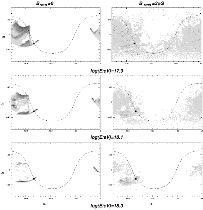
Figure 1: Arrival direction distribution in celestial coordinates for increasing values of the CR energy. In the left panels only the regular galactic magnetic field is included while in the right panel a random field component with $B_{rms}=3~{}\mu G$ is included. The dashed line represents the galactic plane with the black dot in it corresponding to the direct neutron flux from the GC. Darker points correspond to greater density in logarithmic scale.

when only the regular magnetic field component is included and for different values of the energy between $10^{17.9}$ eV and $10^{18.3}$ eV. The most intense flux arrives from the GC direction ($\alpha_{GC}=266.4^{\circ}$ and $\delta_{GC}=-28.9^{\circ}$) and corresponds to the direct neutrons. A thin (nearly horizontal) strip extending from the GC towards the north and south galactic poles (i.e. perpendicular to the galactic plane, shown as a dashed line) is due to neutrons decaying near the Earth in our spiral arm and in the nearest inner arm respectively. The more extended excess appearing for right ascensions between $300^{\circ}$ and $360^{\circ}$ correspond to neutrons that decayed in the inner galactic region, with the protons reaching the Earth through the spiral arm. We can see that the region of the sky where events are spread shrinks considerably with increasing energy, in particular, at $10^{18.3}$ eV almost all the events arrive outside the field of vision of AGASA ($\delta>-24^{\circ}$). Notice that the flux intensity of the plots with different energy should not be compared at this point, as the energy spectrum of the source has not yet been introduced.

The inclusion of the turbulent magnetic field component leads to a spreading in the arrival direction distribution as illustrated in the right panels of Figure 1, in which $B_{rms}=3~{}\mu$G was adopted. The spread in the arrival directions increases with the strength of the random component, as indicated by Equation (4), and this is clearly seen in the left panels of Figure 2, which show this distribution for a fixed energy of $10^{18}$ eV and increasing intensity of the random field ($B_{rms}=0,1,2$ and $3~{}\mu$G).

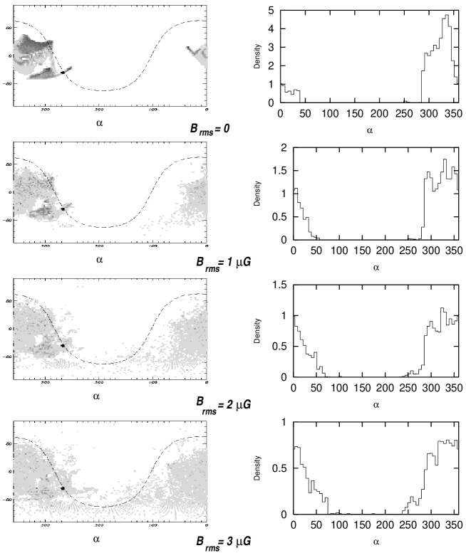
Figure 2: The left panels show the arrival direction distribution in celestial coordinates for different values of turbulent field strength $B_{rms}=0,1,2$ and $3~{}\mu$G. In all plots the energy is $E=1$ EeV. The right panels show the corresponding right ascension distribution taking into account the AGASA exposure.

The right ascension density distribution for the $B_{rms}=3~{}\mu$G random field maps of Figure 1 is shown in the left panels of Figure 3.

Figure 3: Right ascension density distribution corresponding to the a random field with $B_{rms}=3~{}\mu G$ for different values of the CR energy. The left panels are for the full sky maps, while in the right panels the exposure of AGASA is used. The scale is in arbitrary units.

The sharp peak in $\alpha\sim 265^{\circ}$ is mainly due to the direct neutrons. This is relatively more important as the energy is increased, due to the increase in the neutron’s decay length. The broader excess associated to the secondary protons arriving along the spiral arm becomes strongly suppressed above $10^{18}$ eV due to the increasing difficulty for the regular field to confine the CRs along the spiral arms. This suppression is clearly expected to be more important as the value of $B_{rms}$ becomes stronger, while on the other hand a larger value of the regular component $B_{0}$ should lead to a signal more concentrated in the spiral arm direction and surviving up to larger energies.

In order to compare our results with AGASA’s measurements, it is necessary to take into account the exposure ($\omega$) of the observatory, which gives the time-integrated effective collecting area from each direction of the celestial sphere. The arrival direction distribution measured by an observatory should be proportional to the actual distribution multiplied by $\omega$.

The exposure is expected to be homogeneous in right ascension ($\alpha$) and to have a declination ($\delta$) dependence given by [13]

$$\omega(\delta)\propto\cos(a_{0})\cos(\delta)\sin(\alpha_{m})\ +\alpha_{m}\sin(a_{0})\sin(\delta),$$ (5)

where $\alpha_{m}$ is given by

$$\alpha_{m}=\left\{\begin{array}[]{ll}0&\textrm{if $\xi>1$}\\ \pi&\textrm{if $\xi<-1$}\\ \cos^{-1}(\xi)&\textrm{otherwise}\end{array}\right.$$ (9)

and

$$\xi\equiv\frac{\cos(\theta_{m})-\sin(a_{0})\sin(\delta)}{\cos(a_{0})\cos(\delta)},$$

where $a_{0}$ is the detector latitude (in the case of AGASA $a_{0}=35.78^{\circ}$) and $\theta_{m}$ is the maximum zenith angle observed. The analysis of AGASA data correspond to events with zenith angle $\theta<60^{\circ}$.

Taking into account the exposure, the right ascension distribution expected to be measured at the AGASA latitude looks as shown in the right panels of Figure 3 for a random field amplitude $B_{rms}=3~{}\mu$G. The main difference with the full sky results displayed in the left hand panels is the disappearance of the point-like density peak due to the direct neutrons. The right panels of Figure 2 also show this distribution for different values of $B_{rms}$ and for $E=10^{18}$eV, for the AGASA exposure. The increasing spread of the signal associated to the spiral arm, which is the dominating one in this case, is apparent.

Anisotropies in the CR distribution are often measured performing an harmonic analysis of the right ascension distribution of the events [17]. This takes advantage of the uniform exposure in right ascension of most experiments. The right ascension distribution is related to the differential spectrum of CR, ${\rm d}J/{\rm d}\Omega(E)$ through

$$F(\alpha)=\int{\rm d}\delta\cos\delta\omega(\delta)\frac{{\rm d}J}{{\rm d}\Omega}.$$

Expanding it as $F(\alpha)=F_{0}+F_{1}\cos(\alpha-\alpha_{1})+\dots,$ the amplitude of the anisotropy is defined as the ratio of the dipole to the monopole intensities: $\Delta\equiv F_{1}/F_{0}$. In Table 1, the phase of the first harmonic ($\alpha_{1}$)

Table 1: Phases of the first harmonic from the analysis of the right ascension distribution as a function of energy and turbulent magnetic field strength, for the exposure at the AGASA latitude and at $35^{\circ}$ south.

• $B_{rms}$	log(E)	AGASA	SOUTH
  0 $\mu$G		328	302
  1 $\mu$G	18.0	333	303
  2 $\mu$G		339	301
  3 $\mu$G		341	298
  	17.9	340	308
  3 $\mu$G	18.1	344	291
  	18.2	354	286
  	18.3	358	279

from the analysis of the right ascension distribution are listed as a function of energy and turbulent magnetic field strength, taking into account AGASA’s exposure, and also for a hypotetical detector in the southern hemisphere (at a latitude $-35^{\circ}$, similar to the one of AUGER or Sidney).

3.2 Amplification

The total flux that we receive from a given source is modified by the presence of a magnetic field. This can be described by introducing the amplification, $A(E)$, which is the ratio of the flux of particles arriving to the Earth from any direction in the presence of the GMF, $J(E)$, and that in the absence of magnetic field, $J_{0}(E)$, i. e. $A(E)=J(E)/J_{0}(E)$. The amplification is a function of the energy and the mean effect turns out to be larger as the energy decreases, as expected since the CRs tend to be trapped more efficiently in the spiral arms of the GMF. At larger energies the amplification tends to unity, as protons are less affected by the magnetic field and a larger fraction of the neutrons arrive to the Earth before decaying. Figure 4 shows the amplification vs. energy for adopted values of the random magnetic field of $B_{rms}=0$ and $3~{}\mu$G. The smaller amplification obtained in the presence of the random magnetic field is due to the enhancement of the escape of CRs from the spiral arms produced by this component.

Figure 4: Amplification vs. energy of a neutron source located at the GC due to the GMF, with (solid line) and without (dotted line) including the turbulent component of the GMF ($B_{rms}=3\ \mu$G) in the simulation.

3.3 Anisotropy

The anisotropy detected by AGASA arises in a narrow range of energies from $E=10^{17.9}$eV to $E=10^{18.3}$eV. It has been suggested that the lack of anisotropies at smaller energies could be explained in the model discussed here because of the shorter decay length of the neutrons and the deflection of the resulting protons in the galactic magnetic field. In order to test quantitatively this hypothesis we have to estimate the total anisotropy produced by the GC neutron source in the presence of the background of all the other sources of CR in that energy range.

The flux of CRs with energy around 1 EeV arriving to the Earth is thought to come from galactic sources, such as supernovae, that give the main contribution below the ankle ($E_{ankle}\simeq 5\times 10^{18}$ eV), as well as extragalactic sources, which dominate above the ankle. This can be splitted into the flux from the GC source, ${\rm d}J/{\rm d}\Omega(E)$, and the contribution from all the other sources, ${\rm d}J_{bkg}/{\rm d}\Omega(E)$, i.e. ${\rm d}J_{tot}/{\rm d}\Omega={\rm d}J_{bkg}/{\rm d}\Omega+{\rm d}J/{\rm d}\Omega$.

The total (measured) differential energy spectrum of CRs can be approximated by [18]

$$\frac{{\rm d}J_{tot}}{{\rm d}\Omega}(E)=C\times\bigg{(}\frac{E}{6.3\times 10^{18}}\bigg{)}^{-3.2\pm 0.05}$$ (10)

in the range of energies from $4\times 10^{17}\ \mathrm{eV}<E<6.3\times 10^{18}\ \mathrm{eV}$, and $C=(9.23\pm 0.65)\times 10^{-33}\mathrm{m}^{-2}\mathrm{s}^{-1}\mathrm{sr}^{-1}\mathrm{eV}^{-1}$.

The intensity of the total flux received at the Earth from the source is $J(E)=J_{0}(E)A(E)$, where $A(E)$ is the amplification computed in the previous section and for the actual source flux we can consider a power law dependence with energy $J_{0}(E)\propto E^{-2.2}$, which is typical of Fermi acceleration in shocks.

If we assume that the main contribution to the anisotropy comes from the GC neutron source, and hence consider that the background CR flux is essentially isotropic, we can write the observed anisotropy as $\Delta(E)=\Delta_{s}(E)f(E)$, where $f(E)\equiv F_{0(s)}/F_{0(bkg)}$ is the ratio of the contributions to the right ascension monopole from the source flux and the background flux. For an anisotropic flux, as in this case, $f(E)$ depends on the exposure of the experiment. The anisotropy of the source flux, $\Delta_{s}(E)$, can be computed from the harmonic analysis of the right ascension distribution of the GC events as discussed in Section 3.1. We show in Figure 5 the expected anisotropy as a function of the energy for different values of the turbulent magnetic field amplitude and exposures.

Figure 5: Anisotropy as a function of energy for random magnetic fields of strengths $B_{rms}=1$ and $3~{}\mu$G, and for exposures corresponding to full sky (FS), AGASA (AG) and for a southern observatory at $b=-35^{\circ}$ (S).

For a random field amplitude $B_{rms}=3~{}\mu$G, the anisotropy grows sharply around $E=10^{17.8}$ as observed by AGASA. This is not the case for smaller values of the rms amplitude of the turbulent field as is apparent from the curve labeled $B_{rms}=1~{}\mu$G in the Figure, as the CR arrival directions are not spread sufficiently at small energies to wash out the anisotropies. Notice that the effects associated to a harder GC source spectrum are partially compensated by the effects due to the increased amplification of the fluxes for decreasing energies, leading to a more moderate energy dependence. We have normalized the source flux in such a way that the anisotropy is 4$\%$ at $E\simeq 10^{18}$eV for the AGASA exposure. This corresponds to a fraction $f\simeq 0.026$ contributed by the GC source to the right ascension monopole at that energy.

The sharp fall in the anisotropy appearing at $E\simeq 10^{18.3}$ eV for the AGASA curve arises because above that energy most CRs arrive as direct neutrons from the GC direction, which is out of the field of view of AGASA. The possible existence of a cutoff in the acceleration energy of the source around that range of values is actually not necessary to explain AGASA’s results.

3.4 Source luminosity

We can estimate the luminosity of the GC source which corresponds to the normalization of its flux at the Earth adopted in the previous Section to fit the 4$\%$ amplitude of the right ascension first harmonic measured by AGASA. This is given by

$$L_{GC}=4\pi r_{0}^{2}\int\mathrm{d}EEJ_{0}(E),$$ (11)

where $r_{0}$ is the distance to the GC, and the source flux in the absence of magnetic fields is given by $J_{0}(E)=J(E)/A(E)$. The source flux $J(E)$ at $10^{18}$eV can be related to the background flux $J_{bkg}$ at that energy using the value of $f(E)$ obtained in the last Section. With the amplification computed in Section 3.2, the local flux at $10^{18}$eV results $J_{0}(10^{18}~{}{\rm eV})\simeq 1.3\times 10^{-30}m^{-2}s^{-1}{\rm eV}^{-1}$. For a power law energy spectrum of the source $J_{0}(E)\propto E^{-2.2}$, the total luminosity in the decade of energy from $10^{17.5}$ to $10^{18.5}$ then results $L_{GC}(10^{17.5}-10^{18.5})\simeq 4\times 10^{36}$ erg/s. This value is more than an order of magnitude lower than the maximum luminosity ($10^{38}$ erg/s) estimated for Sgr A* [8] mentioned in the Introduction.

The expected flux of direct neutrons is a factor $e^{-r_{0}/\gamma c\tau_{n}}$ of the source flux $J_{0}(E)$. The integral of this in the energy range from $10^{17.9}$ eV to $10^{18.5}$ eV corresponds then to a direct neutron flux of $2\times 10^{-13}{\rm m}^{-2}s^{-1}$, which is not very different from the value $(9\pm 3)\times 10^{-14}{\rm m}^{-2}{\rm s}^{-1}$ reported by SUGAR for their point-like excess [4].

In order to give an idea of the distribution of the excess of events over the ones expected for an isotropic distribution, we made a map (similar to those constructed by AGASA and SUGAR) in which we added to an isotropic background the CR density expected from a GC neutron source of the required intensity to fit the AGASA’s right ascension anisotropy. The map in Figure 6 displays the ratio of the intensity at each direction to the mean density at that declination (following AGASA’s analysis). We have smoothed the map with a window of $3^{\circ}$ radius to take into account the typical angular resolution at these energies. Although the particular details of the map will depend on the GMF structure and strength, that are poorly known, we think that the main characteristic of the distribution are picked with the realistic model adopted. Notice however that the proton signal around the GC is sensitive to the actual location of the reversals in direction of the regular magnetic field. In the model adopted, in which the nearest reversal to the GC direction is at less than 1 kpc from the Earth, the excess observed at southern galactic latitudes is more significant than the one at northern latitudes, but this could change if the reversal was at a smaller galactocentric radius. Also, a vertical component of the magnetic field could displace these excesses in the direction parallel to the galactic plane.

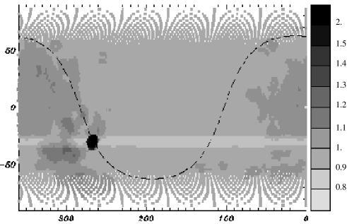
Figure 6: Ratio of the density in each direction to the mean density at that declination for $E=1$ EeV and $B_{rms}=3\ \mu$G.

4 Conclusions

We examined the possibility that a source of neutrons at the GC could be responsible for the anisotropy measured by AGASA and SUGAR. As the GC itself is out of the field of view of AGASA, this observatory would not detect direct neutrons from a source in the GC, but it would just see the protons produced by the neutron decays. As their trajectories are bent by the GMF, the distribution of protons arriving to the Earth depends strongly on the energy of the particles and on the structure and strength of the field, which are not well known. We assumed a particular model for the regular field, which is consistent with the main observational evidences, and considered different reasonable amplitudes for the turbulent magnetic field. We found that there is a sharp rise in the anisotropy at energies around 1 EeV, as observed by AGASA, for the largest amplitude of the turbulent magnetic field considered, $B_{rms}=3~{}\mu$G. At energies larger than 2 EeV, essentially no particles are expected from the GC source in the field of view of AGASA, what explains the disappearance of the anisotropy independently of the source acceleration cutoff. The predictions are however very different for an observatory in the south. This one should detect the strong point-like signal from the direct neutrons in addition to the extended signal from the protons. At energies below 1 EeV the neutron signal is suppressed due to the reduced decay length of the neutrons and the expected anisotropy has a similar behavior as that of a northern observatory. At larger energies, and up to the maximum acceleration energy of the source, the point-like signal should be clearly seen. It is interesting to notice that the neutron source luminosity needed to fit the $4\%$ right ascension anisotropy detected by AGASA (due to the protons in this model) give rise to a point-like neutron flux consistent with the one measured by SUGAR. However, unless there is some systematic pointing error in their data, the offset of the signal from the GC direction cannot be explained. Moreover, for the GMF adopted, the phase of the first harmonic in right ascension obtained ($\sim 330^{\circ}$) is somewhat larger than AGASA’s one. Another important point is that within this scenario the excess observed along the Cygnus region is also related to the central source (for this it is crucial that the regular magnetic field be along the spiral arm and not just azimuthal). This excess disappears for $E>2\times 10^{18}$ eV due to the impossibility for the GMF to confine the CRs along the spiral arms, independently of the source upper energy cutoff. The alternative explanation of a diffusive flux of charged particles from the GC direction [9, 10] should give rise to a wide angle anisotropy, with a deficit of particles in the galactic anticenter direction and a cosine angular dependence with respect to the direction of maximum flux, quite different from the neutron source signal. More data from an observatory in the south would be very helpful to confirm or reject these hypothesis. Although the AUGER observatory [19] in construction in Argentina is focused to the study of CRs with energy above $10^{19}$ eV, it may be able to detect lower energy events (down to $10^{18}$ eV). A dedicated detector for the $10^{17}$ eV to $10^{19}$ eV energy range is also under study [20].

If the sharp peak in the GC direction is seen, confirming the neutron source hypothesis, then the distribution of the protons would give information about the structure of the GMF.

References

References

- [1] Hillas A M 1984 An. Rev. Astron. Astrophys. 22 425
- [2] Hayashida N et al. 1999 Astropart. Phys. 10 303
- [3] Hayashida N et al. 1999 Proceedings of 26th ICRC (Salt Lake City) and astro-ph/9906056
- [4] Bellido J A, Clay R W, Dawson B R and Johnston-Hollitt M 2001 Astropart. Phys. 15 167
- [5] Berezinskii V S and Prilutskii O F 1977 Sov. Astron. Lett. 3 141
- [6] Medina-Tanco G A and Watson A A 2001 Proceedings of ICRC 2001 (Hamburg) 531
- [7] Nagataki S and Takahashi K, astro-ph/0108507
- [8] Levinson A and Boldt E 2002 Astropart. Phys. 16 265
- [9] Teshima M et al. 2001 Proceedings of ICRC 2001 (Hamburg) 337
- [10] Candia J, Mollerach S and Roulet E 2002 J. High Energy Phys. JHEP12(2002)032
- [11] Clay R W, Dawson B R, Bowen J and Debes M 2000 Astropart. Phys. 12 249
- [12] Bednarek W, Giller M and Zielinska M 2002 J. Phys. G 28 2283
- [13] Sommers P 2001, Astropart. Phys. 14 271
- [14] Harari D, Mollerach S and Roulet E 1999 J. High Energy Phys. JHEP08(1999)022
- [15] Stanev T 1997 Astrophys. J. 479 290
- [16] Harari D, Mollerach S, Roulet E and Sánchez F 2002 J. High Energy Phys. JHEP03(2002)045
- [17] Linsley J 1975 Phys. Rev. Lett. 34 1530
- [18] Nagano M and Watson A A 2000 Rev. of Mod. Phys. 72 689
- [19] Auger Collaboration (1997) The Pierre Auger Observatory Design Report, Second edition (http://www.auger.org)
- [20] Adams T, Loh E C, BenZvi S and Westerhoff S 2003, astro-ph/0303484