Continuous Limit of Multiple Gravitational Lens Effect and Average Magnification Factor

Abstract

We show that the gravitational magnification factor averaged over all configurations of lenses in a locally inhomogeneous universe satisfy a second order differential equation with redshift $z$ by taking the continuous limit of multi-plane gravitational lens equation (the number $N_{\mathrm{L}}$ of lenses $\to\infty$) and that the gravitationally magnified Dyer-Roeder distance in a clumpy universe becomes to that of the Friedmann-Lemaître universe for arbitrary values of the density parameter $\Omega_{0}$ and of a mass fraction $\bar{\alpha}$ (smoothness parameter).

1 Introduction

A light ray propagation in a locally inhomogeneous universe has been investigated by many authors using analytical and/or numerical methods (e.g., Omote & Yoshida 1990; Yoshida & Omote 1992;Schneider, Ehlers & Falco 1992, and references therein). By taking gravitational lens effects into account, Weinberg (1976) showed that in a case of the low deacceleration parameter $q_{0}=\Omega_{0}/2-\lambda_{0}$ ($\Omega_{0},\lambda_{0}$ are the density parameter and the cosmological constant, respectively) an average flux from sources in a clumpy universe is equal to the flux in the Friedmann-Lemaître universe (flux conservation). For a more general value of $\Omega_{0}$, some authors (e.g., Ehlers & Schneider, 1986; Peacock, 1986) discussed the gravitational magnification probability function by assuming the flux conservation.

Recent observations on high-redshift Type Ia supernovae (Perlmutter et al., 1999) and on the cosmic microwave background (CMB, Spergel et al., 2003) suggest that our universe is accelerating in expansion rate. In such a situation, the deacceleration parameter may be no longer small. Then it is needed to consider the light ray propagation in a more general inhomogeneous universe model with arbitrary values of $\Omega_{0}$ and $\lambda_{0}$ for sources with high-redshifts.

In a case with an arbitrary $\Omega_{0}$, we have to take magnification effects by multiple lenses into account. In studies of this problem the multi-plane lens theory has been used both in analytical approximations (Peacock, 1986; Isaacson & Canizares, 1989; Schneider & Weiss, 1988a; Wu, 1990; Marchandon & Nottale, 1991; Seitz & Schneider, 1994) and in numerical simulations (Refsdal 1970; Schneider & Weiss 1988b; Watanabe & Tomita 1990; Rauch 1990; Lee, Babul, Kofman & Kaiser 1997; Premadi, Martel, Matzner & Futamase 2001). In analytical studies many authors (Vietri & Ostriker, 1983; Pei, 1993; Schneider, 1993) have assumed that the total magnification by lenses can be approximately given by a product of the magnifications of individual lens, and have obtained statistically the total magnification by gravitational lenses distributed at random in the universe.

In this paper we consider the total gravitational magnification factor averaged with all configurations of lenses distributed at random in a locally inhomogeneous universe and discuss the continuous limit (the number $N_{\mathrm{L}}$ of lens planes $\to\infty$) in which lens planes approach to be continuously distributed. In §2 the multi-plane lens theory is briefly reviewed and an average magnification matrix is obtained in §3. In §4 the continuous limit of the magnification matrix is considered. We show that in this limit the average magnification factor satisfies a second order differential equation and that a angular diameter distance multiplied by $\left<\mu(z)\right>^{-1/2}$ ($\left<\mu(z)\right>$: average magnification factor) reduces to the angular diameter distance of the homogeneous universe (the Friedmann–Lemaître universe).

2 Multi-plane lens equation

We will give a brief review of the multi-plane lens equation in this section. Suppose that $N_{\mathrm{L}}$ lenses are randomly distributed at redshifts $z_{i}(0\leq z_{1}<z_{2}\cdots<z_{N_{\mathrm{L}}})$, and that $z_{\mathrm{S}}=z_{N_{\mathrm{L}}+1}>z_{N_{\mathrm{L}}}$ is a redshift of the source (see Fig. 1).

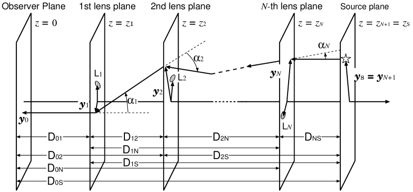
Figure 1: Geometry of multi-plane lens system: $\mathrm{L}_{i}$ is the $i$-th lens. Each lens plane is perpendicular to observer’s line of sight. The origin of each lens plane is set on the line of sight. The light ray observed at $\mbox{\boldmath$y$}_{0}$ in the observer plane crosses at $\mbox{\boldmath$y$}_{i}$ in the $i$-th lens plane. $D_{ij}$ denotes the angular diameter distance from the $i$-th lens plane to the $j$-th lens plane (the observer is in the the $0$-th lens plane and the source is in the ($N+1$)-th lens plane).

The multi-plane lens equation for the source is given by

$$\mbox{\boldmath$y$}_{\mathrm{S}}={D(0;z_{\mathrm{S}})\over D(0;z_{1})}\mbox{\boldmath$y$}_{1}-\sum_{i=1}^{N_{\mathrm{L}}}D(z_{i};z_{\mathrm{S}})\mbox{\boldmath$\alpha$}_{i}(\mbox{\boldmath$y$}_{i}),$$ (1)

where $\mbox{\boldmath$y$}_{\mathrm{S}}$ denotes the position vector of the source at the source plane and $\mbox{\boldmath$y$}_{i}$ is the position vector of the light ray at the $i$-th lens plane (Schneider et al., 1992). In equation (1) $D(z_{i};z_{j})$ is the angular diameter distance from the $i$-th lens plane at $z_{i}$ to the $j$-th lens plane at $z_{j}$. The deflection angle $\mbox{\boldmath$\alpha$}_{i}(\mbox{\boldmath$y$}_{i})$ at the $i$-th lens plane is given by

$$\mbox{\boldmath$\alpha$}_{i}(\mbox{\boldmath$y$}_{i})={4G\over c^{2}}\int\!\!\!\!\int_{{\cal S}_{i}}d^{2}\mbox{\boldmath$y$}_{i}^{\prime}\Sigma_{i}(\mbox{\boldmath$y$}_{i}^{\prime}){\mbox{\boldmath$y$}_{i}-\mbox{\boldmath$y$}_{i}^{\prime}\over|\mbox{\boldmath$y$}_{i}-\mbox{\boldmath$y$}^{\prime}_{i}|^{2}},$$ (2)

where $\Sigma_{i}(\mbox{\boldmath$y$}_{i}^{\prime})$ is a surface mass density of the $i$-th lens and ${\cal S}_{i}$ denotes the observed region on the $i$-th lens plane.

We should notice that an image at $\mbox{\boldmath$y$}_{i}$ on the $i$-th lens plane could be regarded as a “source” by the foreground lenses. Therefore the multi-plane lens equation for the “source” at $\mbox{\boldmath$y$}_{i}$ can be rewritten as follows:

$$\mbox{\boldmath$y$}_{i}={D(0;z_{i})\over D(0;z_{1})}\mbox{\boldmath$y$}_{1}-\sum_{j=1}^{i}D(z_{j};z_{i})\mbox{\boldmath$\alpha$}_{j}(\mbox{\boldmath$y$}_{j}).$$ (3)

In the following we use new variables $\mbox{\boldmath$\theta$}_{i}=\mbox{\boldmath$y$}_{i}/D(0;z_{i})\ (i=1,\cdots,N_{\mathrm{L}}+1=\mathrm{S})$ which denote the angular position of the light ray in the $i$-th lens plane. Using a dimensionless angular diameter distance $d(z_{i};z_{j})=D(z_{i};z_{j})/(c/H_{0})$, we can rewrite equation (3) as follows:

$$\mbox{\boldmath$\theta$}_{i}=\mbox{\boldmath$\theta$}_{1}-\sum_{j=1}^{i}{d(z_{j};z_{i})\over d(0;z_{i})}\mbox{\boldmath$\alpha$}_{j}[D(0;z_{j})\mbox{\boldmath$\theta$}_{j}].$$ (4)

Using the $\chi$-function introduced by Schneider et al. (see equation [A8] in Appendix A), the distance $d(z_{j};z_{i})$ from the $j$-th lens plane to the $i$-th lens plane is given by $d(z_{j};z_{i})=(1+z_{j})d(0;z_{j})d(0;z_{i})(\chi_{j}-\chi_{i})$, then equation (4) is rewritten in the following expression

$$\mbox{\boldmath$\theta$}_{i}=\mbox{\boldmath$\theta$}_{i-1}-(\chi_{i-1}-\chi_{i})\sum_{j=1}^{i-1}(1+z_{j})\tilde{\mbox{\boldmath$\alpha$}}_{j}(\mbox{\boldmath$\theta$}_{j}),$$ (5)

where

$$\tilde{\mbox{\boldmath$\alpha$}}_{j}(\mbox{\boldmath$\theta$}_{j})=d(0;z_{j})\mbox{\boldmath$\alpha$}_{j}[D(0;z_{j})\mbox{\boldmath$\theta$}_{j}]={4G\over cH_{0}}d^{2}(0;z_{j})\int\!\!\!\!\int_{{\cal D}}d^{2}\mbox{\boldmath$\theta$}_{j}^{\prime}\Sigma_{j}[D(0;z_{j})\mbox{\boldmath$\theta$}_{j}^{\prime}]{\partial\ \over\partial\mbox{\boldmath$\theta$}_{j}}\ln|\mbox{\boldmath$\theta$}_{j}-\mbox{\boldmath$\theta$}_{j}^{\prime}|,$$ (6)

and $\mbox{\boldmath$\theta$}^{\prime}_{j}$ and ${\cal D}$ denote the angular coordinate on the $j$-th lens plane and the observed region, respectively. An expression similar to equation (5) has been given by Petters, Levine & Wambsganss (2001). This recurrence formula (5) determines iteratively the “source” position $\mbox{\boldmath$\theta$}_{i}$ in terms of $\mbox{\boldmath$\theta$}_{j}(j<i)$ and is useful in a numerical experiment based on the ray tracing method. An equivalent equation to equation (1) can be also obtained from the Fermat principle (Blandford & Narayan, 1986; Kovner, 1987):

$$\chi_{i,i+1}\left(\mbox{\boldmath$\theta$}_{i+1}-\mbox{\boldmath$\theta$}_{i}\right)=\chi_{i-1,i}\left(\mbox{\boldmath$\theta$}_{i}-\mbox{\boldmath$\theta$}_{i-1}\right)-(1+z_{i})\tilde{\mbox{\boldmath$\alpha$}}_{i}(\mbox{\boldmath$\theta$}_{i}),$$ (7)

where $\chi_{i,j}=[\chi_{i}-\chi_{j}]^{-1}$.

Now we give the magnification matrix $A_{\mathrm{S},N_{\mathrm{L}}}$ in the case of the multi-plane lensing by using equation (1) and (4) as

$$A_{\mathrm{S},N_{\mathrm{L}}}\equiv{\partial\mbox{\boldmath$\theta$}_{\mathrm{S}}\over\partial\mbox{\boldmath$\theta$}_{1}}=I-\sum_{i=1}^{N_{\mathrm{L}}}{(1+z_{i})\over\chi_{i,\mathrm{S}}}\tilde{U_{i}}A_{i},$$ (8)

where $I$ is the $2\times 2$ unit matrix and $\tilde{U}_{i}$ and $A_{i}$ are matrices defined by

$$\tilde{U}_{i}\equiv{\partial\tilde{\mbox{\boldmath$\alpha$}}_{i}\over\partial\mbox{\boldmath$\theta$}_{i}},\quad A_{i}\equiv{\partial\mbox{\boldmath$\theta$}_{i}\over\partial\mbox{\boldmath$\theta$}_{1}}.$$ (9)

We should notice that $\tilde{U}_{i}$ defined in terms of $\tilde{\mbox{\boldmath$\alpha$}}_{i}$ is slightly different from the matrix $U_{i}$ $(\equiv\partial\mbox{\boldmath$\alpha$}_{i}/\partial\mbox{\boldmath$\theta$}_{i})$ in Schneider et al. (1992). While $U_{i}$ in their definition depends on the redshift $z_{\mathrm{S}}$ of the source, $\tilde{U}_{i}$ in our definition does not since $\tilde{\mbox{\boldmath$\alpha$}}_{i}$ is independent of $z_{\mathrm{S}}$. By virtue of equations (4), (8) and (9), we obtain the following form:

$$A_{\mathrm{S},N_{\mathrm{L}}}=I+\sum_{k=1}^{N_{\mathrm{L}}}(-)^{k}\sum_{i_{1}=1}^{i_{0}}\sum_{i_{2}=1}^{i_{1}}\cdots\sum_{i_{k}=1}^{i_{k-1}}{(1+z_{i_{1}})(1+z_{i_{2}})\cdots(1+z_{i_{k}})\over\chi_{i_{k},i_{k-1}}\cdots\chi_{i_{2},i_{1}}\chi_{i_{1},i_{0}}}\tilde{U}_{i_{1}}\tilde{U}_{i_{2}}\cdots\tilde{U}_{i_{k}},$$ (10)

where $i_{0}~{}(=N_{\mathrm{L}}+1)>i_{1}>i_{2}>\cdots>i_{k-1}>i_{k}\geq 1$, and the matrix $\tilde{U}_{i}$ can be expressed as

$$\tilde{U}_{i}(\mbox{\boldmath$\theta$}_{i}) = {4G\over cH_{0}}d^{2}(0;z_{i})\int\!\!\!\!\int_{{\cal D}}d^{2}\mbox{\boldmath$\theta$}^{\prime}\Sigma_{i}[D(0;z_{i})\mbox{\boldmath$\theta$}^{\prime}]\tilde{U}_{i}^{\prime}(\mbox{\boldmath$\theta$}_{i}-\mbox{\boldmath$\theta$}^{\prime}),$$ (11)

$$\tilde{U}_{i}^{\prime}(\mbox{\boldmath$\eta$}) = \left(\begin{array}[]{cc}\pi\delta^{2}(\mbox{\boldmath$\eta$})-\Gamma_{1}(\mbox{\boldmath$\eta$})&-\Gamma_{2}(\mbox{\boldmath$\eta$})\\ -\Gamma_{2}(\mbox{\boldmath$\eta$})&\pi\delta^{2}(\mbox{\boldmath$\eta$})+\Gamma_{1}(\mbox{\boldmath$\eta$})\\ \end{array}\right),$$ (14)

and

$$\Gamma_{1}(\mbox{\boldmath$\eta$})={\eta_{x}^{2}-\eta_{y}^{2}\over|\mbox{\boldmath$\eta$}|^{4}},\quad\Gamma_{2}(\mbox{\boldmath$\eta$})={2\eta_{x}\eta_{y}\over|\mbox{\boldmath$\eta$}|^{4}}.$$ (15)

Recurrence formulae of the magnification matrix given by equation (5) or (7) are also written as:

$$A_{i}=A_{i-1}-\frac{1}{\chi_{i-1,i}}\sum_{j=1}^{i-1}(1+z_{j})\tilde{U}_{j}A_{j},$$ (16)

$$\chi_{i,i+1}\left(A_{i+1}-A_{i}\right)=\chi_{i-1,i}\left(A_{i}-A_{i-1}\right)-(1+z_{i})\tilde{U}_{i}A_{i}.$$ (17)

3 Average Magnification Matrix

In this section the universe is assumed to be a locally inhomogeneous, on-average homogeneous and isotropic universe in which a mass fraction $\bar{\alpha}$ (smoothness parameter) of the mean matter density $\bar{\rho}(z)$ is smoothly distributed, while a fraction $(1-\bar{\alpha})\bar{\rho}(z)$ is concentrated into clumps distributed at random. The angular diameter distance $D(z;z^{\prime})$ of this universe from a redshift $z$ to another redshift $z^{\prime}$ satisfies the Dyer–Roeder equation (A6) with $0\leq\bar{\alpha}<1$ (Dyer & Roeder, 1973).

In this universe a light ray passes through the space with the smoothly distributed mass density $\bar{\alpha}\bar{\rho}(z)$ and is gravitationally affected several times by clumps (lenses) located near the light path, in general. Since the gravitational magnification factor for the light ray depends on the distribution of lenses near the light path, we cannot discuss the individual gravitational magnification factor of a source without the knowledge about the configuration of lenses near the light ray from the source. Nevertheless it is meaningful to estimate an average gravitational magnification factor for light rays which travel in various regions of the inhomogeneous universe, because the factor plays an important role in the theoretical analysis of observed data such as $m-z$ relation.

In the following we consider only the gravitational magnification factor $\left<\mu\right>=\det\left<A_{\mathrm{S},N_{\mathrm{L}}}\right>^{-1}$ averaged over all distributions $\{\mbox{\boldmath$\xi$}_{1},\cdots,\mbox{\boldmath$\xi$}_{N_{\mathrm{L}}}\}$ of lenses on each lens plane ($\mbox{\boldmath$\xi$}_{i}$: center of the $i$-th lens) in the locally inhomogeneous universe defined by

$$\left<A_{\mathrm{S},N_{\mathrm{L}}}\right> \equiv {\int\!\!\!\!\int_{\cal D}d^{2}\mbox{\boldmath$\xi$}_{1}\cdots\int\!\!\!\!\int_{\cal D}}d^{2}\mbox{\boldmath$\xi$}_{N_{\mathrm{L}}}A_{\mathrm{S},N_{\mathrm{L}}}(\mbox{\boldmath$\xi$}_{1},\cdots,\mbox{\boldmath$\xi$}_{N_{\mathrm{L}}})\biggl{/}{\int\!\!\!\!\int_{\cal D}d^{2}\mbox{\boldmath$\xi$}_{1}\cdots\int\!\!\!\!\int_{\cal D}}d^{2}\mbox{\boldmath$\xi$}_{N_{\mathrm{L}}}$$ (18)

$$= Q^{-N_{\mathrm{L}}}\int\!\!\!\!\int_{\cal D}d^{2}\mbox{\boldmath$\xi$}_{1}\cdots\int\!\!\!\!\int_{\cal D}d^{2}\mbox{\boldmath$\xi$}_{N_{\mathrm{L}}}A_{\mathrm{S},N_{\mathrm{L}}}(\mbox{\boldmath$\xi$}_{1},\cdots,\mbox{\boldmath$\xi$}_{N_{\mathrm{L}}}),$$

where $Q$ is the solid angle of the observed region $\cal D$. Here it should be noticed that to take all configurations of lenses into account means to consider observed regions in various directions as well as various lens distributions on the individual lens plane. By virtue of equation (10) the average magnification matrix is given by

$$\left<A_{\mathrm{S},N_{\mathrm{L}}}\right> = I+\sum_{k=1}^{N_{\mathrm{L}}}(-)^{k}\sum_{i_{1}=1}^{i_{0}}\sum_{i_{2}=1}^{i_{1}}\cdots\sum_{i_{k}=1}^{i_{k-1}}{(1+z_{i_{k}})\cdots(1+z_{i_{2}})(1+z_{i_{1}})\over\chi_{i_{k},i_{k-1}}\cdots\chi_{i_{2},i_{1}}\chi_{i_{1},i_{0}}}$$ (19)

$$\hskip 56.9055pt\times\left<\tilde{U}_{i_{1}}(\mbox{\boldmath$\xi$}_{i_{1}};\mbox{\boldmath$\theta$}_{i_{1}})\tilde{U}_{i_{2}}(\mbox{\boldmath$\xi$}_{i_{2}};\mbox{\boldmath$\theta$}_{i_{2}})\cdots\tilde{U}_{i_{k}}(\mbox{\boldmath$\xi$}_{i_{k}};\mbox{\boldmath$\theta$}_{i_{k}})\right>,$$

where $\tilde{U}_{i}(\mbox{\boldmath$\xi$}_{i};\mbox{\boldmath$\theta$}_{i})$ denotes the matrix for the $i$-th lens centered on $\mbox{\boldmath$\xi$}_{i}$ given by equation (11).

As shown in Appendix B, if the lenses are distributed at random in the universe, i.e., if they does not correlate each other, the average of the product of matrices $\tilde{U}_{i}$ reduces to the product of the average matrices $\left<\tilde{U}_{i}\right>$, i.e.,

$$\left<\tilde{U}_{i_{1}}(\mbox{\boldmath$\xi$}_{i_{1}};\mbox{\boldmath$\theta$}_{i_{1}})\tilde{U}_{i_{2}}(\mbox{\boldmath$\xi$}_{i_{2}};\mbox{\boldmath$\theta$}_{i_{2}})\cdots\tilde{U}_{i_{k}}(\mbox{\boldmath$\xi$}_{i_{k}};\mbox{\boldmath$\theta$}_{i_{k}})\right>=\left<\tilde{U}_{i_{1}}(\mbox{\boldmath$\xi$}_{i_{1}};\mbox{\boldmath$\theta$}_{i_{1}})\right>\left<\tilde{U}_{i_{2}}(\mbox{\boldmath$\xi$}_{i_{2}};\mbox{\boldmath$\theta$}_{i_{2}})\right>\cdots\left<\tilde{U}_{i_{k}}(\mbox{\boldmath$\xi$}_{i_{k}};\mbox{\boldmath$\theta$}_{i_{k}})\right>.$$ (20)

We shall put $\mbox{\boldmath$\theta$}_{i}^{\prime}\equiv\mbox{\boldmath$\xi$}_{i}+\tilde{\mbox{\boldmath$\theta$}_{i}}$ in equation (11) and assume that all lenses have the same mass profile, then all lenses have the same surface density $\tilde{\Sigma}(\tilde{\mbox{\boldmath$\theta$}}_{i};z_{i})=\Sigma[D(0;z_{i})\mbox{\boldmath$\theta$}_{i}^{\prime}]$ which does not depend on the center $\mbox{\boldmath$\xi$}_{i}$ of the $i$-th lens. Under this assumption, equation (11) becomes to

$$\tilde{U}_{i}(\mbox{\boldmath$\xi$}_{i};\mbox{\boldmath$\theta$}_{i})={4G\over cH_{0}}d^{2}(0;z_{i})\int\!\!\!\!\int_{{\cal D}}d^{2}\tilde{\mbox{\boldmath$\theta$}}_{i}\tilde{\Sigma}(\tilde{\mbox{\boldmath$\theta$}}_{i};z_{i})\tilde{U}_{i}^{\prime}(\mbox{\boldmath$\theta$}_{i}-\mbox{\boldmath$\xi$}_{i}-\tilde{\mbox{\boldmath$\theta$}}_{i}).$$ (21)

and then the average matrix $\left<\tilde{U}_{i}\right>$ can be written by

$$\left<\tilde{U}_{i}(\mbox{\boldmath$\xi$}_{i};\mbox{\boldmath$\theta$}_{i})\right>={G\over cH_{0}Q}d^{2}(0;z_{i})\int\!\!\!\!\int_{{\cal D}}d^{2}\tilde{\mbox{\boldmath$\theta$}}_{i}\tilde{\Sigma}(\tilde{\mbox{\boldmath$\theta$}}_{i};z_{i})\int\!\!\!\!\int_{{\cal D}}d^{2}\mbox{\boldmath$\xi$}_{i}\tilde{U}_{i}^{\prime}(\mbox{\boldmath$\theta$}_{i}-\mbox{\boldmath$\xi$}_{i}-\tilde{\mbox{\boldmath$\theta$}}_{i}).$$ (22)

When the matrix $\tilde{U}_{i}^{\prime}(\mbox{\boldmath$\theta$}_{i}-\mbox{\boldmath$\xi$}_{i}-\tilde{\mbox{\boldmath$\theta$}}_{i})$ is integrated with $\mbox{\boldmath$\xi$}_{i}$ in a large region, we have $\left<\tilde{U}^{\prime}_{i}(\mbox{\boldmath$\xi$}_{i};\mbox{\boldmath$\theta$}_{i})\right>_{ab}=\pi\delta_{ab}/Q$ ($a,b=1$ or $2$) since the shear terms $\Gamma_{1}$ and $\Gamma_{2}$ in $\tilde{U}_{i}^{\prime}$ vanish because of symmetry. Then we find

$$\left<\tilde{U}_{i}(\mbox{\boldmath$\xi$}_{i};\mbox{\boldmath$\theta$}_{i})\right>={4\pi G\over cH_{0}Q}d^{2}(0;z_{i})\int\!\!\!\!\int_{{\cal D}}d^{2}\tilde{\mbox{\boldmath$\theta$}}_{i}\tilde{\Sigma}(\tilde{\mbox{\boldmath$\theta$}}_{i};z_{i})I.$$ (23)

In equation (23) $\tilde{\Sigma}(\tilde{\mbox{\boldmath$\theta$}}_{i};z_{i})$ can be expressed in terms of the matter density $\rho[D(0;z_{i})\mbox{\boldmath$\theta$}_{i}^{\prime},Z_{i}]$ in the universe, where $Z_{i}$ is a coordinate along the line of sight given by the cosmological time $T(z_{i})$ and its present value $T(0)$ as $c[T(0)-T(z_{i})]$. Since the smoothly distributed matter does not contribute to the deflection angle $\tilde{\mbox{\boldmath$\alpha$}}$ in equation (6), we can find that the contribution to the magnification matrix comes from the inhomogeneous part of $\rho[D(0;z_{i})\mbox{\boldmath$\theta$}_{i}^{\prime},Z_{i}]$. Then the surface mass density of the $i$-th lens plane are expressed as

$$\Sigma[D(0;z_{i})\mbox{\boldmath$\theta$}_{i}^{\prime}]=\delta_{\bar{\alpha}}\rho[D(0;z_{i})\mbox{\boldmath$\theta$}_{i}^{\prime},Z_{i}]\cdot\bigl{|}c\Delta T_{i}\bigr{|}={c\over H_{0}}\delta_{\bar{\alpha}}\rho[D(0;z_{i})\mbox{\boldmath$\theta$}_{i}^{\prime},Z_{i}]{\Delta z_{i}\over(1+z_{i})Y(z_{i})},$$ (24)

where

$$\delta_{\bar{\alpha}}\rho[D(0;z_{i})\mbox{\boldmath$\theta$}_{i}^{\prime},Z_{i}]\equiv\rho[D(0;z_{i})\mbox{\boldmath$\theta$}_{i}^{\prime},Z_{i}]-\bar{\alpha}\bar{\rho}(z_{i}).$$ (25)

Then we find the mass on the $i$-th lens plane is given by

$$\int\!\!\!\!\int_{{\cal D}}d^{2}\tilde{\mbox{\boldmath$\theta$}}_{i}\tilde{\Sigma}(\tilde{\mbox{\boldmath$\theta$}}_{i};z_{i})=Q(1-\bar{\alpha})\bar{\rho}(z_{i})\frac{c\Delta z_{i}}{H_{0}(1+z_{i})Y(z_{i})}.$$ (26)

Using $\bar{\rho}(z)=(1+z)^{3}\bar{\rho}_{0}$ and $\bar{\rho}_{0}=3H_{0}^{2}\Omega_{0}/8\pi G$, equation (23) can be rewritten as

$$\left<\tilde{U}_{i}(\mbox{\boldmath$\xi$}_{i};\mbox{\boldmath$\theta$}_{i})\right>=\frac{3}{2}\Omega_{0}(1-\bar{\alpha})\frac{(1+z_{i})^{2}d^{2}(0;z)\Delta z_{i}}{Y(z_{i})}.$$ (27)

Substituting equation (27) into equation (20) and using equations (A8) and (A9), we have the average magnification matrix as follows:

$$\left<A_{\mathrm{S},N_{\mathrm{L}}}\right>=\left[1+\sum_{k=1}^{N_{\mathrm{L}}}\left(-\right)^{k}\sum_{i_{1}=1}^{i_{0}}\Delta\tau_{i_{1},i_{0}}\sum_{i_{2}=1}^{i_{1}}\Delta\tau_{i_{2},i_{1}}\cdots\sum_{i_{k}=1}^{i_{k-1}}\Delta\tau_{i_{k},i_{k-1}}\right]I,$$ (28)

where

$$\Delta\tau_{i,j}=\frac{3}{2}\Omega_{0}(1-\bar{\alpha}){(1+z_{i})^{2}d(0;z_{i})d(z_{i};z_{j})\Delta z_{i}\over d(0;z_{j})Y(z_{i})},$$ (29)

which is the optical depth from the $i$-th lens plane to the $j$-th lens plane ($i<j$).

4 Continuous limit

Keeping the total mass of lenses in the universe up to the redshift $z_{\mathrm{S}}$ to be constant, we consider the limit of $N_{\mathrm{L}}\to\infty$. In the case of the infinite number of lenses the redshift interval $\Delta z_{i}$ from the $i$-th lens to the ($i+1$)-th lens plane becomes to be infinitesimal and then the lens plane are distributed continuously up to the redshift $z_{\mathrm{S}}$ .

Thus, in this continuous limit, summations with respect to $i$s in equation (28) become to integrations with respect to $z_{i}$s, respectively, and the average magnification matrix is found to be given by

$$\left<A_{\mathrm{S}}\right>=\lim_{N_{\mathrm{L}}\to\infty}\left<A_{\mathrm{S},N_{\mathrm{L}}}\right>=B(z_{\mathrm{S}})I,$$ (30)

where the function $B(z_{\mathrm{S}})$ is defined as

$$B(z_{\mathrm{S}}) \equiv 1+\sum_{k=1}^{\infty}\left\{-\frac{3}{2}\Omega_{0}(1-\bar{\alpha})\right\}^{k}\int_{0}^{\zeta_{0}}d\zeta_{1}{(1+\zeta_{1})^{2}d(0;\zeta_{1})d(\zeta_{1};\zeta_{0})\over d(0;\zeta_{0})Y(\zeta_{1})}$$ (31)

$$\times \int_{0}^{\zeta_{1}}d\zeta_{2}{(1+\zeta_{2})^{2}d(0;\zeta_{2})d(\zeta_{2};\zeta_{1})\over d(0;\zeta_{1})Y(\zeta_{2})}\cdots\int_{0}^{\zeta_{k-1}}d\zeta_{k}{(1+\zeta_{k})^{2}d(0;\zeta_{k})d(\zeta_{k};\zeta_{k-1})\over d(0;\zeta_{k-1})Y(\zeta_{k})},$$

and $\zeta_{0}\equiv z_{\mathrm{S}}$. Equation (31) can be rewritten in form of the integral equation

$$B(z_{\mathrm{S}})=1-\frac{3}{2}\Omega_{0}(1-\bar{\alpha})\int_{0}^{z_{\mathrm{S}}}{(1+z)^{2}d(0;z)d(z;z_{\mathrm{S}})\over d(0;z_{\mathrm{S}})Y(z)}B(z)dz,.$$ (32)

From equation (32) it can be shown that $B(z)$ satisfy the differential equation

$${d\ \over dz}\left\{(1+z)^{2}d^{2}(0;z)Y(z){d\ \over dz}B(z)\right\}+\frac{3}{2}\Omega_{0}(1-\bar{\alpha}){(1+z)^{3}d^{2}(0;z)\over Y(z)}B(z)=0,$$ (33)

with the initial conditions

$$B(z)\Bigr{|}_{z=0}=1,\qquad{d\ \over dz}B(z)\Bigr{|}_{z=0}=0.$$ (34)

The differential equation (33) can also be obtained by taking the continuous limit of equation (17).

Since the average magnification factor $\left<\mu(z)\right>$ is given by $\left<\mu(z)\right>=B^{-2}(z)$, now we define a new angular diameter distance $\tilde{d}(0;z)$ from the observer to a source at $z$ in terms of $d(0;z)$ and $B(z)$ as

$$\tilde{d}(0;z)\equiv\left<\mu(z)\right>^{-1/2}d(0;z)=B(z)d(0;z),$$ (35)

which is the angular diameter distance magnified with the gravitational lens effect. From equations (33),(34) and (A6), it follows that $\tilde{d}(0;z)$ satisfies the following differential equation

$${d\ \over dz}\left\{(1+z)^{2}Y(z){d\ \over dz}\tilde{d}(0;z)\right\}+\frac{3}{2}\Omega_{0}{(1+z)^{3}\over Y(z)}\tilde{d}(z)=0,$$ (36)

and boundary conditions

$$\tilde{d}(0;z)\Bigr{|}_{z=0}=0,\qquad{d\ \over dz}\tilde{d}(0;z)\Bigr{|}_{z=0}=1.$$ (37)

Equations (36) and (37) are the same as equation (A6) with $\bar{\alpha}=1$. Thus we showed that the newly defined angular-diameter distance $\tilde{d}(0;z)$ is equivalent to the angular diameter distance $d_{\mathrm{FL}}(0;z)$ in the Friedmann–Lemaître universe with the density parameter $\Omega_{0}$ in which all matter density is smoothly distributed.

5 Discussion and Conclusion

We have to notice that equations (31) – (33), (36) and (37) hold for arbitrary values of $\Omega_{0}$ and of $\bar{\alpha}$. In the case of the universe with $\Omega_{0}\ll 1$, however, the right hand side of equation (31) can be understood as the expansion into power series of $\Omega_{0}$. The second term $B_{1}(z)$ of the expansion is given by

$$B_{1}(z)=-\frac{3}{2}\Omega_{0}(1-\bar{\alpha})\int_{0}^{z}{(1+\zeta_{1})^{2}d(0;\zeta_{1})d(\zeta_{1};z)\over d(0;z)Y(\zeta_{1})}d\zeta_{1},$$ (38)

which gives the gravitational magnification effect caused by one deflection. It is interesting that $-B_{1}(z)$ is identical to the optical depth $\tau(z)$ introduced by Vietri & Ostriker (1983). In the case of $\Omega_{0}\ll 1$ it is sufficient to take $B_{1}(z)$ into account in order to obtain $\tilde{d}(0;z)$, which is the result discussed by Weinberg (with $\bar{\alpha}=0$).

In a general case of the universe with arbitrary $\Omega_{0}$ and $\bar{\alpha}$, we have to consider $B(z)$ itself which includes gravitational magnification effects caused by multiple deflections. The third term $B_{2}(z)$ in the right hand side of equation (31), for example, is written by

$$B_{2}(z)=\left[-\frac{3}{2}\Omega_{0}(1-\bar{\alpha})\right]^{2}\int_{0}^{z}{(1+\zeta_{1})^{2}d(0;\zeta_{1})d(\zeta_{1};z)\over d(0;z)Y(\zeta_{1})}d\zeta_{1}\int_{0}^{\zeta_{1}}{(1+\zeta_{2})^{2}d(0;\zeta_{2})d(\zeta_{2};\zeta_{1})\over d(0;\zeta_{1})Y(\zeta_{2})}d\zeta_{2},$$ (39)

which is not equal to $\bigl{[}B_{1}(z)\bigr{]}^{2}/2$. In the same manner the $(n+1)$-th term $B_{n}(z)$ is found not to be equal $[B_{1}(z)]^{n}/n!$. This comes from the fact the total magnification by the multiple deflections can not be given by a product of the magnifications by individual deflectors. We have to notice that our average magnification factor $\left<\mu\right>$ coincides neither with $[1-\tau(z)]^{-2}$ given by Young (1981) nor with $e^{2\tau(z)}$ obtained by Pei (1993). These differences, however, are not significant in the range with $z\lesssim 1$, but become not to be negligible in the range with $z>1$ even in the case of $\Omega_{0}<1$ (see Fig. 2).

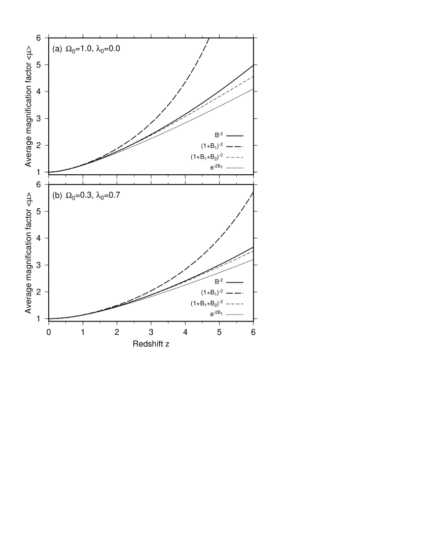
Figure 2: Average magnification factor $\left<\mu\right>$: Figure (a) shows the average magnification factor in the model of $\Omega_{0}=1.0,\lambda_{0}=0.0$. Figure (b) does in the model of $\Omega_{0}=0.3,\lambda_{0}=0.7$. The thick solid line, thick long-dashed line, dashed line and dotted line line show $B^{-2}(z)$, $(1+B_{1})^{-2}=(1-\tau)^{-2}$, $(1+B_{1}+B_{2})^{-2}$ and $e^{-2B_{1}(z)}=e^{2\tau}$, respectively.

Since our universe is locally inhomogeneous, on-average homogeneous, it is needed to know how a light ray propagate in the universe. Unfortunately we have no such cosmological model derived from the Einstein equation, then we have to investigate which working model to be plausible is reasonable and useful to discuss the problem. In this point of view, our conclusion that the gravitationally magnified angular diameter distance $\tilde{d}(0;z)$ reduces to $d_{\mathrm{FL}}(0;z)$ in the continuous limit is the important result which guarantees the fact that the hypothetical clumpy universe taken the gravitational lens effects into account is the reasonable working model to study the light ray propagation in the inhomogeneous universe.

Appendix A Background Universe Model and Angular Diameter Distance

The metric of the Friedmann–Lemaître universe (the FL universe) is given by

$$ds^{2}=c^{2}dT^{2}-a^{2}(T)\left({dr^{2}\over 1-kr^{2}}+r^{2}d\theta^{2}+r^{2}\sin^{2}\theta d\phi^{2}\right),$$ (A1)

where $T$ is the cosmological time, and $a(T)$ is the expansion factor which has the dimension of distance. The Einstein equation in this geometry yields the following relation

$$\left({\dot{a}\over a}\right)^{2}={8\pi G\over 3}\bar{\rho}(z)+{\Lambda c^{2}\over 3}-{kc^{2}\over a^{2}},$$ (A2)

where $\bar{\rho}(z)$ and $\Lambda$ are the mean density of the universe at redshift $z$ and the cosmological constant, respectively, and the dot denotes the derivative with $T$. Since $\bar{\rho}(z)$ and $a(T)$ are given in terms of their present values $\bar{\rho}_{0}$ and $a_{0}$ by $\bar{\rho}(z)=\bar{\rho}_{0}(1+z)^{3}$ and $a(T)=a_{0}/(1+z)$, respectively, equation (A2) is rewritten as

$$\left({\dot{a}\over a}\right)^{2}=H_{0}^{2}\left[\Omega_{0}(1+z)^{3}+\lambda_{0}-K(1+z)^{2}\right]\equiv H_{0}^{2}Y^{2}(z),$$ (A3)

where $\Omega_{0}=8\pi G\bar{\rho}_{0}/3H_{0}^{2}$, $\lambda_{0}=\Lambda c^{2}/3H_{0}^{2},K=kc^{2}/H_{0}^{2}a_{0}^{2}(=\Omega_{0}+\lambda_{0}-1)$ and $H_{0}$ is the present Hubble constant.

It follows from equation (A3) that the relation between $T$ and $z$ is expressed as

$$-cdT={c\over H_{0}}{dz\over(1+z)Y(z)}.$$ (A4)

Furthermore the relation between $z$ and an affine parameter $v$ along a light ray is derived from equation (A4) and from the geodesic equation for the light ray as follows:

$$dv={dz\over(1+z)^{2}Y(z)}.$$ (A5)

The dimensionless angular diameter distance $d(z_{a};z_{b})$ from a lens at redshift $z_{a}$ to another at $z_{b}$ of the clumpy universe in which a mass fraction $\bar{\alpha}$ of the mean matter density is smoothly distributed satisfies the following equation

$$(1+z_{b})^{2}Y(z_{b}){d\ \over dz_{b}}\left\{(1+z_{b})^{2}Y(z_{b}){d\ \over dz_{b}}d(z_{a};z_{b})\right\}+\frac{3}{2}\Omega_{0}\bar{\alpha}(1+z_{b})^{5}d(z_{a};z_{b})=0,$$ (A6)

and the following initial condition

$$d(z_{a};z_{b})\Bigr{|}_{z_{b}=z_{a}}=0,\qquad{d\over dz_{b}}d(z_{a};z_{b})\Bigr{|}_{z_{b}=z_{a}}={1\over(1+z_{a})Y(z_{a})},$$ (A7)

(Dyer & Roeder, 1973). The second condition is the Hubble law at redshift $z_{a}$ (Schneider et al., 1992).

Schneider et al. (1992) define the $\chi$-function in order to express a time delay function by

$$\chi_{ab}={(1+z_{a})d(0;z_{a})d(0;z_{b})\over d(z_{a};z_{b})}={1\over\chi_{a}-\chi_{b}}.$$ (A8)

The relation between the $\chi$-function and redshift $z$ is also rewritten as

$$\chi_{a}=\chi(z_{a})=\int_{z_{a}}^{\infty}{dz\over(1+z)^{2}Y(z)d^{2}(0;z)},$$ (A9)

(see also Seitz, Schneider & Ehlers, 1994).

Appendix B Proof of equation (20)

In this appendix, we prove that the equation (20) holds. In equation (21), the matrix $\tilde{U}_{i}$ is a function of $\mbox{\boldmath$\theta$}_{i}-\mbox{\boldmath$\xi$}_{i}-\tilde{\mbox{\boldmath$\theta$}}_{i}$. Then, by transforming variables $\mbox{\boldmath$\xi$}_{i}$ to $\mbox{\boldmath$\phi$}_{i}\equiv\mbox{\boldmath$\xi$}_{i}+\tilde{\mbox{\boldmath$\theta$}}_{i}-\mbox{\boldmath$\theta$}_{i}$ and putting $V_{i}(\mbox{\boldmath$\phi$}_{i})=\tilde{U}_{i}(\mbox{\boldmath$\xi$}_{i};\mbox{\boldmath$\theta$}_{i})$, we have

$$\int\!\!\!\!\int_{\cal D}d^{2}\mbox{\boldmath$\xi$}_{i_{1}}\cdots\int\!\!\!\!\int_{\cal D}d^{2}\mbox{\boldmath$\xi$}_{i_{k}}\tilde{U}_{i_{1}}(\mbox{\boldmath$\xi$}_{i_{1}};\mbox{\boldmath$\theta$}_{i_{1}})\tilde{U}_{i_{2}}(\mbox{\boldmath$\xi$}_{i_{2}};\mbox{\boldmath$\theta$}_{i_{2}})\cdots\tilde{U}_{i_{k}}(\mbox{\boldmath$\xi$}_{i_{k}};\mbox{\boldmath$\theta$}_{i_{k}})$$ (B1)

$$= \int\!\!\!\!\int_{\cal D}d^{2}\mbox{\boldmath$\phi$}_{i_{1}}\cdots\int\!\!\!\!\int_{\cal D}d^{2}\mbox{\boldmath$\phi$}_{i_{k}}\Biggl{|}{\partial(\mbox{\boldmath$\xi$}_{i_{1}}\cdots\mbox{\boldmath$\xi$}_{i_{k}})\over\partial(\mbox{\boldmath$\phi$}_{i_{1}}\cdots\mbox{\boldmath$\phi$}_{i_{k}})}\Biggr{|}V_{i_{1}}(\mbox{\boldmath$\phi$}_{i_{1}})\cdots V_{i_{k}}(\mbox{\boldmath$\phi$}_{i_{k}}),$$

where is $\partial(\mbox{\boldmath$\xi$}_{i_{1}}\cdots\mbox{\boldmath$\xi$}_{i_{k}})/\partial(\mbox{\boldmath$\phi$}_{i_{1}}\cdots\mbox{\boldmath$\phi$}_{i_{k}})$ is the Jacobian matrix. We define a $2\times 2$ sub-Jacobian matrix $J_{k}^{i}$ as

$$J_{k}^{i}={\partial\mbox{\boldmath$\phi$}_{i}\over\partial\mbox{\boldmath$\xi$}_{k}},$$

then the inverse Jacobian matrix can be written as follows:

$${\partial(\mbox{\boldmath$\phi$}_{i_{1}}\cdots\mbox{\boldmath$\phi$}_{i_{k}})\over\partial(\mbox{\boldmath$\xi$}_{i_{1}}\cdots\mbox{\boldmath$\xi$}_{i_{k}})}=\left(\begin{array}[]{ccc}J_{i_{1}}^{i_{1}}&\ldots&J_{i_{1}}^{i_{k}}\\ \vdots&\ddots&\vdots\\ J_{i_{k}}^{i_{1}}&\ldots&J_{i_{k}}^{i_{k}}\\ \end{array}\right).$$ (B2)

From equation (4) it can be shown that $\mbox{\boldmath$\theta$}_{i}$ does not depend on $\mbox{\boldmath$\xi$}_{k}$ for $k\geq i$ and then that $J_{i_{1}}^{i_{1}}=J_{i_{2}}^{i_{2}}=\cdots=J_{i_{k}}^{i_{k}}=I$ and $J_{i_{k}}^{i_{l}}=O$ for $i_{l}>i_{k}$. Thus we find the inverse Jacobian matrix has a form given by

$${\partial(\mbox{\boldmath$\phi$}_{i_{1}}\cdots\mbox{\boldmath$\phi$}_{i_{k}})\over\partial(\mbox{\boldmath$\xi$}_{i_{1}}\cdots\mbox{\boldmath$\xi$}_{i_{k}})}=\left(\begin{array}[]{cccc}I&J_{i_{1}}^{i_{2}}&\ldots&J_{i_{1}}^{i_{k}}\\ O&I&\ddots&\vdots\\ \vdots&\ddots&\ddots&J_{i_{k-1}}^{i_{k}}\\ O&\ldots&O&I\\ \end{array}\right).$$ (B3)

This matrix is a upper triangle matrix of which diagonal component is 1 and then the determinant of the matrix is unity. And therefore the determinant of the inverse matrix which is the Jacobian of mapping $\mbox{\boldmath$\xi$}_{i}\to\mbox{\boldmath$\phi$}_{i}=\mbox{\boldmath$\xi$}_{i}-\mbox{\boldmath$\theta$}_{i}-\mbox{\boldmath$\eta$}_{i}$ is unity, too. Thus the right hand side of equation (B1) can be rewritten as

$$\int\!\!\!\!\int_{\cal D}d^{2}\mbox{\boldmath$\phi$}_{i_{1}}\cdots\int\!\!\!\!\int_{\cal D}d^{2}\mbox{\boldmath$\phi$}_{i_{k}}\Biggl{|}{\partial(\mbox{\boldmath$\xi$}_{i_{1}}\cdots\mbox{\boldmath$\xi$}_{i_{k}})\over\partial(\mbox{\boldmath$\phi$}_{i_{1}}\cdots\mbox{\boldmath$\phi$}_{i_{k}})}\Biggr{|}V_{i_{1}}(\mbox{\boldmath$\phi$}_{i_{1}})\cdots V_{i_{k}}(\mbox{\boldmath$\phi$}_{i_{k}})$$

$$\hskip 56.9055pt=\left[\int\!\!\!\!\int_{\cal D}V_{i_{1}}(\mbox{\boldmath$\phi$}_{i_{1}})d^{2}\mbox{\boldmath$\phi$}_{i_{1}}\right]\cdots\left[\int\!\!\!\!\int_{\cal D}V_{i_{k}}(\mbox{\boldmath$\phi$}_{i_{k}})d^{2}\mbox{\boldmath$\phi$}_{i_{k}}\right].$$ (B4)

From (B1) and (B4) we have equation (20).