Optical spectrum of the planetary nebula M 2-24

We have obtained medium-resolution, deep optical long-slit spectra of the bulge planetary nebula (PN) M 2-24. The spectrum covers the wavelength range from 3610–7330 Å. Over two hundred emission lines have been detected. The spectra show a variety of optical recombination lines (ORLs) from C, N, O and Ne ions. The diagnostic diagram shows significant density and temperature variations across the nebula. Our analysis suggests that the nebula has a dense central emission core. The nebula was thus studied by dividing it into two regions: 1) an high ionization region characterized by an electron temperature of $T_{\rm e}=16\,300$ K and a density of $\log\,N_{\rm e}({\rm cm}^{-3})=6.3$; and 2) a low ionization region represented by $T_{\rm e}=11\,400$ K and $\log\,N_{\rm e}({\rm cm}^{-3})=3.7$. A large number of ORLs from C, N, O and Ne ions have been used to determine the abundances of these elements relative to hydrogen. In general, the resultant abundances are found to be higher than the corresponding values deduced from collisionally excited lines (CELs). This bulge PN is found to have large enhancements in two $\alpha$-elements, magnesium and neon.

1 Introduction

M 2-24 (PK 356–5° 2) is a compact (angular radius $\sim 4$ arcsec), faint [$\log F({\rm H}\beta)=-12.10$ (erg cm^-2 s^-1); Cahn et al. cahn1992 (1992)] planetary nebula in the Galactic bulge. Beaulieu et al. (beaulieu (1999)) measured its heliocentric radial velocity as 137 km s^-1. Using a statistical method, Zhang (zhang (1995)) obtained a distance of 11.79 kpc for M 2-24. Similar to IC 4997 (Hyung et al. hyung1994 (1994)), the spectrum of M 2-24 shows an extremely large [O iii] $\lambda 4363$ to H$\gamma$ $\lambda 4340$ intensity ratio, suggesting that it may have a high-density emission core. The presence of large density inhomogeneities in a nebula could lead to erroneous elemental abundances determined using the empirical method based on collisionally excited lines (CELs; Zhang & Liu zhangliu (2002)).

The determination of abundances in PNe provide very important constraints on the nuclear and mixing processes in their progenitor stars and on the chemical evolution of galaxies. Some recent chemical abundance studies of PNe in the Galactic Bulge are given by Ratag et al. ratag92 (1992), Ratag et al. ratag97 (1997), Cuisinier et al. cuisinier (2000), Escuder & Costa escuder (2001). However, in all these studies, the heavy element abundances relative to hydrogen were based on CELs only.

We have obtained medium-resolution, deep optical long-slit spectra of the bulge PN M 2-24. A large number of optical recombination lines (ORLs) detected in its spectrum can be used to determine elemental abundances. Unlike CELs, ionic abundances derived from ORLs are insensitive to the electron temperature and density in the emission region. Thus the presence of a high-density emission core in M 2-24 will hardly affect the abundances determined from ORLs. A long-standing problem in nebular abundance studies has been that the heavy-element abundance derived from ORLs are systematically higher than those derived from CELs (see Liu liua (2001, 2003) for recent reviews). As we show in this paper, even in the PNe with very dense cores, the large density fluctuation cannot completely explain the discrepancies between the ORL and CEL abundances. Based on detailed studies of several PNe, Liu (liua (2001)) concluded that the large discrepancies between the ORL and CEL abundances observed in some nebulae are mostly caused by the presence of extremely cold H-deficient inclusions embedded in normal nebular material.

In Sect. 2 of this paper, we describe our new optical observations of M 2-24 and data reduction and present the observed line fluxes. Dust extinction towards M 2-24 is discussed in Sect. 3. Plasma diagnostic analyses are presented in Sect. 4. In Sect. 5, we present and discuss the ionic and elemental abundances derived from both ORLs and CELs. A general discussion then follows in Sect. 6.

2 Observations and data reduction

Table 1: Observational journal

Date	$\lambda$-range	Slit Width	FWHM	Exp. Time
	(Å)	(arcsec)	(Å)	(sec)
1996 Jul	3530–7430	2	4.5	60, 300
1996 Jul	3530–7430	8	4.5	60
2001 Jun	3500–4805	2	1.5	900, 1800

The observations were carried out with the ESO 1.52 m telescope using the long-slit spectrograph Boller & Chivens (B&C). A journal of observations is presented in Table 1. In 1996, the detector was a UV-enhanced Loral $2048\times 2048$ $15\,\mu{\rm m}\times 15\,\mu{\rm m}$ chip, which was superseded in 2001 by a $2688\times 2688$ $15\,\mu{\rm m}\times 15\,\mu{\rm m}$ chip. The B&C spectrograph has a useful slit length of about 3.5 arcmin. In order to reduce the CCD read-out noise, in 1996 the CCD was binned by a factor of two along the slit direction, yielding a spatial sampling of 1.63 arcsec per pixel projected on the sky. A slit width of 2 arcsec was used throughout except for one short exposure for which an 8 arcsec wide slit was used so that total line fluxes from the whole nebula were recorded. The slit was oriented in the north-south direction (PA$=0^{\circ}$). The wavelength range from 3530 Å–7430 Å was observed in 1996 with an effective spectral resolution of 4.5 Å, as determined from the FWHM of the calibration lamp lines. A short exposure was taken in order to obtain intensities of the brightest emission lines, which were saturated in the spectrum of 5 min exposure time. At the same slit position an additional wavelength range was observed in 2001, covering 3500 Å–4805 Å at a resolution of 1.5 Å FWHM.

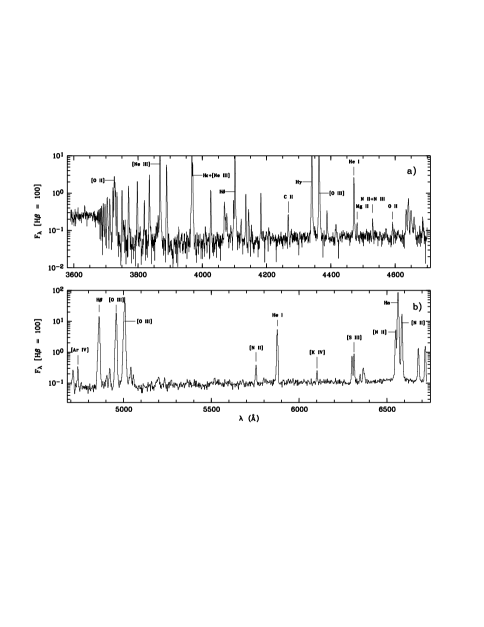
Figure 1: Optical spectrum of M 2-24 from a) 3600–4700 Å and b) 4700–6700 Å. Note that H$\alpha$ and [O iii] $\lambda$5007 were saturated in this exposure. Interstellar extinction has not been corrected for.

All the spectra were reduced using the long92 package in midas following the standard procedure. The spectra were bias-subtracted, flat-fielded and cosmic-rays removed, and then wavelength calibrated using exposures of a HeAr-CuFe calibration lamps. Absolute flux calibration was obtained by observing the standard stars Feige 110 and the nucleus of PN NGC 7293 (Walsh walsh (1993)). The extracted spectra M 2-24, after integrating along the slit, are plotted in Fig. 1. The spectra have not been corrected for interstellar extinction. The spectrum taken with an 8 arcsec wide slit yields an ${\rm H}\beta$ flux of $\log F({\rm H}\beta)=-12.11$ (erg cm^-2 s^-1), which is in good agreement with the value of -12.10 (erg cm^-2 s^-1) tabulated in Cahn et al. (cahn1992 (1992)).

All line fluxes, except those of the strongest lines, were measured using Gaussian line profile fitting. For the strongest and isolated lines, fluxes were obtained integrating over the observed line profiles. A full list of observed lines and their measured fluxes are presented in Table 2. In Table 2, column (1) gives the observed wavelengths after corrected for the Doppler shift as determined from the Balmer lines. The observed fluxes are given in column (2). Column (3) lists the fluxes after corrected for interstellar extinction, $I(\lambda)=10^{cf(\lambda)}F(\lambda)$, where $f(\lambda)$ is the standard Galactic extinction law for a total-to-selective extinction ratio of $R=3.1$ (Howarth howarth (1983)) and $c$ is the logarithmic extinction at ${\rm H}\beta$ (cf. Sect. 3). Column (4)–(10) give the ionic identification, laboratory wavelength, multiplet number, the lower and upper spectral terms of the transition, and the statistical weights of the lower and upper levels, respectively. All fluxes are normalized such that ${\rm H}\beta=100$.

Table 2: Observed relative line fluxes, on a scale where H$\beta=100$.

$\lambda_{\rm obs}$	$F(\lambda)$	$I(\lambda)$	Ion	$\lambda_{\rm lab}$	Mult	Lower Term	Upper Term	$g_{1}$	$g_{2}$
(1)	(2)	(3)	(4)	(5)	(6)	(7)	(8)	(9)	(10)
3613.19	0.266	0.443	He I	3613.64	V6	2s 1S	5p 1P*	1	3
3634.05	0.507	0.837	He I	3634.25	V28	2p 3P*	8d 3D	9	15
3673.79	0.364	0.593	H 23	3673.74	H23	2p+ 2P*	23d+ 2D	8	*
3676.47	0.502	0.818	H 22	3676.36	H22	2p+ 2P*	22d+ 2D	8	*
3679.46	0.536	0.873	H 21	3679.36	H21	2p+ 2P*	21d+ 2D	8	*
3682.92	0.603	0.981	H 20	3682.81	H20	2p+ 2P*	20d+ 2D	8	*
3686.80	0.704	1.143	H 19	3686.83	H19	2p+ 2P*	19d+ 2D	8	*
3691.77	0.872	1.413	H 18	3691.56	H18	2p+ 2P*	18d+ 2D	8	*
3697.29	0.981	1.590	H 17	3697.15	H17	2p+ 2P*	17d+ 2D	8	*
3704.28	1.900	3.067	H 16	3703.86	H16	2p+ 2P*	16d+ 2D	8	*
	*	*	He I	3705.02	V25	2p 3P*	7d 3D	9	15
3707.79	0.111	0.179	O III	3707.25	V14	3p 3P	3d 3D*	3	5
3712.13	1.520	2.449	H 15	3711.97	H15	2p+ 2P*	15d+ 2D	8	*
	*	*	O III	3715.08	V14	3p 3P	3d 3D*	5	7
3721.93	2.680	4.303	H 14	3721.94	H14	2p+ 2P*	14d+ 2D	8	*
	*	*	[S III]	3721.63	F2	3p2 3P	3p2 1S	3	1
3726.19	6.090	9.777	[O II]	3726.03	F1	2p3 4S*	2p3 2D*	4	4
3728.48	2.590	4.150	[O II]	3728.82	F1	2p3 4S*	2p3 2D*	4	6
3734.40	1.930	3.087	H 13	3734.37	H13	2p+ 2P*	13d+ 2D	8	*
3750.19	2.360	3.761	H 12	3750.15	H12	2p+ 2P*	12d+ 2D	8	*
3754.67	0.296	0.471	O III	3754.69	V2	3s 3P*	3p 3D	3	5
3756.74	0.170	0.270	O III	3757.24	V2	3s 3P*	3p 3D	1	3
3759.88	0.160	0.254	O III	3759.87	V2	3s 3P*	3p 3D	5	7
3770.69	2.890	4.572	H 11	3770.63	H11	2p+ 2P*	11d+ 2D	8	*
3774.17	0.128	0.202	O III	3774.02	V2	3s 3P*	3p 3D	3	3
3777.64	0.125	0.197	Ne II	3777.14	V1	3s 4P	3p 4P*	2	4
3790.95	0.071	0.111	O III	3791.27	V2	3s 3P*	3p 3D	5	5
3797.91	3.720	5.831	H 10	3797.90	H10	2p+ 2P*	10d+ 2D	8	*
3806.57	0.186	0.290	He I	3805.74	V63	2p 1P*	11d 1D	3	5
3814.25	0.027	0.042	He II	3813.50	4.19	4f+ 2F*	19g+ 2G	32	*
3819.69	1.090	1.696	He I	3819.62	V22	2p 3P*	6d 3D	9	15
3835.37	5.260	8.139	H 9	3835.39	H9	2p+ 2P*	9d+ 2D	8	*
3856.56	0.158	0.243	O II	3856.13	V12	3p 4D*	3d 4D	4	2
	*	*	Si II	3856.02	V1	3p2 2D	4p 2P*	6	4
3859.06	0.123	0.189	He II	3858.07	4.17	4f+ 2F*	17g+ 2G	32	*
3862.63	0.461	0.707	Si II	3862.60	V1	3p2 2D	4p 2P*	4	2
3868.63	95.900	146.494	[Ne III]	3868.75	F1	2p4 3P	2p4 1D	5	5
3882.09	0.086	0.131	O II	3882.19	V12	3p 4D*	3d 4D	8	8
	*	*	O II	3882.45	V11	3p 4D*	3d 4P	4	4
	*	*	O II	3883.13	V12	3p 4D*	3d 4D	8	6
3888.93	9.960	15.103	H 8	3889.05	H8	2p+ 2P*	8d+ 2D	8	*
	*	*	He I	3888.65	V2	2s 3S	3p 3P*	3	9
3926.64	0.157	0.235	He I	3926.54	V58	2p 1P*	8d 1D	3	5
3967.40	27.900	41.153	[Ne III]	3967.46	F1	2p4 3P	2p4 1D	3	5
3970.00	10.800	15.901	H 7	3970.07	H7	2p+ 2P*	7d+ 2D	8	98
4009.49	0.191	0.277	He I	4009.26	V55	2p 1P*	7d 1D	3	5
4026.27	2.070	2.981	He I	4026.21	V18	2p 3P*	5d 3D	9	15
	*	*	N II	4026.08	V39b	3d 3F*	4f 2[5]	7	9
4035.79	0.062	0.089	N II	4035.08	V39a	3d 3F*	4f 2[4]	5	7
4041.47	0.045	0.065	N II	4041.31	V39b	3d 3F*	4f 2[5]	9	11
4045.82	0.087	0.124	[Fe III]	4046.40		3d6 5D	3d6 3G	7	7
4048.12	0.038:	0.054	O II	4048.21	V50b	3d 4F	4f F3*	8	8
4062.83	0.037:	0.052	O II	4062.94	V50a	3d 4F	4f F4*	10	10
4069.06	1.340	1.898	[S II]	4068.60	F1	2p3 4S*	2p3 2P*	4	4
4072.02	0.200	0.283	O II	4071.23	V48a	3d 4F	4f G5*	8	10
	*	*	O II	4072.16	V10	3p 4D*	3d 4F	6	8
4076.30	0.555	0.783	[S II]	4076.35	F1	2p3 4S*	2p3 2P*	2	4
4079.34	0.050:	0.071	O II	4078.84	V10	3p 4D*	3d 4F	4	4
4088.89	0.196	0.275	O II	4089.29	V48a	3d 4F	4f G5*	10	12
4097.42	1.140	1.597	N III	4097.33	V1	3s 2S	3p 2P*	2	4
	*	*	O II	4097.25	V20	3p 4P*	3d 4D	2	4
	*	*	O II	4097.26	V48b	3d 4F	4f G4*	8	10

Table 2: –continued

$\lambda_{\rm obs}$	$F(\lambda)$	$I(\lambda)$	Ion	$\lambda_{\rm lab}$	Mult	Lower Term	Upper Term	$g_{1}$	$g_{2}$
(1)	(2)	(3)	(4)	(5)	(6)	(7)	(8)	(9)	(10)
	*	*	O II	4098.24	V46a	3d 4F	4f D3*	4	6
4101.81	19.600	27.407	H 6	4101.74	H6	2p+ 2P*	6d+ 2D	8	72
4120.80	0.466	0.647	O II	4119.22	V20	3p 4P*	3d 4D	6	8
	*	*	O II	4120.28	V20	3p 4P*	3d 4D	6	6
	*	*	O II	4120.54	V20	3p 4P*	3d 4D	6	4
	*	*	He I	4120.84	V16	2p 3P*	5s 3S	9	3
	*	*	O II	4121.46	V19	3p 4P*	3d 4P	2	2
4144.16	0.699	0.960	He I	4143.76	V53	2p 1P*	6d 1D	3	5
4152.64	0.167	0.228	O II	4153.30	V19	3p 4P*	3d 4P	4	6
4156.61	0.075	0.102	O II	4156.53	V19	3p 4P*	3d 4P	6	4
4186.27	0.120	0.162	C III	4186.90	V18	4f 1F*	5g 1G	7	9
4190.54	0.087	0.117	O II	4189.79	V36	3p′ 2F*	3d′ 2G	8	10
4199.85	0.213	0.286	He II	4199.83	4.11	4f+ 2F*	11g+ 2G	32	*
	*	*	N III	4200.10	V6	3s′ 2P*	3p′ 2D	4	6
4206.63	0.141	0.189	[Fe IV]	4206.60		3d5 4G	3d5 2H	10	10
4209.31	0.120	0.161	[Fe IV]	4208.90		3d5 4G	3d5 2H	8	10
4228.01	0.040:	0.053	N II	4227.74	V33	3p 1D	4s 1P*	5	3
	*	*	[Fe V]	4227.20	F2	3d4 5D	3d4 3H	9	9
4237.08	0.046	0.060	N II	4236.91	V48a	3d 3D*	4f 1[3]	3	5
	*	*	N II	4237.05	V48b	3d 3D*	4f 1[4]	5	7
4258.64	0.054	0.071	[Fe III]	4257.20		3d6 3P	3d6 1F	5	7
4267.46	0.504	0.657	C II	4267.15	V6	3d 2D	4f 2F*	10	14
4274.46	0.046	0.059	O II	4273.10	V67a	3d 4D	4f F4*	6	8
4275.85	0.029:	0.038	O II	4275.55	V67a	3d 4D	4f F4*	8	10
	*	*	O II	4275.99	V67b	3d 4D	4f F3*	4	6
	*	*	O II	4276.28	V67b	3d 4D	4f F3*	6	6
	*	*	O II	4276.75	V67b	3d 4D	4f F3*	6	8
4277.56	0.126	0.164	O II	4277.43	V67c	3d 4D	4f F2*	2	4
	*	*	O II	4277.89	V67b	3d 4D	4f F3*	8	8
4280.61	0.035	0.046	O II	4281.32	V53b	3d 4P	4f D2*	6	6
4283.10	0.021	0.028	O II	4282.96	V67c	3d 4D	4f F2*	4	6
4284.67	0.038	0.050	O II	4283.73	V67c	3d 4D	4f F2*	4	4
4286.85	0.079	0.102	O II	4285.69	V78b	3d 2F	4f F3*	6	8
4289.54	0.063	0.081	O II	4288.82	V53c	3d 4P	4f D1*	2	4
	*	*	O II	4288.82	V53c	3d 4P	4f D1*	2	2
4292.26	0.029	0.038	C II	4292.16		4f 2F*	10g 2G	14	18
	*	*	O II	4292.21	V78c	3d 2F	4f F2*	6	6
4317.45	0.071	0.091	O II	4317.14	V2	3s 4P	3p 4P*	2	4
	*	*	O II	4317.70	V53a	3d 4P	4f D3*	4	6
4319.74	0.042	0.054	O II	4319.63	V2	3s 4P	3p 4P*	4	6
4333.12	0.092	0.117	O II	4332.71	V65b	3d 4D	4f G4*	8	10
4340.56	39.200	49.532	H 5	4340.47	H5	2p+ 2P*	5d+ 2D	8	50
4350.07	0.220	0.277	O II	4349.43	V2	3s 4P	3p 4P*	6	6
4352.94	0.074	0.093	O II	4353.59	V76c	3d 2F	4f G3*	6	8
4363.21	56.000	69.982	[O III]	4363.21	F2	2p2 1D	2p2 1S	5	1
4369.31	0.052	0.065	Ne II	4369.86	V56	3d 4F	4f 0[3]*	4	6
4378.91	0.098	0.121	N III	4379.11	V18	4f 2F*	5g 2G	14	18
	*	*	Ne II	4379.55	V60b	3d 3F	4f 1[4]*	8	10
4388.24	0.628	0.776	He I	4387.93	V51	2p 1P*	5d 1D	3	5
4391.41	0.048	0.059	Ne II	4391.99	V55e	3d 4F	4f 2[5]*	10	12
	*	*	Ne II	4392.00	V55e	3d 4F	4f 2[5]*	10	10
4413.12	0.074	0.091	Ne II	4413.22	V65	3d 4P	4f 0[3]*	6	8
	*	*	Ne II	4413.11	V57c	3d 4F	4f 1[3]*	4	6
	*	*	Ne II	4413.11	V65	3d 4P	4f 0[3]*	6	6
4415.60	0.109	0.133	O II	4414.90	V5	3s 2P	3p 2D*	4	6
4418.05	0.180	0.220	O II	4416.97	V5	3s 2P	3p 2D*	2	4
4428.13	0.071	0.087	Ne II	4428.64	V60c	3d 2F	4f 1[3]*	6	8
	*	*	Ne II	4428.52	V61b	3d 2D	4f 2[3]*	6	8
4432.97	0.028	0.034	N II	4432.74	V55a	3d 3P*	4f 2[3]	5	7
	*	*	N II	4433.48	V55b	3d 3P*	4f 2[2]	1	3
4438.15	0.109:	0.132	He I	4437.55	V50	2p 1P*	5s 1S	3	1
4471.69	5.780	6.885	He I	4471.50	V14	2p 3P*	4d 3D	9	15

Table 2: –continued

$\lambda_{\rm obs}$	$F(\lambda)$	$I(\lambda)$	Ion	$\lambda_{\rm lab}$	Mult	Lower Term	Upper Term	$g_{1}$	$g_{2}$
(1)	(2)	(3)	(4)	(5)	(6)	(7)	(8)	(9)	(10)
4481.77	0.291	0.345	Mg II	4481.21	V4	3d 2D	4f 2F*	10	14
4491.82	0.070	0.083	C II	4491.07		4f 2F*	9g 2G	14	18
	*	*	O II	4491.23	V86a	3d 2P	4f D3*	4	6
4511.03	0.156	0.183	N III	4510.91	V3	3s′ 4P*	3p′ 4D	4	6
	*	*	N III	4510.91	V3	3s′ 4P*	3p′ 4D	2	4
4514.75	0.041	0.048	N III	4514.86	V3	3s′ 4P*	3p′ 4D	6	8
4517.53	0.077	0.090	N III	4518.15	V3	3s′ 4P*	3p′ 4D	2	2
4523.33	0.080	0.093	N III	4523.58	V3	3s′ 4P*	3p′ 4D	4	4
4530.00	0.363	0.421	N II	4530.41	V58b	3d 1F*	4f 2[5]	7	9
	*	*	N III	4530.86	V3	3s′ 4P*	3p′ 4D	4	2
4592.20	0.273	0.308	O II	4590.97	V15	3s′ 2D	3p′ 2F*	6	8
4596.65	0.148	0.167	O II	4596.18	V15	3s′ 2D	3p′ 2F*	4	6
4607.29	0.072	0.081	N II	4607.16	V5	3s 3P*	3p 3P	1	3
4609.88	0.113	0.127	O II	4609.44	V92a	3d 2D	4f F4*	6	8
	*	*	O II	4610.20	V92c	3d 2D	4f F2*	4	6
4634.53	0.871	0.966	N III	4634.14	V2	3p 2P*	3d 2D	2	4
4641.25	2.020	2.231	N III	4640.64	V2	3p 2P*	3d 2D	4	6
	*	*	O II	4641.81	V1	3s 4P	3p 4D*	4	6
	*	*	N III	4641.84	V2	3p 2P*	3d 2D	4	4
4649.71	1.300	1.431	O II	4649.13	V1	3s 4P	3p 4D*	6	8
	*	*	C III	4650.25	V1	3s 3S	3p 3P*	3	3
	*	*	O II	4650.84	V1	3s 4P	3p 4D*	2	2
	*	*	C III	4651.47	V1	3s 3S	3p 3P*	3	1
4659.10	0.372	0.408	[Fe III]	4658.10	F3	3d6 5D	3d6 3F2	9	9
	*	*	C IV	4657.15		5f 2F*	6g 2G	14	18
4662.24	0.094	0.102	O II	4661.63	V1	3s 4P	3p 4D*	4	4
4676.54	0.161	0.175	O II	4676.24	V1	3s 4P	3p 4D*	6	6
4677.79	0.050	0.054	N II	4678.14	V61b	3d 1P*	4f 2[2]	3	5
4686.37	0.516	0.559	He II	4685.68	3.4	3d+ 2D	4f+ 2F*	18	32
4701.65	0.099	0.107	[Fe III]	4701.62	F3	3d6 5D	3d6 3F2	7	7
4713.46	1.240	1.327	[Ar IV]	4711.37	F1	3p3 4S*	3p3 2D*	4	6
	*	*	He I	4713.17	V12	2p 3P*	4s 3S	9	3
4733.90	0.046	0.049	[Fe III]	4733.87		3d6 5D	3d6 3F	5	5
4740.55	1.380	1.458	[Ar IV]	4740.17	F1	3p3 4S*	3p3 2D*	4	4
4860.96	100.000	100.000	H 4	4861.33	H4	2p+ 2P*	4d+ 2D	8	32
4881.98	0.216	0.214	[Fe III]	4881.11	F2	3d6 5D	3d6 3H	9	9
4904.52	0.810	0.800	O II	4906.83	V28	3p 4S*	3d 4P	4	4
	*	*	[Fe II]	4905.34		3d7 4F	4s 4F	8	8
	*	*	[Fe IV]	4906.60		3d5 4G	3d5 4F	12	10
4921.58	1.650	1.605	He I	4921.93	V48	2p 1P*	4d 1D	3	5
4958.55	128.000	122.464	[O III]	4958.91	F1	2p2 3P	2p2 1D	3	5
5006.51	394.000	368.720	[O III]	5006.84	F1	2p2 3P	2p2 1D	5	5
5032.60	0.519	0.480	[Fe IV]	5032.40		3d5 4G	3d5 2F	6	6
5041.48	1.780	1.641	Si II	5041.03	V5	4p 2P*	4d 2D	2	4
5056.10	0.657	0.601	Si II	5055.98	V5	4p 2P*	4d 2D	4	6
	*	*	Si II	5056.31	V5	4p 2P*	4d 2D	4	4
5191.28	0.226:	0.195	[Ar III]	5191.82	F3	2p4 1D	2p4 1S	5	1
5199.63	0.580	0.498	[N I]	5199.84	F1	2p3 4S*	2p3 2D*	4	4
	*	*	[N I]	5200.26	F1	2p3 4S*	2p3 2D*	4	6
5341.69	0.095	0.077	C II	5342.38		4f 2F*	7g 2G	14	18
5679.07	0.304	0.217	N II	5679.56	V3	3s 3P*	3p 3D	5	7
5754.46	1.820	1.271	[N II]	5754.60	F3	2p2 1D	2p2 1S	5	1
5798.93	0.379	0.261	C IV	5801.51	V1	3s 2S	3p 2P*	2	4
5810.84	0.296	0.203	C IV	5812.14	V1	3s 2S	3p 2P*	2	2
5875.63	30.700	20.660	He I	5875.66	V11	2p 3P*	3d 3D	9	15
5939.31	0.215	0.142	N II	5940.24	V28	3p 3P	3d 3D*	3	3
	*	*	N II	5941.65	V28	3p 3P	3d 3D*	5	7
6101.74	0.859	0.541	[K IV]	6101.83	F1	3p4 3P	3d4 1D	5	5
6301.51	3.860	2.296	[O I]	6300.34	F1	2p4 3P	2p4 1D	5	5
6312.30	4.320	2.565	[S III]	6312.10	F3	2p2 1D	2p2 1S	5	1
6347.27	0.470	0.276	Si II	6347.10	V2	4s 2S	4p 2P*	2	4
6364.79	1.250	0.731	[O I]	6363.78	F1	2p4 3P	2p4 1D	3	5

Table 2: –continued

$\lambda_{\rm obs}$	$F(\lambda)$	$I(\lambda)$	Ion	$\lambda_{\rm lab}$	Mult	Lower Term	Upper Term	$g_{1}$	$g_{2}$
(1)	(2)	(3)	(4)	(5)	(6)	(7)	(8)	(9)	(10)
6371.94	0.631	0.368	Si II	6371.38	V2	4s 2S	4p 2P*	2	2
6549.53	35.700	19.873	[N II]	6548.10	F1	2p2 3P	2p2 1D	3	5
6562.78	616.000	341.649	H 3	6562.77	H3	2p+ 2P*	3d+ 2D	8	18
6584.85	109.000	60.121	[N II]	6583.50	F1	2p2 3P	2p2 1D	5	5
6678.55	8.300	4.470	He I	6678.16	V46	2p 1P*	3d 1D	3	5
6718.03	9.840	5.241	[S II]	6716.44	F2	2p3 4S*	2p3 2D*	4	6
6732.54	13.000	6.898	[S II]	6730.82	F2	2p3 4S*	2p3 2D*	4	4
7064.86	18.500	9.069	He I	7065.25	V10	2p 3P*	3s 3S	9	3
7136.23	13.400	6.461	[Ar III]	7135.80	F1	3p4 3P	3p4 1D	5	5
7159.25	0.725	0.348	He I	7160.56		3s 3S	10p 3P*	3	9
7169.69	1.410	0.674	[Ar IV]	7170.62	F2	3p3 2D*	3p3 2P*	4	4
7236.13	1.370	0.646	C II	7236.42	V3	3p 2P*	3d 2D	4	6
	*	*	C II	7237.17	V3	3p 2P*	3d 2D	4	4
	*	*	[Ar IV]	7237.26	F2	3p3 2D*	3p3 2P*	6	4
7262.24	0.991	0.464	[Ar IV]	7262.76	F2	3p3 2D*	3p3 2P*	4	2
7280.34	1.430	0.667	He I	7281.35	V45	2p 1P*	3s 1S	3	1
7296.07	0.454:	0.211	He I	7298.04		3s 3S	9p 3P*	3	9
7320.07	1.800	0.833	[O II]	7318.92	F2	2p3 2D*	2p3 2P*	6	2
	*	*	[O II]	7319.99	F2	2p3 2D*	2p3 2P*	6	4
7330.40	2.240	1.033	[O II]	7329.67	F2	2p3 2D*	2p3 2P*	4	2
	*	*	[O II]	7330.73	F2	2p3 2D*	2p3 2P*	4	4

3 Reddening summary

Table 3: Extinction derived from the Balmer decrement

Balmer decrement	Ratio	$c({\rm H}\beta)$
H$\alpha$/H$\beta$	6.16	1.08
H$\gamma$/H$\beta$	0.39	0.65
H$\delta$/H$\beta$	0.20	0.70
Adopted		0.80

The measured H$\alpha$/H$\beta$, H$\gamma$/H$\beta$, and H$\delta$/H$\beta$ ratios, together with the logarithmic extinction at H$\beta$, $c=\log I({\rm H}\beta)/F({\rm H}\beta)$, derived from these ratios using the Galactic reddening law of Howarth (howarth (1983)), are listed in Table 3. The extinction derived from the H$\alpha$/H$\beta$ ratio is higher than those derived from the higher order Balmer lines, suggesting possible self-absorption effects caused by significant optical depths in the Balmer lines. The Balmer line ratios H$\alpha$/H$\beta$ and H$\gamma$/H$\beta$ as a function of the optical depths of Ly $\alpha$ and H $\alpha$ are given by Cox & Mathews (cox (1969)). For an H $\alpha$ optical depth of 5, the observed H$\alpha$/H$\beta$ and H$\gamma$/H$\beta$ ratios yield very similar reddening constants of $c({\rm H}\beta)=0.80$. For comparison, the observed total H$\beta$ flux, $\log F({\rm H}\beta)=-12.11$ erg cm^-2 s^-1 and the 5-GHz radio free-free continuum flux density, $S(5\,{\rm GHz})=0.003$ Jy, for M 2-24 (Cahn et al. cahn1992 (1992)) yield a very low value, $c({\rm H}\beta)=0.08$. It is possible that the radio flux density for this faint PN may have been significantly underestimated, leading to an underestimated interstellar extinction constant. On the other hand, it is also possible, as has been known for some time (Stasíska et al. stasinska (1992); Walton, Barlow & Clegg walton (1993); Liu et al. liu2001 (2001)), the standard interstellar extinction law ($R_{V}=3.1$) may not be applicable to the lines-of-sight towards Galactic bulge PNe. Here we have adopted $c({\rm H}\beta)=0.80$, as derived from the observed Balmer line ratios after corrected for the optical depth effects, to deredden the optical spectra.

4 Plasma diagnostics

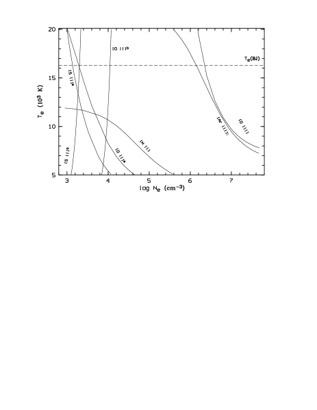
Figure 2: Plasma diagnostic diagram for M 2-24. The dashed line shows the hydrogen Balmer jump temperature.

In the optical spectrum of M 2-24, a number of CELs, which are useful for nebular diagnostic analysis and abundance determinations, are observed. The electron temperatures and densities derived from various CEL diagnostic ratios were obtained by solving the level populations for multilevel ($\geq 5$) atomic models. The plasma diagnostic diagram based on these line ratios are plotted in Fig. 2. The ratios employed were [N ii] $(\lambda 6548+\lambda 6584)/\lambda 5754$, [O ii]^a $(\lambda 7320+\lambda 7330)/(\lambda 3726+\lambda 3729)$, [O ii]^b $\lambda 3726/\lambda 3729$, [S ii]^a $(\lambda 4068+\lambda 4076)/(\lambda 6731+\lambda 6716)$, [S ii]^b $\lambda 6731/\lambda 6716$, [O iii] $(\lambda 4959+\lambda 5007)/\lambda 4363$ and [Ar iii] $\lambda 7135/\lambda 5192$. Note that the intensity of the weak line [Ar iii] $\lambda 5192$ has a relatively large uncertainty making the [Ar iii] $\lambda 7135/\lambda 5192$ ratio less reliable as a plasma diagnostic. According to the intersectant points of the temperature diagnostic [N ii] $(\lambda 6548+\lambda 6584)/\lambda 5754$ with four density diagnostics [O ii]^a $(\lambda 7320+\lambda 7330)/(\lambda 3726+\lambda 3729)$, [O ii]^b $\lambda 3726/\lambda 3729$, [S ii]^a $(\lambda 4068+\lambda 4076)/(\lambda 6731+\lambda 6716)$ and [S ii]^b $\lambda 6731/\lambda 6716$, we can conclude that the singly ionized regions can be characterized by a temperature of $T_{\rm e}=11\,400\pm 500$ K and a density of $\log N_{\rm e}({\rm cm}^{-3})=3.7\pm 0.4$. On the other hand, emission from doubly ionized species such as [O iii] $(\lambda 4959+\lambda 5007)/\lambda 4363$ appear to arise from a separate high density emission region.

Table 4: Plasma diagnostics

Ion	Lines	Ionization Potential (eV)	Ratio	Result
				$\log N_{\rm e}$ (cm-3)
[S ii]	$I(\lambda 6731)/I(\lambda 6716)$	10.36	1.32	3.25a
[S ii]	$I(\lambda 4068+\lambda 4076)/I(\lambda 6731+\lambda 6716)$	10.36	0.22	3.38a
[O ii]	$I(\lambda 3726)/I(\lambda 3729)$	13.62	2.36	3.99a
[O ii]	$I(\lambda 7320+\lambda 7330)/I(\lambda 3726+\lambda 3729)$	13.62	0.13	3.67a
[Ar iii]	$I(\lambda 7135)/I(\lambda 5192^{\mathrm{b}})$	27.63	33.2	6.15c
[O iii]	$I(\lambda 4959+\lambda 5007)/I(\lambda 4363)$	35.12	6.56	6.35c
Balmer decrement				6–7
				$T_{\rm e}$ (K)
[N ii]	$I(\lambda 6548+\lambda 6584)/I(\lambda 5754)$	14.53	59.55	11400d
BJ/H 11				16300

• Assuming $T_{\rm e}=11\,400$ K;

• Poor quality;

• Assuming $T_{\rm e}=16\,300$ K;

• Assuming $\log N_{\rm e}({\rm cm}^{-3})=3.7$.

Fig. 2 also shows the Balmer jump (BJ) temperature derived from the ratio of the nebular continuum Balmer discontinuity at 3646 Å to H 11 $\lambda 3770$ (Fig. 3), using the formula given by Liu et al. (liu2001 (2001)). We used the ratio of the Balmer discontinuity to H 11 rather than to H$\beta$, since the temperature thus derived is much less sensitive to uncertainties in the reddening correction and flux calibration, given the small wavelength difference between the Balmer discontinuities and H 11. The He⁺/H⁺ and He⁺⁺/H⁺ ionic abundance ratios, which are needed to calculate $T_{\rm e}$(BJ), are taken from Sect. 5. We found $T_{\rm e}(\rm{BJ})=16\,300$ K, which is about 5000 K higher than the temperature implied by the nebular diagnostics from singly ionized species.

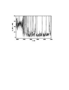
Figure 3: Spectrum of M 2-24 from 3580–4100 Å, showing the nebular continuum Balmer discontinuity at 3646 Å. The dashed line is an empirical fit to the continuum level. The spectrum has not been corrected for extinction and is normalized such that $F({\rm H\beta})=100$.

If we assume that the [O iii] and [Ar iii] lines arise from a hotter region of $T_{\rm e}(\rm{BJ})=16\,300$ K, then the [O iii] and [Ar iii] diagnostic ratios plotted in Fig. 2 would yield an electron density of $\log N_{\rm e}({\rm cm}^{-3})=6.35$ and 6.15, respectively. This would suggest that this hotter, high ionization region (dominated by doubly ionized species) is probably also much denser than the cooler region from which lines from singly ionized species arise.

That M 2-24 contains a dense emission region is supported by our analysis of its hydrogen recombination line spectrum. In Fig. 4, we plot the observed intensities of high-order hydrogen Balmer lines ($n\rightarrow 2$, $n=11,13,...,23$) as a function of the principal quantum number $n$ of the upper level. Theoretical intensities for different electron densities are also plotted assuming an electron temperature of 16 300 K, as deduced from the ratio of nebular continuum Balmer discontinuity to H 11. The intensities of the Balmer decrement are density-sensitive but depend only weakly on temperature, thus provide a valuable density diagnostic. In particular, they can be used to probe high-density ionization regions where collisionally excited diagnostic lines of relatively low critical densities are suppressed by collisional de-excitation. Given our spectral resolution, the Balmer lines can be resolved (and thus the Balmer decrement can be measured) up to $n=23$. Fig. 4 shows that the measured intensities of almost all the Balmer lines from $n=11$ to 23 yield an best fit density between $10^{6}$–$10^{7}$ cm^-3, except for H 14 $\lambda$3721.94, H 15 $\lambda$3711.97 and H 16 $\lambda$3703.86, which are blended with the [S iii] $\lambda 3721.63$, O iii $\lambda 3715.08$ and He i $\lambda 3705.12$ lines, respectively.

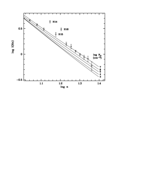
Figure 4: Observed intensities (in units where ${\rm H}\beta=100$) of the high-order Balmer lines ($n\rightarrow 2$, $n=11,13,...,23$) as a function of the principal quantum number $n$. Note H 14, H 15 and H 16 are affected by line blending. The solid lines show predicted intensities for electron densities from $N_{\rm e}=10^{3}$ to 10⁷ cm^-3, assuming an electron temperature of 16 300 K.

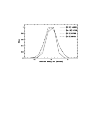
Figure 5: Spatial distribution of emission along the slit for [O iii] $\lambda 4363$, [Ar iii] $\lambda 7135$, [O ii] $\lambda 3729$ and [S ii] $\lambda 6731$ lines. For all the emission lines, the peak-values of the observed fluxes are normalized to one.

Table 4 summarizes these electron temperatures and densities derived from the various diagnostics, which suggests that [O iii] and [Ar iii] emission lines arise probably from a different region with those singly ionized species. In Fig. 5, we compare the surface brightness distributions of several emission lines along the slit. The figure shows that the spatial distribution of [O iii] $\lambda 4363$ line is similar to that of the [Ar iii] $\lambda 7135$ line, while emissions from singly ionic species such as the [O ii] $\lambda 3729$ and [S ii] $\lambda 6731$ lines are apparently from more extensive regions.

The above analysis reveals that M 2-24 has two distinct emission regions of very different physical conditions. The hotter and denser region, characterized by $T_{\rm e}=16\,300$ K and $\log N_{\rm e}({\rm cm}^{-3})=6.3$, is from a dense core close to the central star. The cooler, lower density region, characterized by $T_{\rm e}=11\,400$ K and $\log N_{\rm e}({\rm cm}^{-3})=3.7$ and dominated by emission from singly ionized species, is from an outer shell. Thus M 2-24 bears many resemblances to Mz 3 previously analyzed by us (Zhang & Liu zhangliu (2002)).

Fig. 6 illustrates $N_{\rm e}$ derived from various diagnostics as a function of Ionization Potential (IP) of the diagnostic lines. For the purpose of ionic abundance determinations (see below), we have thus divided the nebula into two regions based on IP, as indicated by the dashed line in Fig. 6.

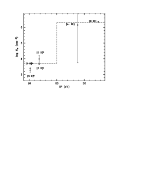
Figure 6: Electron density versus ionization potential. The dashed line shows the electron densities adopted to determine the relative ionic abundances.

5 Abundance analysis

In this section we present the elemental abundances derived from observed line intensities relative to H$\beta$. For both CELs and ORLs abundance calculations, the effective recombination coefficient of H$\beta$ was taken from Storey & Hummer (storey1995 (1995)). Based on the plasma diagnostic results, a constant temperature of $T_{\rm e}=16\,300$ K and a density of $\log N_{\rm e}({\rm cm}^{-3})=6.3$ have been assumed for ions with IP higher than 20 eV. For ions of lower IP, a constant temperature of $T_{\rm e}=11\,400$ K and a density of $\log N_{\rm e}({\rm cm}^{-3})=3.7$ have been assumed.

In Sect. 3, we showed that the Balmer line emission from the nebula is probably optically thick and estimated an optical depth of 5 for H$\alpha$. The effect of self-absorption on H$\beta$ flux has to be corrected for before the observed line intensities tabulated in Table 2 can be used to calculate the ionic abundances. The escape probability of H$\beta$ as a function of H$\alpha$ optical depth has been calculated by Cox & Mathews (cox (1969)). By interpolating their results, we derived an escape probability of 0.67 for H$\beta$ for an H$\alpha$ optical depth of 5. Consequently, we have divided all the line intensities relative to H$\beta$ tabulated in Table 2 by a factor of 0.67 before calculating the ionic abundances.

5.1 Ionic abundances from CELs

The ionic abundances are derived by

$$\frac{N({\rm X}^{i+})}{N({\rm H}^{+})}=\frac{I_{jk}}{I_{{\rm H}\beta}}\frac{\lambda_{jk}}{\lambda_{{\rm H}\beta}}\frac{\alpha_{{\rm H}\beta}}{A_{jk}}({\frac{N_{j}}{N({\rm X}^{i+})}})^{-1}N_{\rm e}$$ (1)

where $I_{jk}/I_{{\rm H}\beta}$ is the ratio of the intensity of the ionic line to H$\beta$; $\lambda_{jk}/\lambda_{{\rm H}\beta}$ is the ratio of the wavelength of the ionic line to that of H$\beta$; $\alpha_{{\rm H}\beta}$ is the effective recombination coefficient of ${\rm H}\beta$; $A_{jk}$ is the Einstein spontaneous transition probability of the ionic line; and $N_{j}/N({\rm X}^{i+}$) is the ratio of the fractional population of the upper level from which the ionic line originates, which is sensitive to the electron temperature and density. References for the adopted collision strengths and transition probabilities are listed in Table 5.

Table 5: Reference for atomic data of CELs.

Ion	IP (eV)		Reference
Xi	Xi-1	Xi	Trans. Prob.	Coll. Str.
N+	14.53	29.60	[1]	[2]
O+	13.62	35.12	[3]	[4]
O2+	35.12	54.94	[5]	[6]
Ne2+	40.90	63.45	[7]	[8]
S+	10.36	23.34	[9], [10]	[11]
S2+	23.34	34.79	[12]	[7]
Ar2+	27.63	40.74	[13]	[14]
Ar3+	40.74	59.81	[9]	[15]
Fe2+	16.19	30.65	[16]	[17]
Fe3+	30.65	54.80	[18]	[19]

• [1] Nussbaumer & Rusca (nussbaumer (1979)); [2] Stafford et al. (stafford (1994)); [3] Zeippen (zeippen1982 (1982)); [4]Pradhan (pradhan (1976)); [5] Nussbaumer & Storey (nussbaumer1981 (1981)); [6] Aggarwal (aggarwal (1983)); [7] Mendoza (mendoza1983 (1983)); [8] Butler & Zeippen (butler1994 (1994)); [9] Mendoza & Zeippen (1982a ); [10] Keenan et al. (keenan1993 (1993)); [11] Keenan et al. (keenan1996 (1996)); [12] Mendoza & Zeippen (1982b ); [13] Mendoza & Zeippen (mendozazeippen1983 (1983)); [14] Johnson & Kingston (johnson1990 (1990)); [15] Zeippen et al. (zeippen1987 (1987)); [16] Nahar & Pradhan(nahar (1996)); [17] Zhang (zhang1996 (1996)); [18] Zhang & Pradhan (zhang1997 (1996)); [19] Garstang (garstang1958 (1958)).

The ionic abundances derived from optical CELs are presented in Table 6. Given that ionic abundances derived from CELs are very sensitive to the adopted electron temperature and density, and the fact that their values in the dense central emission core of M 2-24 are not well constrained by our current observations, the results presented in Table 6 may suffer large uncertainties. Additional errors may also be introduced by the fact that not all the observed fluxes of lines with IP $>$ 20 eV arise entirely within the dense core. Conversely, not all the observed fluxes of lines with IP $<$ 20 eV arise exclusively in the the outer, less dense nebular layers. In other words, our simple two-zone model may not be sufficient for such a complicated object.

For comparison, Table 6 also gives the N⁺/H⁺, O⁺/H⁺ and S⁺/H⁺ abundance ratios derived from the [N ii] $\lambda$5754, [O ii] $\lambda\lambda$7320, 7330 and [S ii] $\lambda\lambda$4068, 4076 auroral or transauroral lines, which, owning to their higher critical densities, are less density-dependent than the [N ii] $\lambda\lambda$6548, 6584, [O ii] $\lambda\lambda$3726, 3729 and [S ii] $\lambda\lambda$6716, 6731 nebular lines. On the other hand, given their higher excitation energies, the ionic abundances derived from auroral or transauroral lines are more sensitive to the adopted $T_{\rm e}$ than those derived from nebular lines. The abundances derived from the auroral or transauroral lines are in good agreement with those deduced from the nebular lines, suggesting the adopted electron temperature and density for the low ionization region are reasonable.

Table 6: Ionic abundances of heavy elements derived from CELs.

Ion	Lines	$N_{{\rm X}^{i+}}/N_{{\rm H}^{+}}$
N+	[N ii] $\lambda\lambda$6548, 6584	5.25(-6)
	[N ii] $\lambda\lambda$5754	4.86(-6)
O+	[O ii] $\lambda\lambda$3726, 3729	3.61(-6)
	[O ii] $\lambda\lambda$7320, 7330	4.82(-6)
O2+	[O iii] $\lambda\lambda$4959, 5007	8.04(-5)
Ne2+	[Ne iii] $\lambda 3868$	2.24(-5)
S+	[S ii] $\lambda\lambda$6716, 6731	2.57(-7)
	[S ii] $\lambda\lambda$4068, 4076	1.63(-7)
S2+	[S iii] $\lambda 6312$	4.08(-7)
Ar2+	[Ar iii] $\lambda 7135$	1.93(-7)
Ar3+	[Ar iv] $\lambda 4733$	2.46(-7)
Fe2+	[Fe iii] $\lambda\lambda$4658, 4734	8.71(-8)
Fe3+	[Fe iv] $\lambda$5032	1.10(-6)

5.2 Ionic abundances from ORLs

In order to compare with the ionic abundances derived from CELs, we also determine ionic abundances using ORLs. From the measured intensities of ORLs, ionic abundances can be derived using

$$\frac{N({\rm X}^{i+})}{N({\rm H}^{+})}=\frac{I_{jk}}{I_{{\rm H}\beta}}\frac{\lambda_{jk}}{\lambda_{{\rm H}\beta}}\frac{\alpha_{{\rm H}\beta}}{\alpha_{jk}}$$ (2)

where $\alpha_{jk}$ is the effective recombination coefficient for the ionic ORL. Ionic abundances derived from ORLs depend only weakly on the adopted temperature, $\sim T_{\rm e}^{\alpha}$, where $|\alpha|\la 1$, and are essentially independent of $N_{\rm e}$ under the low density conditions (N${}_{e}\la 10^{8}$ cm^-3). As a consequence, the presence of temperature and density fluctuations will have little effects on ORL abundances. The ionic abundances derived from ORLs are presented in Table 7. ORLs blended with strong lines have large uncertainties in the measured intensities and therefore have been excluded from the table.

Table 7: Ionic abundances of M 2-24 from ORLs.

Ion	$\lambda$ (Å)	Mult	$I$	$N_{{\rm X}^{i+}}/N_{{\rm H}^{+}}$
He+	4471.50	V14	6.885	6.74(-2)
	5875.66	V11	20.66	6.41(-2)
	6678.16	V46	4.470	7.00(-2)
	Average			6.59(-2)
He2+	4685.68	3.4	0.559	3.46(-4)
C2+	4267.15	V6	0.657	4.42(-4)
C3+	4186.90	V18	0.162	1.29(-4)
N2+	5679.56	V3	0.217	2.56(-4)
	4607.16a	V5	0.080	7.32(-4)
	5940.24,1.65	V28	0.142	3.49(-4)
	4035.08	V39a	0.089	3.16(-4)
	4041.31	V39b	0.065	1.95(-4)
	4236.91,7.91	V48	0.060	1.77(-4)
	4432.74,3.48	V55	0.034	1.84(-4)
	4678.14	V61b	0.054	2.66(-4)
	Average			3.00(-4)
N3+	4379.11b	V60b	0.121	3.73(-5)
O2+	4676.24	V1	0.175	9.42(-4)
	4661.63	V1	0.102	4.61(-4)
	4349.43	V2	0.277	9.13(-4)
	4317.14c	V2	0.091	6.80(-4)
	4414.90d	V5	0.133	2.11(-3)
	4416.97d	V5	0.220	3.48(-3)
	4078.84	V10	0.071	1.28(-3)
	4072.16e	V10	0.283	0.73(-3)
	3882.19,3.13f	V12	0.131	2.34(-3)
	4156.53d	V19	0.102	5.52(-3)
	4153.30	V19	0.228	1.32(-3)
	4089.29	V48a	0.275	1.96(-3)
	4062.94g	V50a	0.052	2.91(-3)
	4048.21g	V50b	0.054	5.48(-3)
	4273-78	V67	0.038	6.64(-4)
	4281-84	V53,67	0.124	2.94(-3)
	4288.82d	V53c	0.081	5.70(-3)
	4332.71d	V65b	0.117	3.55(-3)
	4285.69	V78b	0.041	1.49(-3)
	4609.44,10.20	V92	0.127	1.58(-3)
	Average			1.40(-3)
Ne2+	3777.14	V1	0.197	6.82(-4)
	4428.64,52	V60c,V61c	0.087	1.35(-3)
	Average			1.02(-3)
Mg2+	4481.21	V4	0.345	2.41(-4)

• Possibly blended with [Fe iii] $\lambda 4607.13$;

• Corrected for 30 per cent contributions from the Ne ii (V60b) $\lambda 4379.55$ line, assuming Ne ii $I(4379.55)/I(4391.99)=0.61$;

• Includes a 8.6 per cent contribution from O ii $\lambda 4317.70$;

• Possibly contaminated by other lines; Discarded in the calculation of the average ionic abundances;

• Includes a 6.2 per cent contribution from O ii $\lambda 4071.23$;

• Includes a 16 per cent contribution from O ii $\lambda 3882.45$;

• Poor quality; Discarded in the calculation of the average ionic abundances.

The He⁺/H⁺ abundance ratios derived from the $\lambda\lambda$4471, 5876 and 6678 lines were weighted by 1:3:1, roughly proportional to the intrinsic intensity ratios of the three lines. In a typical PN, the singlet resonance lines of He i are strongly optically thick, thus Case B recombination is usually a much better approximation than Case A for the He i singlet recombination lines. The He i triplets have no $n=1$ ground level and resonance lines from the meta-stable (pseudo) ground level 2s ³S are normally optically thin, thus Case A recombination should be a good approximation for the He i triplet lines. Therefore, Case A recombination was assumed for the triplet lines $\lambda$4471 and $\lambda$5876, and Case B for the singlet $\lambda$6678 line. A recent calculation of the effective recombination coefficients of He i lines is given by Smits (smits1996 (1996)). The contributions to the observed line fluxes by collisional excitation from the He⁰ 2s³S and 2s¹S meta-stable levels by electron impacts were studied by Sawey & Berrington (sawey (1993)). Combining the recombination data of Smits (smits1996 (1996)) and the collision strengths of Sawey & Berrington (sawey (1993)), Benjamin et al. (benjamin (1999)) presented improved values for He i line emission coefficients and fitted the results with analytical formulae. We have adopted their formulae in determining the He⁺/H⁺ abundance ratios. The results derived from the three lines, $\lambda\lambda$4471, 4876 and 6678, agree reasonably well. The He²⁺/H⁺ abundance ratio was calculated using the He ii $\lambda$4686 line only, for which the effective recombination coefficient was taken from Storey & Hummer (storey1995 (1995)). Compared with He⁺/H⁺, the He²⁺/H⁺ abundance ratio is negligible, suggesting M 2-24 is a relatively low excitation nebula.

In Table 8, we compare the intensities of He i lines relative to $\lambda$4471 line observed in the spectrum of M 2-24 with the predictions of Benjamin et al. (benjamin (1999)) for an electron temperature of $T_{\rm e}=11\,400$ K and a density of $\log\,N_{\rm e}({\rm cm}^{-3})=3.7$. The relative differences, $\Delta=(I_{\rm obs}-I_{\rm pred})/I_{\rm obs}$ are also given. Table 8 shows excellent agreement between the observations and recombination theory for the 2p ³P^o–$n$d ³D and 2p ¹P^o–$n$d ¹D series. The observed intensity of 2s ³S–$3$p ³P^o $\lambda 3889$ is much lower than the theoretical prediction, suggesting absorption and reprocessing of photons of the 2s ³S–$n$p ³P^o series to be quite significant. As a result, the 2p ³P^o–$3$s ³S $\lambda 7065$ is enhanced, consistent with the observations. A detail discussion of the effect of optical depth of the 2 ³S level on the nebular spectrum of He i line is given by Benjamin et al. (benjamin2002 (2002)). Table 8 also shows that the observed intensities of the 2s ¹S–$5$p ¹P^o $\lambda 3614$ and 2p ¹P^o–$3$p ¹S^o $\lambda 7281$ are significantly lower than the predicted values. Similar features have also been found in the spectra of other PNe, such as NGC 6153 (Liu et al. liubarlow (2000)), M 1-42, and M 2-36 (Liu et al. liu2001 (2001)). This is attributed to the destruction of He i Lyman photons by the photoionization of H⁰ or by absorption of dust grains (Liu et al. liu2001 (2001)).

Table 8: Intensities of the He i lines in M 2-24, normalized such that $I(4471)=1.00$, where $\Delta=(I_{\rm obs}-I_{\rm pred})/I_{\rm obs}$. Case A has been assumed for the triplets and Case B for the singlets. The results are compared to the theoretical values deduced from Benjamin et al. (benjamin (1999))

$\lambda_{0}$	n	$I_{\rm obs}$	$I_{\rm pred}$	$\Delta$
2s 1S–$n$p 1Po
3613.64	5	0.064	0.103	$-60.9$%
2p 1Po–$n$s 1S
4437.55	5	0.019	0.016	$+15.8$%
7281.35	3	0.097	0.200	$-106$%
2p 1Po–$n$d 1D
4387.93	5	0.113	0.111	$+1.8$%
4921.93	4	0.233	0.252	$-8.2$%
6678.16	3	0.649	0.741	$-14.2$%
2s 3S–$n$p 3Po
3888.65a	3	0.659	2.598	$-294$%
2p 3Po–$n$s 3S
7065.25	3	1.317	0.979	$+25.7$%
2p 3Po–$n$d 3D
4026.21b	5	0.425	0.422	$+0.7$%
4471.50	4	1.000	1.000	0.0%
5875.66	3	3.001	2.917	$+2.8$%

• Corrected for a 69 per cent contributions from H 8 $\lambda 3889.05$ line using $I({\rm H}\leavevmode\nobreak\ 8)/I({\rm H}\leavevmode\nobreak\ 7)=0.66$;

• Corrected for a 1.8 per cent contributions from the O ii (V 39b) $\lambda 4026.08$ line using O ii $I(\lambda 4026.08)/I(\lambda 4041.31)=0.82$.

The C²⁺/H⁺ abundance ratio was estimated from the 3d ²D–4f ²F $\lambda$4267 doublet, which has a high S/N ratio. The adopted effective recombination coefficient for the C ii transition was from Davey et al. (davey (2000)), considering the effects of both radiative and di-electronic recombination. Case B was assumed, although the effective recombination coefficient of the C ii $\lambda$4267 line is fairly case-insensitive. The C³⁺/H⁺ abundance ratio was derived from the $\lambda 4187$ (V 18) C iii recombination line based on the effective recombination coefficient given by Péquignot et al. (pequignot (1991)) and the di-electronic recombination coefficient given by Nussbaumer & Storey (nussbaumer1984 (1984)). The C iv 3s ²S–3p ²P^o $\lambda\lambda 5802,5812$ lines of multiplet V 1 have been detected in the spectrum of M 2-24. However, no effective recombination coefficient is available for this multiplet. Thus ORL C⁴⁺/H⁺ abundance ratio cannot be determined. In fact, the C iv $\lambda\lambda 5802,5812$ lines are expected to arise mainly in the wind from the central star due to their broad feature and the low He²⁺/H⁺ abundance ratio in the PN.

The N²⁺/H⁺ abundance ratio was derived from N ii ORLs from the 3s–3p, 3p–3d and 3d–4f configurations. Only triplet lines were detected and Case B recombination was assumed for all these triplets. The strongest transition is V3 3s ³P^o–3p ³D $\lambda 5679.56$ and its effective recombination coefficient is fairly insensitive to the assumption of Case A or B. In comparison, the effective recombination coefficient of the other strong multiplet, V 28 3p ³P–3d ³D^o $\lambda 5941$, is extremely case-sensitive. Comparison of N²⁺/H⁺ abundances derived from the two multiplets, assuming Case B, suggests Case B is a good approximation for V 28. The latest calculation for the effective recombination coefficients of N ii lines, including contributions from both radiative and di-electronic recombination, is given by Kisielius & Storey (kisielius2002 (2002)), assuming LS-coupling. The calculation however did not include the 3d–4f transitions for which effects due to departure from LS-coupling become important. We have thus adopted the effective recombination coefficients given by Kisielius & Storey (kisielius2002 (2002)) for the 3s–3p and 3p–3d transitions and those by Escalante & Victor (escalante (1990)) for the 3d–4f transitions. In the spectra of M 2-24 and M 2-36, Liu et al. (liu2001 (2001)) found that the N²⁺/H⁺ ratios derived from the 3s–3p (V 3 and V 5) transitions are significantly higher than those derived from the 3d–4f lines and attributed the discrepancy to continuum fluorescence excitation of the 3–3 transitions by starlight. The fluorescence can play a role in the excitation of the 3–3 transitions, but not for transitions from the 3d–4f configurations. In M 2-24, the ionic abundance derived from the N ii multiplet V3 3s ³P^o–3p ³D $\lambda 5680$ is in good agreement with those deduced from the 3d–4f configurations, suggesting that fluorescence is not important in this nebula. The N ii V 5 3s ³P^o–3p ³P $\lambda 4607$ line yields a higher N²⁺/H⁺ ratio than the average (by a factor of 2–3), but this is probably caused by its blending with the [Fe iii] $\lambda 4607$ line. The N³⁺/H⁺ abundance ratio was derived from the N iii $\lambda 4379$ line of Multiplet V18 using the effective recombination coefficient of Péquignot et al. (pequignot (1991)) and the di-electronic recombination coefficient of Nussbaumer & Storey (nussbaumer1984 (1984)). Although a number of N iii lines of Multiplet V3 are detected, no effective recombination coefficients are available for these lines. N iii lines of Multiplets, V1 and V2 are excited by Bowen fluorescence mechanism or by stellar continuum fluorescence, thus cannot be used for abundance determinations.

A number of O ii multiplets have been detected, both doublets and quartets. The O²⁺/H⁺ abundance ratios derived from them agree reasonably well except for a few cases. The effective recombination coefficients are from Storey (storey1994 (1994)) for 3s–3p transitions (assuming $LS$-coupling) and Liu et al. (liu1995 (1995)) for 3p–3d and 3d–4f transitions (assuming intermediate coupling). Case A was assumed for the doublets and Case B for the quartets. However, all the multiplets analyzed here are case-insensitive except for V19. The good agreement between the O²⁺/H⁺ abundance ratios derived from V19 and those from the other multiplets suggests that Case B is a good assumption for V19. Several multiplets of O iii permitted lines have been detected. Unfortunately, all of them are dominated by excitation of the Bowen fluorescence mechanism or by the radiative charge transfer reaction of O³⁺ and H⁰ (Liu & Danziger liu1993 (1993); Liu et al. liub1993 (1993)) rather than by recombination. Thus they cannot be used for abundance determinations.

Table 7 also gives the Ne²⁺/H⁺ abundance ratios derived from several Ne ii ORLs. For the Ne ii 3s ⁴P–3p ⁴P $\lambda 3777$ line (V 1), the effective recombination coefficients was taken from Kisielius et al. (kisielius1998 (1998)), calculated in $LS$-coupling. Case B was assumed although the multiplet is case-insensitive. For the 3d–4f lines, preliminary effective recombination coefficients calculated in intermediate coupling (Storey, private communication) were used. As in the case of NGC 6153 (Liu et al. liubarlow (2000)), NGC 7009(Luo et al. luo (2001)), M 1-42 and M 2-36 (Liu et al. liu2001 (2001)), the Ne²⁺/H⁺ ratio derived from the Ne ii 3s ⁴P–3p ⁴P $\lambda 3777$ multiplet is lower than those deduced from the 3d-4f transitions. For M 2-24, the ratio of the average Ne²⁺/H⁺ ratio derived from the 3d–4f lines to the value deduced from the 3s–3p line is 2.0, comparable with the corresponding values of 1.7, 2.0, 1.4 and 2.0 for NGC 6153, NGC 7009, M 1-42 and M 2-36, respectively. The cause of the disparity remains unknown.

Mg²⁺/H⁺ ratio has been derived from the Mg ii 3d ²D–4f ²F^o $\lambda 4481$ line. As pointed out by Barlow et al. (barlow (2002)), the Mg ii 4481.21 line is the strongest and easiest to measure ORL from any third-row ion. The effective recombination coefficient of the C ii $\lambda 4267$ has been assumed for the Mg ii $\lambda 4481$ line in the calculation of Mg²⁺/H⁺, given the similarity between the atomic structure of Mg ii and C ii. Mg²⁺ occupies an unusually large ionization potential interval, from 15 eV to 80 eV, thus in a typical nebula, essentially all Mg exists in the form of Mg²⁺.

5.3 Comparison of ORL and CEL abundances of O²⁺ and Ne²⁺

O²⁺/H⁺ and Ne²⁺/H⁺ ratios are available from both ORLs and CELs. In both cases, the ORL abundances are found to be significantly higher than the corresponding values derived from CELs. Peimbert et al. (peimbert1993 (1993)) calculated O²⁺/H⁺ abundances ratios in two H ii regions the Orion Nebula, M 17 and in the planetary nebula NGC 6572 using O ii ORLs and found that they are about a factor of 2 higher than those derived from [O iii] forbidden lines. They attributed the discrepancy to the presence of spatial temperature fluctuations. However, detailed abundance analyses for the PNe NGC 7009 (Liu et al. liu1995 (1995); Luo et al. luo (2001)), NGC 6153 (Liu et al., liubarlow (2000)), M 1-42 and M 2-36( Liu et al., liu2001 (2001)), which show extremely large discrepancies between the ORL and CEL abundances, ranging from a factor of 5 up to a factor of 20, have found that infrared fine-structure lines, which are temperature-insensitive, also yield quite low ionic abundance similar to those derived from the optical and UV CELs. Thus fluctuations of temperature are not the main cause of the discrepancy. In M 2-24, the discrepancies are a factor of 17 and 46 for O²⁺/H⁺ and Ne²⁺/H⁺, respectively. Considering that M 2-24 shows an unusual large density contrast (approx. 3 orders of magnitude) between the core and the low ionization regions, the density fluctuations might have played an important role in causing the discrepancy. In the dense region of M 2-24, CELs are strongly suppressed due to heavy collisional de-excitation. The electron density of $\log N{\rm e}({\rm cm}^{-3})=6.3$ adopted above may have been underestimated for the [O iii] and [Ne iii] emission regions. As a result, the ionic abundances derived from these lines may have been underestimated. The Balmer decrement suggests the electron density of M 2-24 can be as high as $\sim 10^{7}$ cm^-3 (see Fig. 4). If we assume a density of $10^{7.3}$ cm^-3, then the O²⁺/H⁺ abundance ratio derived from CELs becomes consistent with that from ORLs. However, even for such a high density, the Ne²⁺/H⁺ ratio derived from CELs increases by only a factor of about five, which is far below a factor of 46, a factor of required to reconcile the ORL and CEL abundances. Although [Ne iii] lines might arise from regions of even higher densities because of their higher critical densities than [O iii] lines, the required density turns out to be $10^{8.7}$ cm^-3 in order to reconcile the ORL and CEL Ne²⁺/H⁺ ratios, which is relatively higher than the value suggested by Balmer decrement. Therefore, density fluctuations alone cannot account for the discrepancy, at least in case of Ne²⁺/H⁺ abundances derived from lines of different excitation mechanisms.

5.4 Total abundance

Table 9: Elemental abundances in M 2-24 from CELs and ORLs, in units such that ${\rm log}\,N(H)=12.0$

Element	ICF(ORLs)	ICF(CELs)	ORLs	CELs	Averagea	Solarb
He	1.63	–	11.03	–	11.06	10.93
C	1.04	–	8.77	–	8.74	8.52
N	1.05	23.3	8.55	8.09	8.35	7.92
O	1.03	1.00	9.16	7.92	8.68	8.83
Ne	1.04	1.04	9.03	8.37	8.09	8.08
Mg	1.00	–	8.38	–	–	7.58
S	–	2.01	–	6.13	6.92	7.33
Ar	–	1.04	–	5.66	6.39	6.40
Fe	–	1.00	–	6.08	–	7.50

• The average abundances of Galactic PNe (Kingsburgh & Barlow, kingsburgh (1994));

• Grevesse & Sauval (grevesse (1998));

The total elemental abundances derived for M 2-24 from CELs and ORLs are presented in Table 9. The ionization correction factors (ICFs) listed in the second column of this table are for the corrections of He, C, N, O, Ne and Mg ORL abundances and N, O, Ne, S, Ar and Fe CEL abundances (see below). For comparison, we also list the average abundances deduced for Galactic PNe by Kingsburgh & Barlow (kingsburgh (1994)) and the solar photospheric abundances compiled by Grevesse & Sauval (grevesse (1998)).

Due to the relatively low excitation nature of M 2-24 (the excitation class ${\rm E.C.}=1.7$, see Sect. 6), a significant amount of neutral helium in the ionized hydrogen zone is expected. In order to correct for the unseen He⁰, it is necessary to evaluate the helium ICF. For this purpose, we note that He⁰ has an ionization potential of 24.5 eV, very close to the value of 23.3 eV for S⁺. Thus to a good approximation, we have

$$\frac{{\rm He}}{{\rm H}} = {{\rm ICF}({\rm He})}\times{\frac{{\rm He}^{+}}{{\rm H}^{+}}}={\frac{{\rm S}^{+}+{\rm S}^{2+}}{{\rm S}^{2+}}}\times{\frac{{\rm He}^{+}}{{\rm H}^{+}}}.$$

From the S⁺ and S²⁺ abundances presented in Table 6, we obtain ICF(He)$=1.63$.

For carbon, C ii and C iii ORLs have been detected. The ionic concentration in C³⁺ should be negligible given the nearly absence of He²⁺ in M 2-24. The C⁺ ionic concentration needs to be accounted for. Thus the carbon abundance is derived by

$$\frac{{\rm C}}{{\rm H}} = {\rm ICF}({\rm C})\times(\frac{{\rm C}^{2+}}{{\rm H}^{+}}+\frac{{\rm C}^{3+}}{{\rm H}^{+}}),$$

where ICF is estimated as (Kingsburgh & Barlow kingsburgh (1994)),

$${\rm ICF(C)}=\frac{{\rm O}^{+}+{\rm O}^{2+}}{{\rm O}^{2+}}=1.04.$$

For oxygen, the ionic concentration O³⁺ again can be neglected. Thus the total elemental abundance of oxygen is simply given by the sum of the ionic concentrations in O⁺ and O²⁺, both have been observed in the case of CEL analysis. For ORL analysis, however, the O⁺ ionic abundance cannot be determined. The total ORL abundance of oxygen thus is obtained by assuming that the O²⁺/O ratio for the ORL abundance is same as for the CEL abundance.

For nitrogen, neon, sulphur and argon, the total CEL abundances were derived using the ICF formulae given by Kingsburgh & Barlow (kingsburgh (1994)). The total ORL abundances of nitrogen and neon are also estimated based on the assumption that the fractions of the unobserved ionic species for the ORL abundances are the same as those in the case of the CEL abundances. Among these elements, nitrogen has an extremely large ICF of 23.3 because only singlet ionized stage is detected for this element. Such a large ICF could lead to a large error in the final N/H elemental abundance ratio derived from CELs.

For magnesium, no ionic abundance is available from CELs and only Mg²⁺/H⁺ abundance ratio has been determined from an ORL. However, Mg²⁺ is the dominant ionic stage of magnesium due to its large ionization potential interval, ranging from 15 to 80 eV. Mg³⁺ must be negligible in this low excitation nebula. Thus no ionization correction is needed, and we have assumed that ${\rm Mg}/{\rm H}={\rm Mg}^{2+}/{\rm H}^{+}$.

For iron, we estimated the abundance by adding the ionic abundances of Fe²⁺ and Fe³⁺. Fe⁴⁺ has been ignored based on the same reasoning for Mg³⁺. The ionic concentration in Fe⁺ was not included as well because Fe⁰ has a IP of only 7.9 eV, thus Fe⁺ exists mainly in the photodissociation regions outside the ionized zone (defined by H⁺).

The ORL analyses yield a He/H ratio of 0.107 and a N/O ratio of 0.25. According to the criteria defined by Peimbert & Torres-Peimbert (peimbert (1983)), M 2-24 is a Type-II PN. Barlow et al. (barlow (2002)) derived Mg/H abundances for ten PNe and found they fall within a remarkably narrow range consistent with the solar value. In M 2-24, the Mg/H abundance is higher than the solar value by a factor of 6.3, suggesting that not all PNe have similar Mg/H abundances. The iron abundance in M 2-24 is depleted by a factor of 26 with respect to the solar value. The high depletion of iron in PNe is generally thought to be due to the effective removal of gas phase iron by condensing into dust grains.

Given the insensitivity of the ORL abundances to temperature and density, and the very small (and similar) ICFs involved, C/O, N/O, Ne/O and Mg/O ratios derived from ORLs should be highly reliable. According to Table 9, the [C/O], [N/O], [Ne/O] and [Mg/O] ratios derived from ORLs are -0.08, 0.3, 0.62 and 0.47, respectively. The enhancement of nitrogen could be attributed to the combined effects of the third dredge-up with hot-bottom burning. It is however very interesting to note that two $\alpha$-elements, neon and magnesium are overabundant with respect to oxygen by large amounts. This is further discussed in the following section.

6 Discussion

The optical spectrum of M 2-24 shows that it is a low-excitation PN. Based on the excitation classification scheme proposed by Dopita & Meatheringham (dopita90 (1990)), which makes use of the observed $I$([O iii]$\lambda$5007)/$I({\rm H}\beta)$ line ratio for low and intermediate excitation PNe (E.C. $\leq 5$), and the $I({\rm He\leavevmode\nobreak\ II}\lambda 4686)/I({\rm H}\beta)$ ratio for higher excitation class PNe, we find that M 2-24 has an E.C. of 1.7 from the observed $I$([O iii]$\lambda 5007$)/$I({\rm H}\beta)$ ratio.

Figure 7: Electron density versus the critical densities of these diagnostic line ratios.

In Fig. 7, we show that in M 2-24, the densities derived from various diagnostic line ratios are positively correlated with their critical densities. There might be a denser region in the nebular core, where all density-diagnostic CEL lines become invalid due to strong collisional de-excitation. Such a high density nebular core might be caused by the strong mass exchange between the central star and its companion or by compression of shock waves. Similar features are also found in other PNe, such as M 2-9 (Allen & Swings allen (1972)), Mz 3 (Zhang & Liu zhangliu (2002)), He 2-428 and M 1-91 (Rodríguez et al. rodriguez (2001)). Zhang & Liu (zhangliu (2002)) showed that [Fe iii] forbidden lines are ideal diagnostics to probe the high density regions because of their relative high critical densities ($\sim 10^{6}$ cm^-3). Unfortunately, only a few [Fe iii] lines are detected in the spectrum of M 2-24.

M 2-24 shares some common characteristics with the bipolar nebula Mz 3. Both PNe are low excitation and have dense emission cores. For both PNe, the extinctions yielded by the H$\alpha$/H$\beta$ ratio are significantly higher than those derived from the higher order Balmer lines, suggesting that the Balmer lines from these dense central regions could be optically thick. Thus, M 2-24 and Mz 3 might share a similar evolutionary scenario that the two PNe may have been produced by eruptions of binary systems. On the other hand, there are some differences between the two objects. M 2-24 has a prominently higher neon abundance than Mz 3. While the iron abundance of M 2-24 is relative lower than that of Mz 3 (approx. one order of magnitude). This could imply that the two objects have been formed in different chemical environments.

In our abundance analysis of the highly-ionized species, the Balmer jump temperature $T_{\rm e}({\rm BJ})=16\,300$ K was used. The ratio of the nebular continuum Balmer discontinuity to Balmer line is practically independent of the density, thus $T_{\rm e}({\rm BJ})$ yields the average temperature of the nebula. As a consequence, if there are large temperature variations in the nebula, our CEL abundances of high-ionization species will be problematic. Liu et al. (liu2001 (2001)) found the discrepancy between the ionic abundances derived from ORL and CEL is positively correlated with the difference between the electron temperatures derived from the [O iii] forbidden line on the one hand and from the nebular continuum Balmer discontinuity on the other, i.e. $T_{\rm e}$([O iii])$-T_{\rm e}$(BJ). For M 2-24, the O²⁺/H⁺ abundance ratio derived from ORLs is higher than that derived from CELs by a factor of 17, suggesting $T_{\rm e}$([O iii]) might be higher than $T_{\rm e}$(BJ) by approximately about 5000 K (c.f. the fitting given by Liu et al. liu2001 (2001)). Such a discrepancy of temperature is partially attributed to the temperature fluctuation across the nebula, as suggested by Peimbert (peimbert1971 (1971)), although the high-density regions can cause [O iii] nebular lines to be collisionally de-excited and lead to overestimated $T_{\rm e}$([O iii]), as pointed out by Viegas & Clegg (viegas (1994)). Thus the adoption of $T_{\rm e}$(BJ) might lead to overestimating the CEL abundances of M 2-24. In order to clarify the effects of the temperature fluctuation on CEL abundances in M 2-24, better temperature-diagnostics for the high-density regions are needed.

In order to explain the disparity between the elemental abundances derived from CEL and from ORL, Liu et al. (liubarlow (2000)) presented a two-component nebular model, with H-deficient material embedded in diffuse material with ‘normal’ abundance ($\sim$ solar). The generally higher ORL abundances than the solar suggest the H-deficient condensations might also exist in M 2-24. ORL abundances of heavy elements have been enhanced by the H-deficient inclusions. On the other hand, the presence of the high density core region might lead to underestimated CEL abundances, as discussed above. The lack of an ideal temperature-diagnostic for the high-density regions also causes some uncertainty in the derived CEL abundances. Therefore, both the abundances derived here from CELs and from ORLs might be uncertain for this particular PN. For the purpose of accurate abundance determination, a proper photoionization model, which includes a dense central emission core and possible existence of H-deficient condensations is needed, which is beyond the scope of the current paper.

It is noteworthy that this bulge PN has a large magnesium abundance enhancement over solar. Barlow et al. (barlow (2002)) have presented that the observed enhancement in ORL abundance for second-row elements such as carbon, nitrogen, oxygen and neon, is absent for third-row elements such as magnesium and silicon. Considering the depletion of magnesium in PNe, although expected to be small (Barlow et al. barlow (2002)), the observed Mg/H ratio should represent a lower limit to the magnesium abundance of the progenitor star of M 2-24. Thus the high Mg/H ratio implies that the progenitor star of this bulge PN may be extremely Mg-rich, suggesting it has formed in a very different environment with respect to the Sun. This is consistent with previous studies which show that magnesium is generally enhanced in the Galactic bulge (McWilliam & Rich mcwilliam (1994)). In addition, neon is enhanced by a large amount relative to the solar abundance. The general enhancement of $\alpha$-elements in M 2-24 may suggest that Type II supernova explosions might have played a major role in the chemical evolution history of the Galactic bugle, given that $\alpha$-elements are mainly produced by massive stars which explode as Type II supernovae. To test this, however, the O, Ne and Mg abundances for a large sample of Galactic bulge PNe need to be studied. Alternatively, M 2-24 might have been heavily polluted by nucleosynthesis in its progenitor star. In other words, this object could be in fact a symbiotic nova. The presence of an extremely dense core in M 2-24, which might have been produced by, e.g. mass transfer, seems to be in favour of this argument. Further observation is needed to clarify this.

- (1) Aggarwal, K. M., 1983, ApJS, 52, 387
- (2) Allen, D. A., & Swings, J. P. 1972, ApJ, 174, 583
- (3) Barlow, M. J., Pequignot, D., Liu, X.-W., et al. 2002, in IAU Symp. No. 209, Planetary Nebulae, eds. Wood P. R., Dopita M., in press
- (4) Beaulieu, S. F., Dopita, M. A., & Freeman, K. C., 1999, ApJ, 515, 610
- (5) Benjamin, R. A., Skiliman, E. D., & Smits, D. P. 1999, ApJ, 514, 307
- (6) Benjamin, R. A., Skiliman, E. D., & Smits, D. P. 2002, ApJ, 569, 288
- (7) Butler, K., & Zeippen, C. J., 1994, A&AS, 108, 1
- (8) Cahn, J. H., Kaler, J. B., & Stanghellini, L. 1992, ApJS, 94, 399
- (9) Cox, D. P., & Mathews, W. G. 1969, ApJ, 155, 859
- (10) Cuisinier, F., Maciel, W. J., Koppen, J., Acker, A., & Stenholm, B. 2000, A&A, 353, 543
- (11) Davey, A. R, Storey, P. J., & Kisielius, R. 2000, A&AS, 142, 85
- (12) Dopita, M. A., & Meatheringham, S. J. 1990, ApJ, 357, 140
- (13) Escalante, V., & Victor, G. A. 1990, ApJS, 73, 513
- (14) Escudero, A. V., & Costa, R. D. D., 2001, A&A, 300, 308
- (15) Garstang, R. H. 1958, ApJ, 6, 572
- (16) Grevesse N., Sauval, A. J., 1998, Sp. Sci. Rev., 85, 161
- (17) Howarth, I. D. 1983, MNRAS,203, 301
- (18) Hyung, S., Aller, L. H., & Feibelman, W. A. 1994, ApJS, 93, 465
- (19) Johnson, C. T., & Kingston, A. E. 1990, J.Phys.B, 23, 3393
- (20) Keenan, F. P., Hibbert, A., Ojha, P. C., & Conlon, E. S., 1993, Phys. Scr., 48, 129
- (21) Keenan, F. P., Aller, L. H., Bell, K. L., et al. 1996, MNRAS, 281, 1073
- (22) Kingsburgh, R. L., & Barlow, M. J. 1994, MNRAS, 271, 257
- (23) Kisielius, R., Storey, P. J., Davey, A. R., & Neale, L. T. 1998, A&AS, 257, 269
- (24) Kisielius, R., & Storey, P. J. 2002, A&A, 387, 1135
- (25) Liu, X.-W., & Danziger, I. J. 1993, MNRAS, 261,456
- (26) Liu, X.-W., Danziger, I. J., & Murdin, P. 1993, MNRAS, 262, 699
- (27) Liu, X.-W., Storey, P. J., Barlow, M. J., & Clegg, R. E. S. 1995, MNRAS, 272, 369
- (28) Liu, X.-W., Storey, P. J., Barlow, M. J., et al. 2000, MNRAS, 312, 585
- (29) Liu, X.-W., Luo, S.-G., Barlow, M. J., Danziger, I. J., & Storey P. J. 2001, MNRAS, 327, 141
- (30) Liu, X.-W., 2001, RMxAC, 12, 70
- (31) Liu, X.-W., 2003, in IAU Symp. No. 209, Planetary Nebulae, eds. Wood P. R., Dopita M., in press
- (32) Luo, S.-G., Liu, X.-W., & Barlow, M. J. 2001, MNRAS, 326, 1049
- (33) Nahar, S. N., & Pradhan, A. K. 1996, A&AS, 119,509
- (34) Nussbaumer, H., & Rusca, C. 1979, A&A, 72, 129
- (35) Nussbaumer, H., & Storey, P. J., 1981, A&A, 99, 177
- (36) Nussbaumer, H., & Storey, P. J., 1984, A&AS, 56, 293
- (37) Mendoza, C. 1983, Planetary Nebulae, ed. D. R. Flower, Kluwer, Dordrecht, p143
- (38) Mendoza, C., & Zeippen, C. J., 1982a, MNRAS, 198, 127
- (39) Mendoza, C., & Zeippen, C. J., 1982b, MNRAS, 199, 1025
- (40) Mendoza, C., & Zeippen, C. J., 1983, MNRAS, 202, 981
- (41) WcWilliam, A., & Rich, R. M., 1994, ApJS, 91, 749
- (42) Peimbert, M, 1971, Bol. Obs. Tonantzintla Tacubaya, 6, 29
- (43) Peimbert, M., Storey, P. J., & Torres-Peimbert, S. 1993, 414, 626
- (44) Peimbert, M., & Torres-Peimbert, S. 1983, in IAU Symp. NO. 103, Planetary Nebulae, ed. Flower, D., Reidel, Dordrecht, 233
- (45) Péquignot, D., Petitjean, P., & Boisson, C. 1991, A&A, 251, 680
- (46) Pradhan, A. K., 1976, MNRAS, 177, 31
- (47) Ratag, M. A., Pottasch, S. R., Dennefeld, M., & Menzies, J. W. 1992, A&A, 255, 255
- (48) Ratag, M. A., Pottasch, S. R., Dennefeld, M., & Menzies, J. W. 1997, A&AS, 126, 297
- (49) Rodríguez, M., Corradi, R.L.M., & Mampaso, A. 2001, A&A, 377, 1042
- (50) Sawey, P. M. J., & Berrington, K. A. 1993, At. Data Nucl. Data Tables, 55, 81
- (51) Smits, D. P. 1996, MNRAS, 278, 683
- (52) Stafford, R. P., Bell, K. L., Hibbert, A., & Wijesundera, W. P. 1994, MNRAS, 268, 816
- (53) Stasinska, G., Tylenda, R., Acker, A., & Stenholm, B. 1992, A&A, 266, 486
- (54) Storey, P. J. 1994, A&A, 282, 999
- (55) Storey, P. J., & Hummer, D. G. 1995, MNRAS, 272, 41
- (56) Viegas, S. M., & Clegg, E. S., 1994, MNRAS, 271, 993
- (57) Walsh J. R., 1993, ST-ECF Newsletter, 19, 6
- (58) Walton N. A., Barlow M. J., Clegg R. E. S., 1993, in DeJonghe H., Habing, H. J., eds., Galactic bulges, Kluwer, Dordrecht, p337
- (59) Zeippen, C. J. 1982, MNRAS, 198, 111
- (60) Zeippen, C. J., Butler, K., & Le Bourlot, J. 1987, A&A, 188, 251
- (61) Zhang, C. Y. 1995, ApJS, 98, 659
- (62) Zhang, H. L. 1996, A&AS, 119, 523
- (63) Zhang, H. L., & Pradhan, A. K. 1997, A&AS, 126, 373
- (64) Zhang, Y., & Liu, X.-W. 2002, MNRAS, 337, 499