The general relativistic geometry of the Navarro-Frenk-White model

Abstract

We derive the space time geometry associated with the Navarro Frenk White dark matter galactic halo model. We discuss several properties of such a spacetime, with particular attention to the corresponding Newtonian limit, stressing the qualitative and quantitative nature of the differences between the relativistic and the Newtonian description. We also discuss on the characteristics of the possible stress energy tensors which could produce such a geometry, via the Einstein’s equations.

The geometry generated by the galactic halo, is generally thought to be ”almost flat”. This assumption is based, first, on the fact that the galactic dark halo has very low density, at most a few order of magnitude above the critical one. Second, the velocities involved are small compared with the speed of light, and third, the dust treatment gives a description of the dynamics which is in good agrement with the observation. Thus, validates the Newtonian physics as an adequate to treat the dark halo.

These very same arguments are used for studying the Solar system, where also the geometry is taken as ”almost flat”. Nevertheless, the general relativistic treatment of the Solar system has made possible to give important corrections to the Newtonian one and, furthermore, in the general relativistic treatment is precisely this ”almost not flatness”, which explains the motion of the planets!

We consider that to count with a general relativistic version of the galactic dark matter halo allows one to make more accurate analysis on the dynamics of the objects, including the study on gravitational lenses, to mention an application.

In the present work, we describe how the observations can be related with part of the geometry, then propose and expression for the complete geometry associated with the Navarro-Frenk-White, NFW, model. Next describe the properties of such a geometry and explain why the Newtonian description works so well. Armed with the geometry, we discuss on the type of matter-energy which generates the geometry, that is, the nature of dark matter, a point where the Newtonian analysis remains mute.

In a previous series of works, Matos et al.larg , Guzmán et. al. quint , we discussed the possibility of determining the geometry of the space-time, and then constraining the type of matter-energy which generate such geometry, based on observational data. In particular, we addressed the problem of making those determinations based on the observed profile of the tangential velocities of objects orbiting galaxies.

In a nutshell: Given the fact that the dark halo in the galaxies seems to be spherical and at rest, at least in the average, we consider a general spherically symmetric static space-time, see Eq.(1) below, and were able to determine, on purely geometrical ground, an expression for the tangential velocity of objects moving in circular stable geodesics in terms of the metric coefficients, which turned out to be a very simple one, Eq.(9). We then took a sort of inverse point of view. Instead of consider such an equation as an expression for the velocity, we took it as an expression for the metric coefficient, given the fact that what is being observed is the velocity profile, thus being able to determine part of the geometry based only on observational data, Eq.(10).

In the present work we present such a program applied to the NFW model, Navarro et al. NFW_mod , which has proved to have a remarkable predicted power and agrees very well with observations, particularly with those outside the central galactic region.

In what follows we reproduce the main steps on the reasoning leading to the conditions which the tangential velocity of circular orbits impose on the metric coefficients for the spherically symmetric static case.

We begin with the general line element for such geometry:

$$ds^{2}=-\alpha^{2}(r)\,c^{2}\,dt^{2}+\frac{dr^{2}}{\left(1-\frac{2\,G\,M(r)}{c^{2}\,r}\right)}+r^{2}\,d\Omega^{2},$$ (1)

where $c$ is the speed of light and $G$ the gravitational constant, and $d\Omega^{2}=d\theta^{2}+\sin^{2}\theta\,d\varphi^{2}$ is the solid angle element. From the corresponding Lagrangian for a test particle in this space, $2\mathcal{L}=\left(\frac{ds}{d\tau}\right)^{2}$, where $\tau$ stands for the proper time, we obtain that the energy, $E=\alpha^{2}(r)\,c^{2}\,\dot{t}$, the $\varphi$-momentum $L_{\varphi}=r^{2}\,\sin^{2}\theta\dot{\varphi}$, and the total angular momentum, $L^{2}={L_{\theta}}^{2}+({\frac{{L_{\varphi}}}{{\sin\theta}}})^{2}$, with $L_{\theta}=r^{2}\dot{\theta}$, where dot stands for derivative with respect to the proper time, are conserved quantities along the motion. Notice that we can write the total angular momentum in terms of the solid angle as: $L^{2}=r^{2}\,{\dot{\Omega}}^{2}$.

With this information, the fact that the four-velocity, $u^{\mu}=\frac{dx^{\mu}}{d\tau}$, is normalized, $u_{\nu}\,u^{\nu}=-1$, translates into a radial motion equation:

$$\dot{r}^{2}+V(r)=0,$$ (2)

with the potential $V(r)$ given by

$$V(r)=-\left(1-\frac{2\,G\,M(r)}{c^{2}\,r}\right)\,\left(\frac{E^{2}}{c^{2}\,\alpha^{2}(r)}-\frac{L^{2}}{r^{2}}-1\right).$$ (3)

Restricting the radial motion to circular stable orbits, implies imposing the conditions, $\dot{r}=0$, for circular orbits, and $\frac{\partial V}{\partial r}=0$, so that it describes an extremum of the motion, and $\frac{\partial^{2}V}{\partial r^{2}}>0$, so that the extremum is a minimum. These three conditions guarantee that the motion will be circular and stable. They also imply the following expressions for the energy and total momentum of the particles in such orbits:

$$E^{2} = {\frac{{c^{2}\,\alpha^{3}(r)}}{{\alpha(r)-r\,\alpha(r)_{r}}}},$$ (4)

$$L^{2} = {\frac{{r^{3}\,\alpha(r)_{r}}}{{\alpha(r)-r\,\alpha(r)_{r}}}},$$ (5)

where a subindex $r$ stands for derivative with respect to $r$.

On the other hand, we can rewrite the line element for this geometry, Eq.(1), in terms of the modulus of the spatial velocity, normalized with the speed of light, measured by an inertial observer far from the source, as $ds^{2}=-dt^{2}\left(1-v^{2}\right)$, where

$$v^{2}=\frac{1}{c^{2}\,\alpha^{2}(r)}\,\left(\frac{\left(\frac{dr}{dt}\right)^{2}}{1-\frac{2\,G\,M(r)}{c^{2}\,r}}+r^{2}\,\left(\frac{d\Omega}{dt}\right)^{2}\right).$$ (6)

This last equation implies that the modulus of the angular velocity, which is the tangential velocity for the case of circular orbits, is defined as:

$${v_{\mathrm{tg}}}^{2}=\frac{r^{2}}{c^{2}\,\alpha^{2}(r)}\,\left(\frac{d\Omega}{dt}\right)^{2}=\frac{1}{c^{2}\,\alpha^{2}(r)}\,\left(\frac{d\tau}{dt}\right)^{2}\,{\dot{\Omega}}^{2},$$ (7)

thus, in terms of the conserved quantities, the angular velocity takes the form:

$${v_{\mathrm{tg}}}^{2}=\frac{c^{2}\,\alpha^{2}(r)}{r^{2}}\,\frac{L^{2}}{E^{2}}.$$ (8)

Using the expression derived for these conserved quantities, Eq.(5), we obtain that the tangential velocity can be expressed in terms of the metric coefficient $\alpha$ as:

$${v_{\mathrm{tg}}}^{2}=\frac{r\,\alpha(r)_{r}}{\alpha(r)}.$$ (9)

This last equation allows us to determine the metric coefficient $\alpha(r)$ in terms of the observed velocity profile:

$$\alpha(r)=\mathrm{exp}\int\frac{v_{\mathrm{tg}}^{2}(r)}{r}\,dr.$$ (10)

This is the key equation of the reasoning: To use the observations, $v_{\mathrm{tg}}(r)$, in order to partially determine the geometry of the surrounding spacetime.

Now we join these results with the Navarro-Frenk-White model. This model predicts the density profile NFW_mod :

$$\rho_{\rm NFW}=\frac{\rho_{0}}{\frac{r}{r_{s}}(1+\frac{r}{r_{s}})^{2}},$$ (11)

where $\rho_{0}=\rho_{\rm crit}\,\delta_{c}$, $r_{s}$ is a scale radius, $\delta_{c}$ is a characteristic (dimensionless) density, and $\rho_{\rm crit}=\frac{3H^{2}}{8\,\pi\,G}$ is the critical density for closure. The mass function, $M_{\rm NFW}(r)=4\,\pi\,\int\,r^{2}\rho_{\rm NFW}\,dr$, with the integration constant chosen so that $M_{\rm NFW}(r=0)=0$, takes the form:

$$M_{\rm NFW}(r)=4\,\pi\,r_{s}^{3}\,\rho_{0}\,\left(\ln\left(1+\frac{r}{r_{s}}\right)-\frac{\frac{r}{r_{s}}}{1+\frac{r}{r_{s}}}\right).$$ (12)

This implies, equating the gravitational force with the centrifugal one, the following profile for the tangential velocity:

$${v_{\mathrm{tg}}^{2}}_{NFW}=v_{0}^{2}\left(\frac{\ln(1+\frac{r}{r_{s}})}{\frac{r}{r_{s}}}-\frac{1}{1+\frac{r}{r_{s}}}\right),$$ (13)

where $v_{0}^{2}=4\,\pi\,G\,\rho_{0}\,r_{s}^{2}$ is three times the tangential velocity of particles at the limb of a sphere of radius $r_{s}$ and a mass defined by the critical density times the $\delta_{c}$ factor inside that volume.

These expressions are directly predicted by the NFW model and, with exception of the central parts of galaxies, it has been successfully compared with the actual observations NFW_mod .

Using the expression derived for the tangential velocity within the NFW model, Eq. (13), in the expression we obtained above, Eq. (9), we obtain a remarkable simple expression for the $g_{tt}$ coefficient:

$$\alpha^{2}(r)=\left(1+\frac{r}{r_{s}}\right)^{-2\frac{v_{0}^{2}\,r_{s}}{c^{2}\,r}},$$ (14)

where we have set the integration constant such that $\alpha$ goes to one for large radii, and we have normalized with the speed of light the NFW velocity. There are several noticeable features in this last expression. First, it is regular everywhere. The divergency problem that the NFW-density has in the central region, is not reflected in the metric coefficient:

$$\lim_{r\to 0}\alpha^{2}=e^{-\frac{v_{0}^{2}}{c^{2}}},\\ \\ \lim_{r\to\infty}\alpha^{2}=1.$$ (15)

Actually, the $\alpha$-function goes to one for large radii, as can be seen in the figure, 1, recovering and validating the Newtonian assumption in that region.

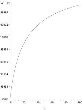
Figure 1: The $g_{tt}$ metric coefficient, for values $\frac{v_{0}^{2}}{c^{2}}=10^{-4}$, $r_{s}=10kpc$.

We can go on and work with the other metric coefficient, $g_{rr}=(1-\frac{2\,G\,M(r)}{c^{2}\,r})^{-1}$. First of all, recall that the $g_{tt}$ coefficient was determined based on the analysis presented above. For the $g_{rr}$ coefficient, the unknown function $M(r)$ can not be directly identified with the mass function. Strictly speaking, the mass is defined for asymptotically flat spacetimes with several characteristics, but we do not go into that discussion in this work. We can say that this is an approximation. On the other hand, however, as will be shown below, the ${}^{t}_{t}$ component of the Einstein equations, implies a consistency between the fact of taking this function as the mass and the defined density, so that we have some grounds to consider it like the mass. Thus, let us be bold and take the function $M(r)$ as the mass function of the NFW model. The line element takes the form:

$$ds^{2}=-\left(1+\frac{r}{r_{s}}\right)^{-2\frac{v_{0}^{2}\,r_{s}}{c^{2}\,r}}\,c^{2}\,dt^{2}+\frac{dr^{2}}{1-2\,\frac{v_{0}^{2}}{c^{2}}\,\left(\frac{\ln\left(1+\frac{r}{r_{s}}\right)}{\frac{r}{r_{s}}}-\frac{1}{1+\frac{r}{r_{s}}}\right)}+r^{2}\,d\Omega^{2},$$ (16)

In this way, we obtain the geometry associated with the Navarro-Frenk-White model.

The line element has two free parameters, namely $v_{0}$, the characteristic speed, and $r_{s}$, the characteristic radius.

With respect to the $g_{rr}$ metric coefficient, it is also regular everywhere, for positive radius, we see its behavior in figure Fig.(2), and it has the following limits:

$$\lim_{r\to 0}g_{rr}=\lim_{r\to\infty}g_{rr}=1.$$ (17)

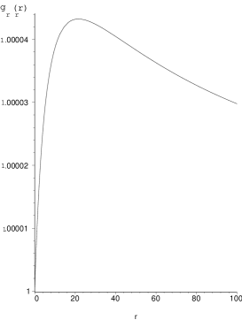
Figure 2: The $g_{tt}$ metric coefficient, for values $\frac{v_{0}^{2}}{c^{2}}=10^{-4}$, $r_{s}=10kpc$.

Thus, the line element given by Eq.(16) is regular at all points and far from the source takes the form of the flat spacetime.

However, even though the line element does not show any divergence, we expect to have one, directly inherited from the divergence of the NFW density at the center. Actually, when one derives the scalar of curvature, $R$, it is seen that:

$$R_{r\to 0}\sim 2\frac{v_{0}^{2}}{c^{2}\,r_{s}\,r}-2\frac{v_{0}^{2}}{c^{2}\,r_{s}^{2}}\left(2-\frac{v_{0}^{2}}{c^{2}}\right)+{\cal O}(r),$$ (18)

showing a clear divergence at the center, as expected. This implies that we do not have a solution describing a spacetime, as long as there is a naked singularity, the divergence is not covered by any horizon. What we have is a geometry which implies a dynamic similar to the one described by the NFW model, so we claim that this geometry will be related with the exterior part of a complete spacetime with the observed dynamics.

The metric coefficients differ from the unity by very tiny amounts, validating the flat space approximation, that is, the Newtonian analysis. However, within the General relativistic theory, these tiny amounts of non-flat geometry, are the ones responsible for the observed dynamics!

Finally, we can construct the Einstein tensor and obtain some conclusions about the type of matter-energy which produce the space time given by Eq.(16). The Einstein tensor gives three non-zero independent components:

$$G^{t}_{t} = -2\frac{v_{0}^{2}}{c^{2}\,r_{s}^{2}}\,\frac{1}{x\,u^{2}},$$ (19)

$$G^{r}_{r} = -4\frac{v_{0}^{4}}{c^{4}\,r_{s}^{2}}\,\frac{1}{x^{4}\,u^{2}}\,\left[u\,\ln u\,\left(u\,\ln u-2\,x\right)+x^{2}\right],$$ (20)

$$G^{\theta}_{\theta} = -\frac{v_{0}^{4}}{c^{4}\,r_{s}^{2}}\,\frac{1}{x^{5}\,u^{3}}\,\left(u\,\ln u-x\right)\,\left[2\,u\,\ln u\,\left(\frac{v_{0}^{2}}{c^{2}}\,u\,\ln u-2\,x\,\left(u+\frac{v_{0}^{2}}{c^{2}}\right)\right)+x^{2}\,\left(7\,x+4+2\,\frac{v_{0}^{2}}{c^{2}}\right)\right],$$ (21)

where we have defined $x=\frac{r}{r_{s}}$, and $u=1+\frac{r}{r_{s}}$.

Being aware of the caveats on promoting this geometry to a spacetime, still we can say something about the type of matter which could produce such a geometry, by means of the Einstein equations:

$$G^{\mu}_{\nu}=\frac{8\,\pi\,G}{c^{4}}\,T^{\mu}_{\nu},$$ (22)

where $G$ stands for the gravitational constant and $T^{\mu}_{\nu}$ describes the tensor of distribution of the matter-energy in the spacetime.

It is common to identify the $T^{t}_{t}$ component of the matter-energy tensor with the density of matter, and energy, present in the spacetime, $\rho$, that is $T^{t}_{t}=-c^{2}\,\rho$. Thus, using the corresponding expression for the Einstein tensor, Eq.(19), we obtain the same expression relating the mass and the density as that obtained in the Newtonian theory, Eq.(12). This fact gives support to the interpretation of the function $M(r)$ in the line element, Eq.(16), as the mass of the system. These are good news and give consistency to the treatment presented here.

About the other components of the matter-energy tensor, by means of the Einstein equations, we can conclude that such matter-energy tensor can not be dust or even perfect fluid. The reason for these conclusions are clear. Again, if we take the matter-energy tensor to be a perfect fluid one

$$T^{\mu}_{\nu}=\left(\rho\,c^{2}+p\right)u^{\mu}\,u_{\nu}+p\,\delta^{\mu}_{\nu},$$ (23)

with $u^{\mu}$ the four velocity. For the spherically symmetric case we are dealing with, the matter-energy tensor takes the form $T^{\mu}_{\nu}={\rm diag}\left(-\rho\,c^{2},p,p,p\right)$. But, from the Einstein tensor, we see that clearly $G^{r}_{r}$, and $G^{\theta}_{\theta}$ are non zero and different. Thus, the matter-energy curving the spacetime to form the NFW geometry can not be dust or perfect fluid.

If we insist on a dark fluid type for the matter-energy, it has to be an anisotropic one, with two different pressures, a radial one, $p_{r}$, and a tangential one, $p_{\bot}$ which, by the Einstein equations imply

$$p_{r} = -\rho^{2}\,2\,\pi\,G\,\frac{r_{s}^{2}\,u^{2}}{x^{2}}\,\left[u\,\ln u\,\left(u\,\ln u-2\,x\right)+x^{2}\right]$$ (24)

$$p_{\bot} = -\rho^{2}\,8\,\pi\,G\,\frac{r_{s}^{2}\,u}{x^{3}}\,\left(u\,\ln u-x\right)\,\left[2\,u\,\ln u\,\left(\frac{v_{0}^{2}}{c^{2}}\,u\,\ln u-2\,x\,\left(u+\frac{v_{0}^{2}}{c^{2}}\right)\right)+x^{2}\,\left(7\,x+4+2\,\frac{v_{0}^{2}}{c^{2}}\right)\right].$$ (25)

It is important to notice that, as the density, $\rho$ is very small, these pressures are even smaller, and tend very quickly to zero. Thus, again validate the Newtonian treatment taken the fluid as dust, in an exterior region. Nevertheless, recall that these analysis is on the track of determining the actual nature of the dark matter, pointing to the physical properties it must have.

In this way, the geometry associated with the NFW model that we have derived, allows us to explain the validity of the Newtonian treatment, pointing to its limits, to discuss on the nature of the dark matter, and opens the road to perform several dynamical studies within the general relativistic theory.

We are grateful with Elloy Ayon for fruitful discussions during the elaboration of the present work. DN acknowledges the DGAPA-UNAM grant IN-122002.

References

- (1) T. Matos, D. Núñez, F. S. Guzmán and E. Ramírez, Gen. Rel. and Grav. 34, 283 (2002).
- (2) F. S. Guzmán, T. Matos, D. Núñez, and E. Ramírez, Rev. Mex. de Fis. to appear, (2003).
- (3) J. F. Navarro, C. S. Frenk, and S. D. M. White, Astrop. J. 490, 493, (1997).