Multi-frequency polarimetry of the Galactic radio background around 350 MHz: I. A region in Auriga around l = 161°, b = 16°

With the Westerbork Synthesis Radio Telescope (WSRT), multi-frequency polarimetric images were taken of the diffuse radio synchrotron background in a $\sim$ 5°$\times$7° region centered on $(l,b)=(161\degr,16\degr)$ in the constellation of Auriga. The observations were done simultaneously in 5 frequency bands, from 341 MHz to 375 MHz, and have a resolution of $\sim$ 5.0′$\times$5.0′ cosec $\delta$. The polarized intensity $P$ and polarization angle $\phi$ show ubiquitous structure on arcminute and degree scales, with polarized brightness temperatures up to about 13 K. On the other hand, no structure at all is observed in total intensity $I$ to an r.m.s. limit of 1.3 K, indicating that the structure in the polarized radiation must be due to Faraday rotation and depolarization mostly in the warm component of the nearby Galactic interstellar medium (ISM). Different depolarization processes create structure in polarized intensity $P$. Beam depolarization creates “depolarization canals” of one beam wide, while depth depolarization is thought to be responsible for creating most of the structure on scales larger than a beam width. Rotation measures ($RM$) can be reliably determined, and are in the range $-17\la RM\la 10$ rad m^-2 with a non-zero average $RM_{0}\approx-3.4$ rad m^-2. The distribution of $RM$s on the sky shows both abrupt changes on the scales of the beam and a gradient in the direction of positive Galactic longitude of $\sim$ 1 rad m^-2 per degree. The gradient and average $RM$ are consistent with a regular magnetic field of $\sim 1\leavevmode\nobreak\ \mu$G which has a pitch angle of $p=-14$°. There are 13 extragalactic sources in the field for which $RM$s could be derived, and those have $|RM|\la 13$ rad m^-2, with an estimated intrinsic source contribution of $\sim$ 3.6 rad m^-2. The $RM$s of the extragalactic sources show a gradient that is about 3 times larger than the gradient in the $RM$s of the diffuse emission and that is approximately in Galactic latitude. This difference is ascribed to a vastly different effective length of the line of sight. The $RM$s of the extragalactic sources also show a sign reversal which implies a reversal of the magnetic field across the region on scales larger than about ten degrees. The observations are interpreted in terms of a simple single-cell-size model of the warm ISM which contains gas and magnetic fields, with a polarized background. The observations are best fitted with a cell size of 10 to 20 pc and a ratio of random to regular magnetic fields $B_{ran}/B_{reg}\approx 0.7\pm 0.5$. The polarization horizon, beyond which most diffuse polarized emission is depolarized, is estimated to be at a distance of about 600 pc.

1 Introduction

The warm ionized gas and magnetic field in the Galactic disk Faraday-rotate and depolarize the linearly polarized component of the Galactic synchrotron emission. Structure of the warm ionized Interstellar Medium (ISM) is imprinted in the polarization angle and polarized intensity by Faraday rotation and depolarization. Therefore, the structure in the polarized diffuse radio background provides unique information about the structure in the magneto-ionized component of the ISM. Using interferometers we can probe arcminute scales, which correspond to linear scales from a fraction of a parsec to several tens of parsecs. Multi-frequency radio polarization observations of the Faraday-rotated synchrotron emission enable determination of the rotation measure ($RM$) distribution along many contiguous lines of sight. Therefore, this is a valuable method to estimate the non-uniform component of the Galactic magnetic field, weighted with electron density.

Although the magnetic field is only one of the factors that shape the very complex multi-component ISM, it is generally thought to play a major rôle in the energy balance of the ISM and in setting up and maintaining the turbulent character of the medium. The non-uniform component of the magnetic field may influence heating of the ISM (Minter & Balser 1997), and provide global support of molecular clouds (e.g. Vázquez-Semadeni et al. 2000, Heitsch et al. 2001). It also plays an important rôle in star formation processes (e.g. Shu 1985, Beck et al. 1996, Ferrière 2001). Furthermore, observations of the detailed structure of the magnetic field can provide constraints for Galactic dynamo models (Han et al. 1997).

The strength and structure of the magnetic field in the warm ionized medium in the Galaxy can also be obtained from Faraday rotation measurements of pulsars, or polarized extragalactic sources.

Among these, radio observations of pulsars take a special place because for them one can measure the $RM$ and the dispersion measure ($DM$) along the same line of sight. The ratio of the two immediately yields the averaged component of the magnetic field along a particular line of sight (see e.g. Lyne & Smith 1989, Han et al. 1999). These studies, and analysis of the distribution of polarized extragalactic sources (e.g. Simard-Normandin & Kronberg 1980, Sofue & Fujimoto 1983), suggest that the regular Galactic magnetic field is directed along the spiral arms, with a pitch angle of $p\approx 5-15$°. There is evidence for reversals of the uniform magnetic field inside the solar circle (e.g. Simard-Normandin & Kronberg 1979, Rand & Lyne 1994), while there is still debate on reversals outside the solar circle (e.g. Vallée 1983, Brown & Taylor 2001, Han et al. 1999). Rand & Kulkarni (1989) used pulsar $RM$s to derive a value for the strength of the regular component of the magnetic field of $B_{reg}=1.3\pm 0.2\leavevmode\nobreak\ \mu$G. This result assumes a circularly symmetric large-scale Galactic magnetic field. The residuals with respect to the best-fit large-scale model were interpreted as due to a random magnetic field of 5 $\mu$G. This number was derived by assuming a scale length of the random field, modeled as a cell size, of 55 pc. Ohno & Shibata (1993) confirmed this result for the random magnetic field component for all cell sizes in the range of 10 - 100 pc. They used 182 pulsars in pairs and therefore did not have to make any assumptions about a large-scale Galactic magnetic field.

Using extragalactic sources, most of which are double-lobed with lobe separations between 30′′ and 200′′, Clegg et al. (1992) found substantial fluctuations in $RM$ on linear scales of $\sim$ 0.1 - 10 pc, which they could explain by electron density fluctuations alone. However, Minter & Spangler (1996) observed $RM$ fluctuations in extragalactic source components that cannot be explained by only electron density fluctuations; they need an additional turbulent magnetic field of $\sim 1\,\mu$G to fit the observations. Observations of polarization of starlight (Jones et al. 1992) give much larger estimates of the cell size, of up to a kpc.

Using pulsars and extragalactic radio sources for the determination of the $RM$ of the Galactic ISM is clearly not ideal, because they only provide information in particular directions which sample the ISM very sparsely. On the contrary, the diffuse Galactic radio background provides essentially complete filling over large solid angles. Therefore, rotation measure maps of the diffuse emission can be produced that give information on the electron-density-weighted magnetic field over a large range of scales. The distribution of polarized intensity, when interpreted as mostly being due to depolarization, can yield estimates of several properties of the warm ISM such as correlation length, ratio of random over regular magnetic field and the distance out to which diffuse polarization can be observed. Early $RM$ maps of the diffuse synchrotron emission in the Galaxy were constructed by Bingham & Shakeshaft (1967) and Brouw & Spoelstra (1976) who confirmed a Galactic magnetic field in the Galactic plane. Junkes et al. (1987) presented a polarization survey of the Galactic plane at $4.9\degr<l<76\degr$ and $|b|<1.5\degr$ showing small-scale structure in diffuse polarization. The existence of polarization filaments at intermediate latitudes, without correlated structure in total intensity $I$, was discovered by Wieringa et al. (1993) at 325 MHz. Polarization surveys have been performed at frequencies from 1.4 GHz to 2.695 GHz (Duncan et al. 1997, Duncan et al. 1999, Uyanıker et al. 1999, Landecker et al. 2001, Gaensler et al. 2001), mostly in the Galactic plane.

In this paper, we discuss the results of multi-frequency observations at low frequencies around 350 MHz of a field in the constellation Auriga, in the second Galactic quadrant ($l=161^{\circ}$, $b=16^{\circ}$). Due to the low frequencies, we probe low rotation measures that are predominant at intermediate and high latitudes. This gives the opportunity to study the high-latitude $RM$ without concrete objects such as HII regions or supernova remnants in the line of sight, and estimate structure in the ISM above the thin stellar disk.

Section 2 contains details of the multi-frequency polarization observations. In Sect. 3, we analyze the observations, in particular the small-scale structure in polarized intensity and polarization angle. Faraday rotation is discussed in Sect. 4, where we also present the map of rotation measure. In Sect. 5, depolarization mechanisms are described that cause the structure in $P$, and the constraints that the observations provide for the parameters that describe the warm ISM. In Sect. 6, the polarization properties of 13 polarized extragalactic point sources found in the Auriga region are discussed. In Sect. 7, we discuss the information that our data provides on the strength and structure of the Galactic magnetic field. Finally, our conclusions are stated in Sect. 8.

2 The observations

We used the Westerbork Synthesis Radio Telescope (WSRT) for multi-frequency polarimetric observations of the Galactic radio background in a field in the constellation of Auriga centered on ($\alpha$, $\delta$) (B1950) = $(6^{h}20^{m},52^{\circ}30^{m})$ ($l=161^{\circ}$, $b=16^{\circ}$). This field was observed in 8 frequency bands between 325 and 390 MHz simultaneously, each with a band width of 5 MHz. Due to radio interference and hardware problems only data in 5 of the 8 bands, viz. those centered on 341, 349, 355, 360, and 375 MHz, could be used.

The region in Auriga was observed in six 12hr periods, which resulted in a baseline increment of 12m. The shortest baseline obtained is 36m, and the longest is 2700m, which gives a maximum resolution of $\sim 1$′. A taper was applied to the $(u,v)$-data to increase the signal-to-noise ratio, so as to obtain a resolution of $5.0\arcmin\times 5.0\arcmin$ cosec $\delta=5.0\arcmin\times 6.3\arcmin$ in all 5 frequency bands. As an interferometer has a finite shortest baseline, it is insensitive to large-scale structure. The shortest spacing of 36m in the WSRT constitutes effectively a high-pass filter for all scales above approximately a degree.

The Auriga region was selected from diffuse polarization maps that were produced as a by-product of the Westerbork Northern Sky Survey (WENSS, Rengelink et al. 1997), which is a single-frequency radio survey at 325 MHz. The WENSS diffuse polarization maps contain several regions of high polarization which show conspicuous small-scale structure in polarized intensity and polarization angle. We reobserved two of those regions at multiple frequencies and with higher sensitivity to obtain rotation measure information. The first region in Auriga is described in this paper, and the other one in a forthcoming paper (Haverkorn et al. 2003a).

The data reduction process is described in detail in Haverkorn (2002), and we only give a brief summary here. The observations were reduced using the newstar data reduction package. Polarized and unpolarized standard calibrator sources were used, where the absolute flux scale at 325 MHz is based on a value of 26.93 Jy for 3C286 (Baars et al. 1977). From this value the flux scales of the other calibrator sources 3C48, 3C147, 3C345, and 3C303 were derived.

As the area to be mapped is larger than the primary beam of the WSRT, the mosaicking technique was used (Rengelink et al. 1997). In this observing mode, the array cycles through a preselected set of pointing positions a number of times during the 12 hour observation period, which reduces the instrumental polarization in between pointing centers to below 1%. For the present region we used 5$\times$7 pointing positions separated by 1.25°. We only discuss the central $\sim 7\degr\times$9° of the observed field of view, as the edges of the mosaic exhibit larger noise due to primary beam attenuation and increased instrumental polarization. Maps were constructed of Stokes parameters $I$, $Q$, $U$, and $V$. From Stokes $Q$ and $U$, polarized intensity $P=\sqrt{Q^{2}+U^{2}}$ and polarization angle $\phi=0.5\arctan(U/Q)$ were derived.

Central position	(l,b) = (161°, 16°)
Size	$\sim$ 7°$\times$9°
Pointings	5$\times$7
Frequencies	341, 349, 355, 360, 375 MHz
Resolution	5.0′$\times$5.0′ cosec $\delta$ = 5.0′$\times$6.3′
Noise	$\sim$ 4 mJy/beam (0.5 K)
Conversion Jy - K	1 mJy/beam = 0.127 K (at 350 MHz)
Spacings	Date	Start time	End time
		(UT)	(UT)
36m	96/02/19	13:36	01:54
48m	95/12/24	17:28	05:41
60m	95/12/31	17:13	05:31
72m	96/01/07	16:37	04:55
84m	96/01/30	14:59	03:12
96m	96/01/09	16:33	04:46

Table 1: Observational details of the Auriga field

To avoid spurious solar emission coming in through polarized side lobes, all observations were done at night, as shown in Table. 1. In addition, the observing period was close to solar minimum and in winter, minimizing ionospheric Faraday rotation. The high polarized brightness that we observe (see Sect. 3.2) indicates that ionospheric Faraday rotation does not vary much during each of the 12hr observations, because if it did, hardly any polarized intensity would have resulted. The differences between the average ionospheric Faraday rotation in the six 12hr observations were determined from several point sources (in the $Q$- and $U$-maps at $\sim 1$′ resolution). The result is shown in Fig. 1 for 4 strong sources and 4 weaker sources. The strong sources have a signal-to-noise $\sigma$ = 2 - 3.5 for an individual 12hr observation, which corresponds to an uncertainty in polarization angle $\sigma_{\phi}\approx 10$°. The signal-to-noise of the weaker sources is $\sigma$ = 1.2 - 1.5 ($\sigma_{\phi}\approx 22$°). From Fig. 1 we conclude that differential Faraday rotation between the six 12hr observations is negligible to within the uncertainties with which it can be measured from the point sources.

We can estimate the $RM$ contribution of the ionosphere from the earth magnetic field and the electron density in the ionosphere. The contribution of the ionospheric Faraday rotation is estimated as follows. The total electron content (TEC) in the ionosphere above Westerbork at night, in a solar minimum, and in winter is minimal: TEC $\approx 2.2\;10^{16}$ electrons m^-2 (Campbell, private communication). The Auriga field at declination $\delta=52.5$° is almost in the zenith at Westerbork at hour angle zero. If we assume a vertical component of the earth magnetic field of 0.5 G towards us, and a path length through the ionosphere of 300 km, the $RM$ caused by the ionosphere is 0.3 rad m^-2 at hour angle zero. At larger hour angles, this is even less. So we expect the rotation measure values given in this paper not to be affected by ionospheric Faraday rotation by more than 0.5 rad m^-2.

Figure 1: Polarization angle variation over six 12hr observations, for 8 extragalactic point sources. Four sources denoted by the solid lines are relatively strong ($\sigma$ = 2 - 3.5 for one 12hr measurement), the dotted lines are sources with $\sigma$ = 1.2 - 1.5. Little angle variation over nights points to constant ionospheric Faraday rotation.

2.1 Missing large scale structure

An interferometer is increasingly insensitive to structure on larger angular scales due to missing small spacings. This means for the WSRT that scales above approximately a degree cannot be detected. The $Q$ and $U$ maps are constructed so that in each mosaic pointing, the map integral of $Q$ and $U$ are zero. This leads to missing large-scale components in $Q$ and $U$, and therefore erroneous determinations of $P$, $\phi$ and $RM$. However, the distribution of $RM$ is broad enough within one pointing. Therefore, the variation in polarization angle is so large that the average $Q$ and $U$ are close to zero, so that missing large-scale components are negligible (Sect. 5).

3 Total intensity and linear polarization maps

3.1 Total intensity

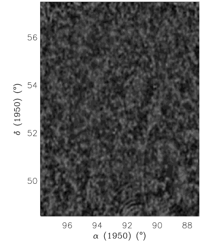
In the left-hand panel of Fig. 2 we show the map of total intensity $I$ at 349 MHz with a resolution of 5.0′$\times$6.3′. Point sources were removed down to the confusion limit of 5 mJy/beam. $I$ has a Gaussian distribution around zero with width $\sigma_{I}=1.3$ K (while the noise, computed from $V$ maps, is $\sigma_{V}=0.5$ K), and is distributed around zero due to the insensitivity of the interferometer to scales $\,\hbox{\hbox to0.0pt{\hbox{\lower 4.0pt\hbox{$\sim$}}\hss} \lower-1.0pt\hbox{$>$}}\,1\degr$. From the continuum single-dish survey at 408 MHz (Haslam et al. 1981, 1982), the $I$-background at 408 MHz in this region of the sky is estimated to be $\sim$ 33 K with a temperature uncertainty of $\sim$ 10% and including the 2.7 K contribution of the cosmic microwave background. Assuming a temperature spectral index of $-2.7$, the backgrounds at the lowest (341 MHz) and the highest (375 MHz) frequency of observation are $\sim$ 49 K and $\sim$ 38 K, respectively. Of these, approximately 25% is due to sources, as estimated from source counts (Bridle et al. 1972), and assuming the spectral index of the Galactic background and the extragalactic sources to be identical. We thus estimate the temperatures of the diffuse Galactic background at 341 and 375 MHz to be 37 and 29 K, respectively.

3.2 Polarized intensity

In the right-hand panel of Fig. 2 we show the map of polarized intensity at 349 MHz, with a resolution of 5.0′$\times$6.3′. The noise in this map is $\sim$ 0.5 K, and the polarized brightness temperature goes up to $\sim$ 13 K, with an average value of $\sim$ 2.3 K.

The map shows cloudy structure of a degree to a few degrees in extent, with linear features that are sometimes parallel to the Galactic plane. In addition, a pattern of black narrow wiggly canals is visible (see e.g. the canal around ($\alpha$, $\delta$) = (92.7^∘, 49^∘ - 51^∘)). These canals are all one synthesized beam wide and are most likely due to beam depolarization. They separate regions of fairly constant polarization angle between which the difference in polarization angle is approximately 90° ($\pm\,n\,180$°, $n=1,2,3\ldots$) (Haverkorn et al. 2000). A change of 90^∘ (or 270^∘, 450^∘ etc.) in polarization angle within one beam cancels the polarized intensity in the beam; therefore these canals appear black in Fig. 2. Hence, the canals are not physical structures, but the reflection of specific features in the distribution of polarization angle. Such canals have also been detected by others at higher frequencies (e.g. Uyanıker et al. 1999, Gaensler et al. 2001). It must be appreciated that the canals represent an extreme case of beam depolarization. Beam depolarization is much more wide-spread if the polarization angle varies on the scale of the beam or on smaller scales, but in general its effect is (much) less than in the canals. Therefore, with the exception of the canals, beam depolarization does not leave easily visible traces in the polarized intensity distribution.

An alternative explanation for depolarized regions accompanied by a change in polarization angle of 90°is so-called depth depolarization or differential Faraday rotation. If the magnetic field in the medium is uniform, depolarization along the line of sight causes depolarized regions at certain $RM$ values (Sokoloff et al. 1998). However, in this scenario, it is hard to explain why the canals are all exactly one beam wide. Furthermore, the canals should shift in position with frequency, which is not observed. For an extended discussion on the possible causes of polarization canals, see Haverkorn et al. 2003b.

Figure 2: Map of the total intensity $I$ (left) and polarized intensity $P$ (right) at 349 MHz, on the same brightness scale. The maps are smoothed to a resolution of $5.0^{\prime}\times 6.3^{\prime}$. White denotes high intensity, up to a maximum of $\sim$ 13 K. Superimposed in the right map are lines of constant Galactic latitude, at latitudes of 13°, 16° and 19°.

There is no obvious structure in Stokes I, and if there is any, it does not appear to be correlated with the structure in P. This is not typical for the Auriga field, but it is true in all fields observed so far with the WSRT at $\sim$ 350 MHz (Katgert & de Bruyn 1999, Haverkorn et al. 2003a, Schnitzeler et al. in prep).

We have estimated the amount of correlation between total and polarized intensity by deriving the correlation coefficient $C$, where $C(f,g)$ of the observables $f(x,y)$ and $g(x,y)$ is defined as

$$C(f,g)=\frac{\sum_{i,j}(f_{ij}-\overline{f})\;(g_{ij}-\overline{g})}{\sqrt{\sum_{i,j}(f_{ij}-\overline{f})^{2}\;\sum_{i,j}(g_{ij}-\overline{g})^{2}}}$$ (1)

where $\overline{f}$ is the average value of $f(x,y)$, $f_{ij}=f(x_{i},y_{j})$, summation is over $i=1,N_{x}$ and $j=1,N_{y}$, and $N_{x}$ and $N_{y}$ is the number of data points in the $x$- and $y$-directions, respectively. The correlation coefficients between $P$ and $I$, and between $P$ and between $I$ at different frequencies are given in Table 2. Both the observed correlation coefficients at the maximum resolution of about 1′, as well as those of the 5′ resolution data are given.

Table 2: Correlation coefficients for correlations between $P$ and $I$, between $I$ in different frequency bands and between $P$ in different frequency bands, for tapered data and full resolution data.

freq band k	res	$C(I_{k},P_{k})$	$C(P_{341},P_{k})$	$C(I_{341},I_{k})$
(MHz)	( ′ )
341	5	–0.008	1.00	1.00
349	5	–0.008	0.67	0.45
355	5	–0.011	0.65	0.34
360	5	0.002	0.58	0.31
375	5	0.015	0.53	0.24
341	1	0.007	1.00	1.00
349	1	0.004	0.60	0.08
355	1	0.0004	0.60	0.21
360	1	0.0002	0.53	0.15
375	1	0.005	0.50	0.16

The high correlations between $I$ in different frequency bands are expected if the visible structure in $I$ is mostly due to faint sources. The $C(I,I)<1$ is due to uncorrelated noise. However, the correlation between $P$ and $I$ is very low, so the structure in polarization is not due to small-scale variations in synchrotron emission. Instead, the variations in polarized intensity and polarization angle must be due to a combination of two processes: Faraday rotation and depolarization. We will return to these in Sects. 4 and 5.

Figure 3: Five maps of a part of the Auriga region at frequencies 341, 349, 355, 360 and 375 MHz. The grey scale is polarized intensity $P$, oversampled 5 times, where white is high intensity. Maximum $P$ (in the 375 MHz band) is approximately 13 K. Superimposed are polarization pseudo-vectors, where each line denotes an independent synthesized beam.

3.3 Polarization angle

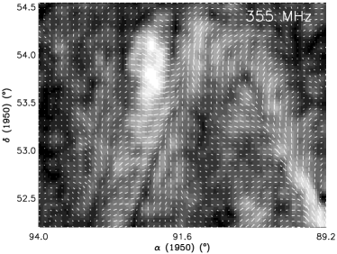
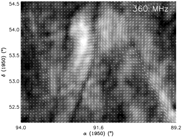
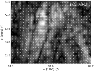
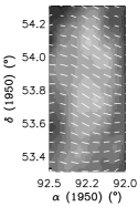
In Fig. 3 we show, for a 3°$\times$2° subfield slightly northwest of the center of the mosaic, maps of polarized intensity $P$ (grey scale) and polarization angle $\phi$ (superimposed pseudo-vectors) in the 5 frequency bands. In the grey scale, which has 5 samples per linear beam width, white corresponds to high $P$. The length of the vectors (one per beam) scales with polarized intensity. The amount of structure in polarization angle is highly variable. At high polarized intensities, the polarization angles mostly vary quite smoothly. However, there are also abrupt changes on the scale of a beam, the most conspicuous of which give rise to the depolarization canals.

Figure 4: Two typical parts of 3$\times$5 beams in the observed field, represented in small graphs of polarization angle $\phi$ against $\lambda^{2}$, one graph per independent synthesized beam. The left 3$\times$5 graphs are taken from a part of the field with high polarized intensity ($\sigma\,\hbox{\hbox to0.0pt{\hbox{\lower 4.0pt\hbox{$\sim$}}\hss} \lower-1.0pt\hbox{$>$}}\,15$ per frequency band), the right part from a region of lower intensity ($\sigma\approx$ 5). The values within parentheses above each graph are $RM$ and reduced $\chi^{2}$, respectively. In general, $RM$s are more regular and alike over several beams in high polarized intensity regions, but there is coherence in $RM$ in lower $P$ regions as well.

4 Faraday rotation

4.1 The derivation of rotation measures

The rotation measure ($RM$) of the Faraday-rotating material follows from $\phi(\lambda^{2})\propto RM\,\lambda^{2}$. As $\phi=0.5\,\arctan(U/Q)$ , the values of polarization angle are ambiguous over $\pm n\,180^{\circ}$ ($n=1,2,3,\ldots$) because a value of angle($Q,U$) is ambiguous over $\pm n\,360^{\circ}$. For most beams, it was possible to obtain a linear $\phi(\lambda^{2})$-relation by using angles with a minimum angle difference between neighboring frequency bands. Only in about 1% of the data, addition or subtraction 180° to the polarization angle in at least one of the frequency bands was needed. One could increase $RM$s by adding or subtracting multiples of 180°, but that would lead to $RM$s in excess of 100 rad m^-2. If such high $RM$s were real, bandwidth depolarization (see Sect. 5) would have totally annulled any polarized signal. In addition, the $RM$s we obtain using the criterion of minimum angle differences (of order of 10 rad m^-2) were also obtained in other observations in this direction (Bingham & Shakeshaft 1967, Spoelstra 1984). So we conclude there are hardly any 180°-ambiguities in polarization angle and we use the minimum angle difference between frequency bands to determine $RM$s.

In Fig. 4 we show $\phi(\lambda^{2})$-plots for small arrays of contiguous, independent beams in typical subfields of the 5′-resolution map. In parentheses are the values of the $RM$ and the reduced $\chi^{2}$ of the linear $\phi(\lambda^{2})$-fit. The leftmost 3$\times$5 plots are from a region with high $P$ ($\sigma\,\hbox{\hbox to0.0pt{\hbox{\lower 4.0pt\hbox{$\sim$}}\hss} \lower-1.0pt\hbox{$>$}}\,$ 15 in all frequency bands), while the rightmost plots are from a region with lower $P$ ($\sigma\approx 5$). In general, the $\phi(\lambda^{2})$-relation is closer to linear in high $P$ regions than in lower $P$ regions, but in the larger part of the Auriga field $RM$s are very well-determined.

4.2 The distribution of rotation measures

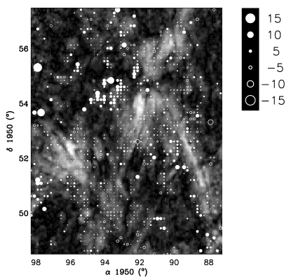
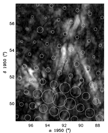
The $RM$s in the Auriga-field are plotted as circles in Fig. 5. Filled circles denote positive values, open circles negative, and the diameters of the circles are proportional to $RM$. For clarity, we only show the $RM$s for one in four independent beams. In addition, $RM$s are only shown when they were reliably determined, i.e. for the average polarized intensity $\left<P\right>>5\sigma$, and for reduced $\chi^{2}$ of the fit $<2$.

The left panel shows $RM$ as determined from the observations. Most $RM$s are negative; the few positive values occur for $\delta\la 52$°, while the largest negative values occur for $\delta\,\hbox{\hbox to0.0pt{\hbox{\lower 4.0pt\hbox{$\sim$}}\hss} \lower-1.0pt\hbox{$>$}}\,55$°. We modeled this systematic variation by a large-scale linear gradient, and find a gradient of about 1 rad m^-2 per degree, with the steepest slope along position angle (from north through east) of $-20\degr$.

The average $RM$, i.e. the $RM$ value in the center of the fitted $RM$-plane, over the field is $RM_{0}\approx-3.4$ rad m^-2. Subtracting the best-fit gradient from the $RM$ distribution yields the $RM$s shown in the right-hand panel in Fig. 5 with only small-sale structure in $RM$. The distribution of small-scale $RM$s (i.e. $RM$ where the large-scale gradient is subtracted) is significantly narrower than the total $RM$ distribution ($\sigma_{\scriptscriptstyle\rm RM}$= 1.4 K instead of 2.3 K), and is more symmetrical, as is shown in Fig. 6, where the two histograms are compared.

The decomposition of the $RM$-distribution into a constant component, a gradient, and a small-scale component is not physical, as there is probably structure on all scales. However, for our purpose it is a good approximation, and it allows us to estimate the large-scale and random components of the Galactic magnetic field, see Sect. 7.

Figure 5: Rotation measures given as circles with a diameter proportional to the magnitude of the $RM$, superimposed over $P$ at 349 MHz in grey scale. The scaling is in rad m^-2. $RM$s are only shown if $P>5\sigma$ and reduced $\chi^{2}<2$, and in both directions, only every second independent beam is plotted for clarity. The right map shows the same data where the best-fitting linear gradient in $RM$ is subtracted.

Figure 6: Histogram of $RM$s in the Auriga field. The dashed line gives the distribution of all “reliably determined” $RM$s, i.e. where $P>5\sigma$ and reduced $\chi^{2}<2$. The solid line gives the reliably determined $RM$ distribution after subtracting a best-fit linear $RM$ gradient from the data. Dotted lines show Gaussian fits to the two histograms.

4.3 Structure in $RM$ on arcminute scales

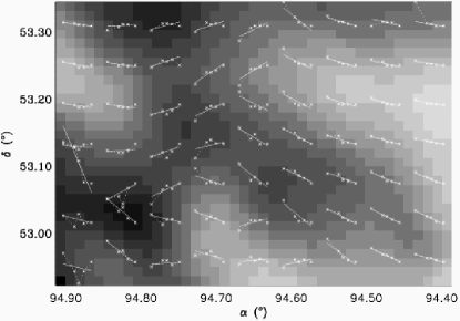
Although the $RM$-distribution shows structure on many scales, the most intriguing changes occur on the scale of the beam, as illustrated in Fig. 7. In the figure, we display a 9$\times$7 array of $\phi(\lambda^{2})$-plots, overlaid on a grey scale representation of $P$ at 349 MHz. Although $RM$ varies quite smoothly over most of the area, there are also abrupt changes, which frequently involve a change of the sign of $RM$ (e.g. at $(\alpha,\delta)=$ (94.60, 53.00)° or (94.68, 53.20)°). Abrupt $RM$ changes over one beam with the right magnitude to cause an angle change of $\pm(n+1/2)\;180$° cause depolarization canals. As $RM$ is an integral over the entire line of sight, it is difficult to understand such changes in $RM$ as resulting from structure in the magnetic field and/or distribution of electrons. As a matter of fact, numerical simulations of the warm ISM show that beam depolarization can enhance $RM$ differences and greatly steepen the gradient (Haverkorn 2002). In addition, models of a medium that produces Faraday rotation and that emits synchrotron radiation show that the $RM$ can change sign without a corresponding change in the direction of the magnetic field (Sokoloff et al. 1998, Chi et al. 1997).

Figure 7: White symbols and lines are plots of $\phi$ against $\lambda^{2}$ and their linear fits, one for each independent beam, so that the slope is $RM$. Sudden $RM$ changes occur over one beam width. The grey scale is polarized intensity at 349 MHz oversampled by a factor of 5. Maximum $P$ (lightest grey) is $\sim$ 40 mJy/beam, while in the bottom left pixel $P$ is set to zero for comparison.

5 The structure in $P$, and the implied properties of the ISM

As $I$ and $P$ are uncorrelated, the structure in $P$ cannot be caused by structure in emission, but instead is created by several instrumental and/or depolarization effects. We discuss these processes in detail in two forthcoming papers for several fields of observation, among which the Auriga field (Haverkorn et al. 2003b,c). Here we summarize them, and discuss the results for the Auriga region.

Structure in $P$ could be induced by the insensitivity of the WSRT to large-scale structure, as a result of missing short-spacing information. However, it is very unlikely that this effect is important in the Auriga observations, because the distribution of $RM$s per pointing center is too wide to allow offsets. If the distribution of $RM$s in a Faraday screen is too wide, the distributions of $Q$ and $U$ of a polarized background that is Faraday-rotated by the screen have averages very close to zero (even if the background was uniformly polarized). As a result, the missing short-spacing information does not produce offsets. For our frequencies the latter is true if $\sigma_{RM}\,\hbox{\hbox to0.0pt{\hbox{\lower 4.0pt\hbox{$\sim$}}\hss} \lower-1.0pt\hbox{$>$}}\,1.8$ rad m^-2. In the Auriga region, this condition is met in essentially all of the subfields of the mosaic. Furthermore, a test in which offsets are added (described in the papers referred to above) to produce better linearity of the $\phi(\lambda^{2})$-relation, did not result in reliable non-zero offsets.

Structure in $P$ could also be generated by non-constant, but high, $RM$ values as a result of bandwidth depolarization. Summation of polarization vectors with different angles in a frequency band will reduce the polarized intensity. The amount of depolarization depends on the spread in polarization angle within the band which, in turn, depends on the $RM$ and the width of the frequency band. For the $RM$s of order 10 rad m^-2 and our bandwidth of 5 MHz the effect is negligible.

A special kind of structure in $P$ is due to beam depolarization, viz. the cancellation of polarization by vector summation across the beam defined by the instrument. This is a 2-dimensional summation of polarization vectors across the plane of the sky, which is probably responsible for the depolarization canals. It certainly cannot produce all of the structure in $P$ because it occurs on a single, small scale, whereas $P$ has structure on a large range of scales.

Finally, depth depolarization occurs along the line of sight in a medium that both emits synchrotron radiation and produces Faraday rotation. It must be responsible for a large part of the structure in $P$. The ISM in the Galactic disk most likely is such a medium. The Galactic synchrotron emission has been modeled by Beuermann et al. (1985) as the sum of two contributions: the thin disk with a half equivalent width of $\sim$ 180 pc, which coincides with the stellar disk, and a thick disk of half equivalent width $\sim$ 1800 pc (where the galactocentric radius of the sun is assumed $R_{\odot}=10$ kpc). Thermal electrons exist also out to a scale height of approximately a kpc, contained in the Reynolds layer (Reynolds 1989, 1991). So up to a height of about a kpc, the medium probably consists of both emitting and Faraday-rotating material. In such a medium, the polarization plane of the radiation emitted at different depths is Faraday-rotated by different amounts along the line of sight. Therefore the polarization vectors cancel partly, causing depolarization along the line of sight even if the magnetic field and thermal and relativistic electron densities are constant (differential Faraday rotation, see Gardner & Whiteoak 1966, Burn 1966, Sokoloff et al. 1998). If the medium contains a random magnetic field, the polarization plane of the synchrotron emission will vary along the line of sight causing extra depolarization in addition to the differential Faraday rotation (called internal Faraday dispersion). We will refer to the combination of the two mechanisms along one line of sight as depth depolarization, thus adopting the terminology proposed by Landecker et al. (2001).

Depth depolarization is the dominant depolarization process in the Auriga field. We constructed a numerical model in Haverkorn et al. (2003c) to evaluate if depth depolarization can indeed be held responsible for most of the structure in $P$, in the Auriga region as well as in the other region that we studied. At the same time, the model makes it possible to estimate the conditions in the warm component of the ISM. The model consists of a layer corresponding to the thin Galactic disk, where random magnetic fields on small scales are present, and a constant background polarized radiation.

In the model, the thin disk (with height $h$) is divided in cells of a single size $d$, which contain a random magnetic field component $B_{ran}$ and a regular magnetic field $B_{reg}$. The amplitude of $B_{ran}$ is constant, but in each cell its direction is randomly chosen. Each cell emits synchrotron radiation, proportional to $B_{\perp}^{2}=(B_{ran,\perp})^{2}+(B_{reg,\perp})^{2}$, where we add energy densities because the two components are physically separated different fields. Only a fraction $f$ of the cells contains thermal electrons, and therefore Faraday-rotates all incoming radiation (to represent the filling factor $f$ of the warm ISM).

We distinguish several kinds of model parameters. First, we have input parameters with values taken from the literature; these are thermal electron density $n_{e}=0.08$ cm^-3, filling factor $f=0.2$ (both from Reynolds 1991), and height of the Galactic thin disk $h=180$ pc (Beuermann et al. 1985). Secondly, there are constraints from the observations of the Auriga field, viz. the width, shape and mean of the $Q$, $U$, $I$ and $RM$ distributions. In addition, we define parameters without observational constraints, such as cell size $d$ and emissivity per cell, which we vary in a attempt to constrain them from the model given the observational constraints. Finally, there are parameters that can be adjusted and optimized for each allowed cell size and emissivity per cell, like the random and regular magnetic field components and background intensity.

Using the observations of the Auriga region to constrain the parameters in the depth depolarization model, we obtain the following estimates. The cell size $d$ is probably in the range from 5 - 20 pc, the random component of the magnetic field $B_{ran}$ is about 1 $\mu$G for a cell size of 5 pc or larger, and up to 4 $\mu$G for smaller cell sizes. With the estimate of the large-scale, regular field ($\sim$ 3 $\mu$G) this leads to a value of about 0.3 to 1.3 for $B_{ran}/B_{reg}$. This is lower than most other estimates of $B_{ran}/B_{reg}$ in the literature, which seem to indicate a value larger than 1. One possible explanation for this discrepancy is the fact that the Auriga region is not very large. Therefore random magnetic field components that project to angular scales larger than a few degrees will have been interpreted as components of the regular field. If such large-scale random components exist, this effect will artificially decrease $B_{ran}/B_{reg}$. Secondly, the Auriga field was selected for its conspicuous polarization structure, and high polarized intensity in general indicates a more regular magnetic field structure. Finally, the Auriga region is observed in an inter-arm region. The next spiral arm, the Perseus arm, is more than 2 kpc away, and we expect that at these frequencies, all polarized emission from the Perseus arm is depolarized. There are indications that in the inter-arm region, the regular magnetic field component is higher than the random magnetic field component (Han & Qiao 1994, Indrani and Deshpande 1998, Beck 2001).

A cell of size 10 pc located at the far edge of the thin disk still subtends a little less than a degree in our maps. We see structure on smaller scales, so that cells of approximately a parsec have to be present as well. Indeed, there are many indications that structure exists in the ISM on many scales (Armstrong et al. 1995, Minter & Spangler 1996).

The distance out to which polarized radiation is not depolarized by depth depolarization, as derived from the model, is shown in Fig. 8.

Figure 8: The amount of polarization contributed by a certain cell, against the distance to that cell, in a single-cell-size model of polarized radiation propagating through a magneto-ionized medium.

The total path length through the medium containing small-scale structure was about 600 pc, which corresponds to a height of the thin disk of about 150 pc for the Auriga latitude of $\sim$ 16°. Radiation emitted at large distances is depolarized more than emission from nearby, but there is no definite polarization horizon due to depth depolarization. Beam depolarization can cause a polarization horizon, as structure further away will be on smaller angular scales, which causes more beam depolarization (Landecker et al. 2001).

6 Polarized extragalactic point sources

Table 3: Extragalactic sources in the Auriga region. The second column gives position, and the third $RM$s. Reduced $\chi^{2}$ of the $\phi(\lambda^{2})$ relation is given in column 4. Columns 5, 6 and 7 give resp. $P$, $I$ (both in mJy/beam) and percentage of polarization $p$ averaged over the five frequency bands.

$$\begin{array}[]{rrrrrrr}\hline\cr\vskip 3.0pt plus 1.0pt minus 1.0pt\cr\mbox{No.}&(\alpha,\delta)\;(\;\degr,\;\degr)&\lx@intercol\hfil RM\;\mbox{(rad\leavevmode\nobreak\ m${}^{-2}$)}\hfil\lx@intercol&\lx@intercol\hfil\;\;\;\chi^{2}\hfil\lx@intercol&\lx@intercol\hfil\;\;\left<P\right>\hfil\lx@intercol&\lx@intercol\hfil\;\;\left<I\right>\hfil\lx@intercol&\lx@intercol\hfil\;\;\left<p\right>\hfil\lx@intercol\\ \vskip 3.0pt plus 1.0pt minus 1.0pt\cr\hline\cr\vskip 3.0pt plus 1.0pt minus 1.0pt\cr 1&\mbox{[ 97.9, 55.3 ]}&7.4\pm 0.2&\hskip 8.5359pt12.9&45.6&2021&2.3\\ 2&\mbox{[ 97.7, 53.6 ]}&12.9\pm 0.3&\hskip 8.5359pt3.1&14.9&216&6.9\\ 3&\mbox{[ 96.6, 53.3 ]}&6.6\pm 0.4&\hskip 8.5359pt1.7&15.0&224&6.7\\ 4&\mbox{[ 96.5, 54.1 ]}&5.7\pm 0.4&\hskip 8.5359pt3.7&11.9&380&3.1\\ 5&\mbox{[ 95.3, 50.8 ]}&0.6\pm 0.4&\hskip 8.5359pt1.6&14.7&165&8.8\\ 6&\mbox{[ 95.2, 50.8 ]}&3.1\pm 0.4&\hskip 8.5359pt0.2&14.7&197&7.5\\ 7&\mbox{[ 94.7, 54.8 ]}&7.9\pm 0.3&\hskip 8.5359pt3.0&18.8&282&6.7\\ 8&\mbox{[ 93.4, 55.6 ]}&6.3\pm 0.2&\hskip 8.5359pt1.1&21.3&180&11.8\\ 9&\mbox{[ 92.3, 52.9 ]}&2.7\pm 0.1&\hskip 8.5359pt6.1&35.8&1222&2.9\\ 10&\mbox{[ 90.3, 50.4 ]}&-10.2\pm 1.4&\hskip 8.5359pt4.4&7.4&168&4.4\\ 11&\mbox{[ 89.3, 55.0 ]}&3.0\pm 0.4&\hskip 8.5359pt1.4&11.6&340&3.4\\ 12&\mbox{[ 89.2, 52.5 ]}&-8.1\pm 0.1&\hskip 8.5359pt12.7&22.1&477&4.6\\ 13&\mbox{[ 89.0, 52.3 ]}&-13.6\pm 0.4&\hskip 8.5359pt5.8&14&237&5.9\\ \vskip 3.0pt plus 1.0pt minus 1.0pt\cr\hline\cr\end{array}$$

Thirteen polarized extragalactic point sources in the Auriga-field were selected based on three selection criteria: (1) signal-to-noise $\sigma>3$ in $P$ at all frequencies, (2) the degree of polarization $p$ is higher than 1% at all frequencies (because a lower polarization degree can also be caused by instrumental polarization, see Sect. 2), and (3) the source does not lie too far at the edge of the field away from any pointing center, to limit the contribution from instrumental polarization. The 13 sources are all detected in the 1′ resolution data, and most of them are unresolved at that resolution. Their $RM$s vary from approximately –13 to 13 rad m^-2.

The relevant properties of the sources are given in Table 3, where the second column gives the right ascension and declination, column 3 the $RM$, and column 4 the reduced $\chi^{2}$ of the $\phi(\lambda^{2})$-fits. Columns 5, 6, and 7 give the values of $P$, $I$ and percentage of polarization $p$ respectively, averaged over all frequency bands.

Figure 9: Plots of polarization angle $\phi$ against $\lambda^{2}$ for the 13 polarized extragalactic sources in Table 3. Note that the scaling of the $\phi$-axis differs for each source.

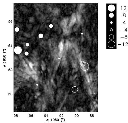
Fig. 9 shows the polarization angle $\phi$ plotted against $\lambda^{2}$ for each point source. In Fig. 10, we show the 13 sources overlaid on a grey scale plot of polarized intensity at 349 MHz, with their $RM$s indicated. The diameter of the symbol and its shading indicate the value of $RM$.

Sources 1 and 2 could have a significant contribution of instrumental polarization, because they are observed in only one pointing center and are located about 0.8° to 1° away from the pointing center. Nevertheless, they show linear $\phi(\lambda^{2})$-relations, which indicates that instrumental polarization is not important. These sources are therefore included in the analysis.

Figure 10: $RM$s of the 13 polarized extragalactic point sources in the Auriga field in circles, overlaid on $P$ at 349 MHz. Filled circles are positive $RM$s, open circles negative. The crosses denote the pointing centers, and the scaling is in rad m^-2.

The strong correlation of $RM$ across the sky indicates a Galactic component to the $RM$s of the extragalactic point sources. The best-fitting linear gradient to the $RM$s of the sources has a steepest slope of 3.62 rad m^-2 per degree in position angle 72°, i.e. roughly in the direction of increasing Galactic latitude (position angle 66°). The standard deviation of $RM$s around this gradient is $\sigma_{RM}\approx 3.6$ rad m^-2. This is consistent with the result of Leahy (1987), who finds a typical ’internal’ $RM$ contribution from the extragalactic source or a halo around it of $\sim$ 5 rad m^-2.

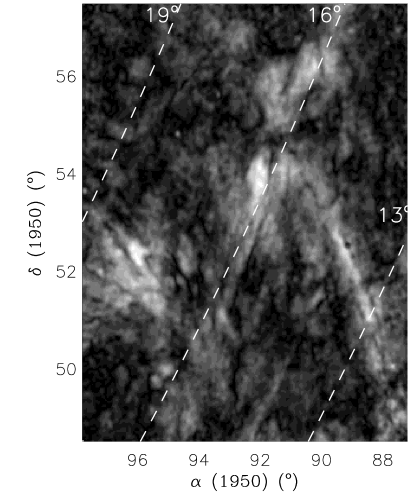
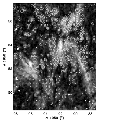
The change of sign of $RM$ of the extragalactic sources within the observed region indicates a reversal in the Galactic magnetic field. (Unlike the diffuse emission, sign changes in $RM$s of extragalactic sources cannot be due to depolarization effects.) The reversal exists on scales larger than our field of view, as is shown in Fig. 11, where we combine the $RM$s of our sources with those from the literature. The circles are our sources, the squares indicate sources that were detected by Simard-Normandin et al. (1981) and/or by Tabara & Inoue (1980), and the one triangle indicates the only pulsar nearby (Hamilton & Lyne 1987). The numbers next to the squares and triangle give the magnitude of $RM$ of the source (the diameter of the symbol is only proportional to $RM$ up to $RM$ = 15 rad m^-2). One source at $(\alpha,\delta)=(91.25\degr,48\degr)$ was omitted, because Simard-Normandin et al. give $RM$ $=34$ rad m^-2 and Tabara & Inoue give $RM$ $=-64.9$ rad m^-2.

Figure 11: $RM$s of extragalactic point sources and of one pulsar. The circles are the point sources detected in the Auriga field, where the radius of the circle is proportional to the magnitude of $RM$. Squares are extragalactic point sources detected by Simard-Normandin et al. (1981) and/or by Tabara & Inoue (1980), and the one triangle in the field denotes the only pulsar near the Auriga field (Hamilton & Lyne 1987). Values of the $RM$ are written next to the sources, and for $RM$ $<15$ rad m^-2 the radius of the symbol is proportional to $RM$.

The source distribution shows a clear magnetic field reversal, which is not on Galactic scale but on smaller scales, as is shown in Figs. 1 and 2 of Simard-Normandin & Kronberg (1980), which show $RM$s of extragalactic sources over the whole sky.

The gradient in $RM$ measured in the extragalactic point sources is completely unrelated and almost perpendicular to the structure in $RM$ from the diffuse emission. This can be explained from the widely different path lengths that extragalactic sources and diffuse emission probe. Diffuse emission can only be observed out to a distance of a few hundred pc to a kpc, as radiation from further away will be mostly depolarized. On the contrary, extragalactic sources are Faraday-rotated over the complete path length through the Milky Way of many kiloparsecs long. Therefore, the $RM$ structure from diffuse radiation and from extragalactic sources gives information about different regions in the Galaxy.

7 Discussion

7.1 High $P$-structures and alignment with the Galactic plane

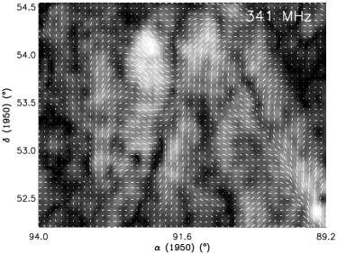
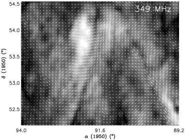
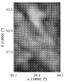
The depth depolarization model described in Sect. 5 only describes the properties of the ISM in a statistical manner, by giving a representation of an average line of sight. Therefore, it does not pretend to give a detailed description of the distribution of $P$, as it is actually observed. Even the global properties of the $P$ distribution, like the general alignment with the Galactic plane, is not part of the model. This alignment is not only visible in the Auriga field, but also in other regions observed with the WSRT (Haverkorn et al. 2003a, Schnitzeler et al. in prep). The large-scale structures in $P$ cannot be caused by substantial extra emission, because that should be accompanied by corresponding structure in $I$, which is not observed. Instead, where the polarized intensity is highest, the depolarization is probably the least, so that there the ISM is relatively transparent to polarized emission. In general, high depolarization is caused by a large amount of structure in $RM$, along the line of sight and/or over the sky (the latter on the scale of the beam or smaller). This explanation of the structure of high $P$ is borne out by the relation between polarized intensity $P$ and $\sigma_{\scriptscriptstyle\rm RM}$, shown in Fig. 12. This figure shows the width $\sigma_{\scriptscriptstyle\rm RM}$ of a Gaussian fit to the $RM$ distribution in several intervals of polarized intensity with a width $\Delta P=0.01$ Jy/beam. Rotation measure clearly varies more at lower polarized intensity, where only well-determined $RM$s are used so that the effect cannot be due to noise. For the two intervals of highest $P$ (0.08 – 0.09 Jy/beam and 0.09 – 0.10 Jy/beam), not shown in Fig. 12, no Gaussian fit could be made, as the distributions were bimodal. The peaks in these bimodal distributions correspond to two spatially coherent structures, which are shown in the two panels of Fig. 13. In the region around $(\alpha,\delta)=(94.6\degr,51.8\degr)$, $-1.5\la RM\la 0$ rad m^-2, while in the region around $(\alpha,\delta)=(92.2\degr,53.8\degr)$, $0\la RM\la 1.3$ rad m^-2. Clearly, $RM$ is indeed very uniform in regions of high polarization. The low variation in $RM$ is also reflected in the uniformity of the polarization angles.

Figure 12: Width of a Gaussian fit to the $RM$ distribution $\sigma_{\scriptscriptstyle\rm RM}$ for a range of $P$, where $P$ is divided in bins of 0.01 Jy/beam.

Figure 13: Two areas in the $P$ map at 349 MHz with highest $P$ ($>80$ mJy/beam). Overlaid pseudo-vectors are polarization angles, showing a minimal change in angle for high $P$.

A constant $RM$ over a certain area sets an upper limit on structure in magnetic field and thermal electron density. The fact that some of the filamentary structure in $P$ is aligned with Galactic latitude suggests a magnetic origin, although stratification of $n_{e}$ over Galactic latitude can contribute as well. For variation of polarization angle over the filament of less than about 20° (from Fig. 13), $\Delta RM$ $\la 0.5$ rad m^-2 is needed. If magnetic field structure would be the same over the entire path length towards the filament, and assuming $n_{e}=0.08$ cm^-3, this requires a magnetic field change $\Delta B_{\parallel}\la 0.01\leavevmode\nobreak\ \mu$G with a polarization depth of 600 pc. Even if the filamentary structures are sheet-like with a constant magnetic field over a large part of the path length, or if the polarization horizon is locally much shorter than the highly uncertain value of 600 pc, the upper limit to $\Delta B$ is very low. Therefore, this structure of high $P$ aligned with Galactic latitude indicates the existence of long filaments or sheets parallel to the Galactic plane of highly uniform magnetic field and thermal electron density. As back- and/or foreground structure can also imprint structure in $RM$, these regions may well be characterized by low thermal electron density.

7.2 The Galactic magnetic field

The Auriga field of 7°$\times$9° represents only 0.1% of the sky, and is therefore by itself not very well suited for an analysis of the global properties of the Galactic magnetic field. However, we can estimate strength and direction of the regular component of the Galactic magnetic field from the distribution of $RM$s of the diffuse radiation and of the extragalactic sources over the field.

First, we need to determine how much of the $RM$ gradient seen in the diffuse emission is caused by $n_{e}$, and how much by $B_{\parallel}$. Independent measurements of $n_{e}$ can be obtained from the emission measure $EM=\int n_{e}^{2}\;dl$, as measured with the Wisconsin H$\alpha$ Mapper survey (WHAM, Haffner et al., in prep, Reynolds et al. 1998), shown in Fig. 14. As the resolution is about a degree, the WHAM survey cannot be used to determine small-scale structure in $n_{e}$, but gives an estimate of the global gradient in $n_{e}$ over the field. From north to south, the H$\alpha$ observations show an increase from about 1 to 5 Rayleighs (1 Rayleigh is equal to a brightness of $10^{6}/4\pi$ photons cm^-2 s^-1 ster^-1, and corresponds to an $EM$ of about 2 cm^-6 pc for gas with a temperature T = 10000 K). The small enhancement in $EM$ at $(\alpha,\delta)=(94.8\degr,55.5\degr)$ is probably related to the ancient planetary nebula PuWe1 (PW1, Tweedy & Kwitter 1996). Note that the H$\alpha$ emission probes a longer line of sight than the diffuse polarization, and is velocity integrated over $-$80 to 80 km s^-1 LSR, so complete correspondence is not expected. However, a gradient in $RM$ that was solely due to the $n_{e}$-gradient would have a sign opposite to that of the observed $RM$-gradient. Therefore, the observed gradient in $RM$ must be due to a gradient in the parallel component of the magnetic field. If the gradient in H$\alpha$ originates in the same medium as the polarized radiation, the gradient in magnetic field must even be large enough to compensate the gradient in electron density in the opposite direction.

Figure 14: Superimposed circles are emission measures from the WHAM H$\alpha$ survey, to a maximum intensity of $\sim$ 5 Rayleigh, at a resolution of one degree. The grey scale denotes $P$ at 349 MHz.

So the $RM$ gradient of the diffuse polarized emission of about 1 rad m^-2 per degree in the direction of positive Galactic longitude must be caused by a corresponding increase of the parallel component of the Galactic magnetic field. The direction of the gradient in longitude and the sign of the average $RM$ are consistent with a regular Galactic magnetic field directed away from us in the second quadrant, as found from other observations (see e.g. review by Han, 2001). Attributing the observed $RM$-gradient completely to the change in the parallel component of the Galactic magnetic field, we can derive the strength of its regular component. The average $RM_{0}$ and the value of the $RM$ gradient give two independent estimates of the regular magnetic field, if a certain pitch angle is assumed. Assuming a path length of 600 pc and electron density $n_{e}=0.08$ cm^-3, the two magnetic field determinations agree on a regular magnetic field of $B_{reg}\approx 1\leavevmode\nobreak\ \mu$G for a pitch angle $p=-14$°, in agreement with earlier estimates (Vallée 1995).

The gradient in the $RM$s of the extragalactic sources does not show a longitudinal component at all, contrary to that in the $RM$s of the diffuse polarization observations. This indicates that other large-scale magnetic fields become important, fields that vary on scales larger than our field. Observations of halos of external galaxies (e.g., Dumke et al. 1995) have shown that cell sizes in the Galactic halo are much larger than in the disk, from 100 - 1000 pc. Even at a distance of 3000 pc, the size of the total Auriga field is $\sim$ 400 pc, so big cells in the halo could be responsible for a considerable part of what we call the regular component of the magnetic field, as measured in the $RM$s of the extragalactic sources.

We subtracted the gradient of the diffuse emission from the gradient in the $RM$s of the extragalactic sources, after which a gradient in $RM$ of $\Delta RM$ $\approx 3.6$ rad m^-2 in position angle 54° remains (only deviating by about 10° from the direction perpendicular to the Galactic plane). This indicates a regular magnetic field of about 1 $\mu$G in this direction, assuming that $n_{e}$ and $B$ remain constant over a total line of sight of 3000 pc. The magnetic field strengths actually present in the medium will be higher if the field varies along the line of sight.

8 Conclusions

Multi-frequency polarization observations of the diffuse Galactic background yield information on structure in the Galactic warm gas and magnetic field.

The multi-frequency WSRT observations of a region of size $\sim$ 7°$\times$9° at $l=161$°, $b=16$° in the constellation Auriga show a smooth total intensity $I$, but abundant structure in Stokes parameters $Q$ and $U$ on several scales, with a maximum $T_{b,pol}\approx$ 13 K (about 30% polarization). Filamentary structure up to many degrees long is present in $P$, sometimes aligned with Galactic latitude. In addition, narrow, one-beam wide depolarization canals are most likely created by beam depolarization and may well indicate abrupt $RM$ changes. As the polarization structure is uncorrelated to $I$, the structure in $P$ cannot be created by variations in synchrotron emission, but has to be due to Faraday rotation and depolarization mechanisms.

Rotation measure maps show abundant structure on many scales, including a linear gradient of $\sim$ 1 rad m^-2 per degree in the direction of positive Galactic longitude and an average $RM_{0}\approx-3.4$ rad m^-2. The gradient is consistent with the regular Galactic magnetic field if its strength is $B_{reg}\approx 1\leavevmode\nobreak\ \mu$G and the field is azimuthally oriented with a pitch angle $p\approx-14$°. Ubiquitous structure is present in the $RM$ map on beam size scales (5′), indicating significant changes in magnetic field and/or thermal electron density over very small spatial scales.

There are two dominant depolarization mechanisms which create structure in $P$ in the Auriga field. First, beam depolarization (i.e. depolarization due to averaging out polarization angle structure within one beam width) most likely creates the canals, and is important in regions of low $P$. Additional depolarization is needed to explain the observed $P$ distribution, which is only possible if the medium both Faraday-rotates and emits synchrotron emission. Then, emission originating in the medium can be depolarized along its path towards the observer, so-called depth depolarization. The polarization angle along the path can vary due to Faraday rotation, or due to varying intrinsic polarization angle of the emission. This indicates a varying magnetic field, which however is constrained by the upper limit on structure in $I$. A depth depolarization model was constructed of a layer of cells with varying magnetic fields and a constant background polarization. Constraints from the Auriga observations give estimates for several parameters in the ISM. The cell size of structure in the ISM is constrained to $\sim$ 15 pc, and the ratio of random to regular field is $0.7\pm 0.5$.

Thirteen extragalactic sources in the Auriga field also show a gradient in $RM$, but roughly in the direction of Galactic latitude, which is perpendicular to the gradient in the diffuse emission. The $RM$ distributions from diffuse radiation and from extragalactic point sources are so different because the diffuse radiation mostly probes the first few hundred parsecs, whereas $RM$s from the point sources are built up along the entire line of sight through the Milky Way. $RM$s of extragalactic sources change sign over the field, which indicates a local reversal of the magnetic field.

References

- (1)
- (2) Armstrong, J. W., Rickett, B. J., & Spangler, S. R. 1995, ApJ 443, 209
- (3) Baars, J. W. M., Genzel, R., Pauliny-Toth, I. I. K., & Witzel, A. 1977, A&A 61, 99
- (4) Beck, R. 2001, SSRv 99, 243
- (5) Beck, R., Brandenburg, A., Moss, D., Shukurov, A., & Sokoloff, D. 1996, ARA&A 34, 155
- (6) Beuermann, K., Kanbach, G., & Berkhuijsen, E. M. 1985, A&A 153, 17
- (7) Bingham, R. G., & Shakeshaft, J. R. 1967, MNRAS 136, 347
- (8) Bridle, A. H., Davis, M. M., Fomalont, E. B., & Lequeux, J. 1972, NPhS 235, 123
- (9) Brouw, W. N., & Spoelstra, T. A. T. 1976, A&AS 26, 129
- (10) Brown, J. C., & Taylor, A. R. 2001, ApJ 563, L31
- (11) Burn, B. J. 1966, MNRAS 133, 67
- (12) Chi, X., Young, E. C. M., & Beck, R. 1997, A&A 321, 71
- (13) Clegg, A. W., Cordes, J. M., Simonetti, J. H., & Kulkarni, S. R. 1992, ApJ 386, 143
- (14) Dumke, M., Krause, M., Wielebinski, R., & Klein, U. 1995, A&A 302, 691
- (15) Duncan, A. R., Reich, P., Reich, W., & Fürst, E. 1999, A&A 350, 447
- (16) Duncan, A. R., Haynes, R. F., Jones, K. L., & Stewart, R. T. 1997, MNRAS 291, 279
- (17) Ferrière, K. M. 2001, RvMP 73, 1031
- (18) Gaensler, B. M., Dickey, J. M., McClure-Griffiths, N. M., Green, A. J., Wieringa, M. H., & Haynes, R. F. 2001, ApJ 549, 959
- (19) Gardner, F. F., & Whiteoak, J. B. 1966, ARAA 4, 245
- (20) Haffner, L. M., Reynolds, R. J., & Tufte, S. L., et al., in preparation
- (21) Han, J. L. 2001, in Astrophysical Polarized backgrounds, ed. by S. Cecchini, S. Cortiglioni, R. Sault & C. Sbarra
- (22) Han, J. L., Manchester, R. N., Berkhuijsen, E. M., & Beck, R. 1997 A&A 322, 98
- (23) Han, J. L., Manchester, R. N., & Qiao, G. J. 1999, MNRAS 306, 317
- (24) Han, J. L., & Qiao, G. J. 1994, A&A 288, 759
- (25) Hamilton, P. A., & Lyne, A. G. 1987, MNRAS 224, 1073
- (26) Haslam, C. G. T., Stoffel, H., Salter, C. J., & Wilson, W. E. 1982, A&AS 47, 1
- (27) Haslam, C. G. T., Klein, U., Salter, C. J., Stoffel, H., Wilson, W. E., Cleary, M. N., Cooke, D. J., & Thomasson, P. 1981, A&A 100, 209
- (28) Haverkorn, M. 2002, PhD thesis, Leiden Observatory
- (29) Haverkorn, M., Katgert, P., & de Bruyn, A. G. 2003a, submitted to A&A
- (30) Haverkorn, M., Katgert, P., & de Bruyn, A. G. 2003b, submitted to A&A
- (31) Haverkorn, M., Katgert, P., & de Bruyn, A. G. 2003c, submitted to A&A
- (32) Haverkorn, M., Katgert, P., & de Bruyn, A. G. 2000, A&A 356, L13
- (33) Heitsch, F., Mac Low, M.-M., & Klessen, R. 2001, ApJ 547, 280
- (34) Indrani, C., & Deshpande, A. A. 1998, NewA 4, 331
- (35) Jones, T. J., Klebe, D., & Dickey, J. M. 1992, ApJ 389, 602
- (36) Junkes, N., Fürst, E., & Reich, W. 1987, A&AS 69, 451
- (37) Katgert, P., & de Bruyn, A. G. 1999, in New perspectives on the interstellar medium, ed. by A. R. Taylor, T. L. Landecker, G. Joncas, p. 411
- (38) Landecker, T. L., Uyanıker, B., & Kothes, R. 2001, AAS 199, #58.07
- (39) Leahy, J. P. 1987, MNRAS 226, 433
- (40) Lyne, A. G., & Smith, F. G. 1989, MNRAS 237, 533
- (41) Minter, A. H., & Balser, D. 1997, ApJ 484, L133
- (42) Minter, A. H., & Spangler, S. R. 1996, ApJ 458, 194
- (43) Ohno, H., & Shibata, S. 1993, MNRAS 262, 953
- (44) Rand, R. J., & Kulkarni, S. R. 1989, ApJ 343, 760
- (45) Rand, R. J., & Lyne, A. G. 1994, MNRAS 68, 497
- (46) Rengelink, R. B., Tang, Y., de Bruyn, A. G., Miley, G. K., Bremer, M. N., Röttgering, H. J. A., & Bremer, M. A. R. 1997, A&AS 124, 259
- (47) Reynolds, R. J. 1989, ApJ 339, 29L
- (48) Reynolds, R. J. 1991, ApJ 372, 17L
- (49) Reynolds, R. J., Tufte, S. L., Haffner, L. M., Jaehnig, K., & Percival, J. W. 1998, PASA 15, 14
- (50) Shu, F. H. 1985, in The Milky Way Galaxy; Proceedings of the 106th IAU Symposium, p. 566
- (51) Simard-Normandin, M., & Kronberg, P. P. 1979, Nature 279, 115
- (52) Simard-Normandin, M., & Kronberg, P. P. 1980, ApJ 242, 74
- (53) Simard-Normandin, M., Kronberg, P. P., & Button, S. 1981, ApJS 45, 97
- (54) Sofue, Y., & Fujimoto, M. 1983, ApJ 265, 722
- (55) Sokoloff, D. D., Bykov, A. A., Shukurov, A., Berkhuijsen, E. M., Beck, R., & Poezd, A. D. 1998, MNRAS 299, 189
- (56) Spoelstra, T. A. T. 1984, A&A 135, 238
- (57) Tabara, H., & Inoue, M. 1980, A&AS 39, 379
- (58) Tweedy, R. W., & Kwitter, K. B. 1996, ApJS 107, 255
- (59) Uyanıker, B., Fürst, E., Reich, W., Reich, P., & Wielebinski, R. 1999, A&AS 138, 31
- (60) Vallée, J. P. 1983, A&A 124, 147
- (61) Vallée, J. P. 1995, ApJ 454, 119
- (62) Vázquez-Semadeni, E., Ostriker, E. C., Passot, T., Gammie, C. F., & Stone, J. M. 2000, in Protostars and Planets IV, ed. by V. Mannings, A. P. Boss, S. Russell, p. 3
- (63) Wieringa, M. H., de Bruyn, A. G., Jansen, D., Brouw, W. N., & Katgert, P. 1993, A&A 268, 215