The first second of the Universe

Abstract.

The history of the Universe after its first second is now tested by high quality observations of light element abundances and temperature anisotropies of the cosmic microwave background. The epoch of the first second itself has not been tested directly yet; however, it is constrained by experiments at particle and heavy ion accelerators. Here I attempt to describe the epoch between the electroweak transition and the primordial nucleosynthesis.

The most dramatic event in that era is the quark–hadron transition at $10$ $\mu$s. Quarks and gluons condense to form a gas of nucleons and light mesons, the latter decay subsequently. At the end of the first second, neutrinos and neutrons decouple from the radiation fluid. The quark–hadron transition and dissipative processes during the first second prepare the initial conditions for the synthesis of the first nuclei.

As for the cold dark matter (CDM), WIMPs (weakly interacting massive particles) — the most popular candidates for the CDM — decouple from the presently known forms of matter, chemically (freeze-out) at $10$ ns and kinetically at $1$ ms. The chemical decoupling fixes their present abundances and dissipative processes during and after thermal decoupling set the scale for the very first WIMP clouds.

1. Introduction

This article is an attempt to summarize our present understanding of the early Universe in the epoch between the electroweak (EW) transition and the onset of primordial nucleosynthesis. During that time the temperature drops from $T_{\rm EW}\approx 100$–$200$ GeV at the EW transition to $1$ MeV, when all weak interaction rates fall below the Hubble rate, which marks the beginning of the primordial nucleosynthesis epoch. At $1$ MeV, the Hubble age, $t_{\rm H}\equiv 1/H$, is $1$ s; in that sense this is a review about the first second of the Universe. The physics of the first second is well tested at high energy colliders, as far as the particle content up to masses of $\sim 100$ GeV is concerned. The equation of state of the radiation fluid that dominates the Universe during the first second is not known up to the highest temperatures, but it is tested currently by heavy ion experiments up to the scale of quantum chromodynamics (QCD) at $100$–$200$ MeV. However, I would like to stress that, since details of the QCD transition and the nature of cold dark matter (CDM) are still unknown, we have to rely on yet untested models.

The Universe was radiation-dominated during the first second. Today, this conclusion can be based on several lines of argument. The most direct evidence is the observed rise of the temperature $T$ of the cosmic microwave background (CMB) radiation with increasing redshift $z$, i.e. $T(z)=T_{0}(1+z)$ [1]. Together with the observed Planck spectrum of the CMB (with $T_{0}=2.725\pm 0.001$ K [2]), we can conclude that the radiation energy density is given by the Stefan–Boltzmann law,

$$\epsilon=\frac{\pi^{2}}{30}g_{\epsilon}(T)T^{4}\propto(1+z)^{4},$$ (1.1)

which, at large enough $z$, dominates the energy density of matter $\epsilon_{\rm m}=mn\propto(1+z)^{3}$. The function $g_{\epsilon}(T)$ counts the effective number of relativistic helicity degrees of freedom at a given photon temperature $T$ (fermionic degrees of freedom are suppressed by a factor $7/8$ with respect to bosonic degrees of freedom). For times after $e^{+}e^{-}$ annihilation (at $T_{e^{+}e^{-}}\sim m_{e}/3\approx 170$ keV) one finds

$${\epsilon\over\epsilon_{\rm m}}=2.769\times 10^{-4}\left({0.15\over\omega_{\rm m}}\right)\left({T\over T_{0}}\right)={1+z\over 1+z_{\rm eq}},$$ (1.2)

where $\omega_{\rm m}$ measures the mass density of matter; the redshift of matter–radiation equality is given by $1+z_{\rm eq}=3612(\omega_{\rm m}/0.15)$. Before $e^{+}e^{-}$ annihilation we have

$${\epsilon\over\epsilon_{\rm m}} = 1.371\times 10^{6}\left({0.15\over\omega_{\rm m}}\right)\left({g_{\epsilon}(T)\over 10.75}\right)\left({T\over 1\mbox{\ MeV}}\right)$$ (1.3)

$$= 0.830\left({g_{\epsilon}(T)\over 10.75}\right)\left({1+z\over 1+z_{\rm eq}}\right);$$ (1.4)

$$1+z = 5.966\times 10^{9}\left({T\over 1\mbox{\ MeV}}\right)\ .$$ (1.5)

Thus, during the first second, radiation is dominating matter and all other possible components of the Universe (such as curvature, which scales with $a^{-2}$, or a cosmological constant, which does not change during the cosmic evolution).

It is very useful to introduce the fundamental cosmological scale, associated with a given temperature of the Universe. The Friedmann equation links the expansion (Hubble) rate $H$ to the mass density of the Universe,

$$H^{2}={8\pi G\over 3}\rho\ ,$$ (1.6)

where $\rho\equiv\epsilon/c^{2}$. This equation is obtained under the assumption that general relativity is the appropriate description of gravity and that the space-time is isotropic and homogeneous, with vanishing spatial curvature and cosmological constant. For dynamical questions, the Hubble time, $t_{\rm H}\equiv 1/H$, is the typical time interval in which any of the thermodynamic variables, the curvature and the expansion of the Universe, can change significantly:

$$t_{\rm H}=\left(10.75\over g_{\epsilon}(T)\right)^{1/2}\left(1\mbox{\ MeV}\over T\right)^{2}1.476\mbox{\ s}.$$ (1.7)

The time scale of the QCD transition is $10$ $\mu$s, that of the EW transition is $10$ ps. It is straightforward to convert these time scales into distances; the Hubble distance $R_{\rm H}\equiv ct_{\rm H}$ at $1(160,10^{5})$ MeV is $4\times 10^{5}$ km ($10$ km, $10$ mm). These distances are the physical distances at the given temperatures and they grow with the expansion.

Figure 1.1. The effective number of degrees of freedom $g_{\epsilon}(T)=\epsilon(T)/(\pi^{2}/30T^{4})$. The full line is the prediction of the standard model of particle physics, the dashed line shows a minimal supersymmetric extension of the standard model (SPS1a) [6].

Let us now consider the effective number of relativistic helicity degrees of freedom as a function of the temperature, see fig. 1.1. The two full lines show the effective degrees of freedom of the energy density, $g_{\epsilon}$ and of the entropy density $g_{\rm s}$ (upper line) for the particle content of the standard model. In this plot the measured particle masses are taken from the Particle Data Group [5]. With increasing temperature the following important events happen: at temperatures below $T_{e^{+}e^{-}}\sim m_{e}/3$, present values $g_{\epsilon}(T_{0})=3.363$ and $g_{\rm s}(T_{0})=3.909$ are taken. The difference between $g_{\epsilon}$ and $g_{\rm s}$, the effective number of relativistic helicity degrees of freedom that contribute to the entropy density, is due to the difference of the photon and neutrino temperatures $T_{\nu}/T_{\gamma}=(4/11)^{1/3}$ after $e^{+}e^{-}$ annihilation. At temperatures above $1$ MeV, electrons, photons and neutrinos have the same temperature. As the temperature increases, particles with mass $m$ become relativistic at approximately $m/3$. The rise of $g$ starting at around $30$ MeV is mainly due to muons and pions, but also heavier hadrons can be excited. In figure 1.1 all hadrons up to the $\omega$ meson ($m_{\omega}=783$ MeV) have been considered (finite volume effects are ignored). At the temperature of the QCD transition, here $T_{\rm QCD}=160$ MeV, the number of degrees of freedom changes very rapidly, since quarks and gluons are coloured. As discussed in more detail below, the order of the QCD transition is still unknown. Thus the details of figure 1.1 in the vicinity of the QCD transition are just an indication of what could happen. The strange mass is assumed to be $120$ MeV here. At still higher temperatures again heavier particles are excited, but within the standard model of particle physics nothing spectacular happens. Especially the EW transition is only a tiny effect in figure 1.1. (Here, we assumed a top mass of $174$ GeV and a Higgs mass of $120$ GeV.) This situation changes if the minimal supersymmetric extension of the standard model (MSSM) is considered. The effective degrees of freedom are more than doubled, since all supersymmetric partners can eventually be excited. For the purpose of figure 1.1, the mass spectrum of the “Snowmass Points and Slopes” model 1a [6] has been used. Note that this model has light superpartners, compared with the other models. The lightest supersymmetric particle in the SPS1a model is the lightest neutralino with a mass of $95$ GeV.

Figure 1.1 clearly highlights three potentially very interesting epochs: (i) the EW transition at $100$–$200$ GeV, (ii) the QCD transition at $150$–$180$ MeV, and (iii) the $e^{+}e^{-}$ annihilation at $\sim 170$ keV. At these events the number of relativistic helicity degrees of freedom changes dramatically, and so the entropy density of the radiation fluid. Figure 1.1 is therefore very useful to tell us which events in the radiation fluid might be of interest from the thermodynamic point of view.

$e^{+}e^{-}$ annihilation is treated in detail in many cosmology textbooks and we refer the reader to [7]. The three neutrino flavours are decoupled chemically and kinetically from the plasma at temperatures below $1$ MeV; thus the entropy of the relativistic electrons is transferred to the photon entropy, but not to the neutrino entropy when electrons and positrons annihilate. This leads to an increase of the photon temperature relative to the neutrino temperature by $T_{\nu}/T_{\gamma}=(4/11)^{1/3}$.

For the EW transition we still do not know the particle content of the Universe at the relevant temperature. We will not study its cosmological implications here. During this transition, according to the standard model of particle physics, all particles except the Higgs acquire their mass by the mechanism of spontaneous symmetry breaking. For a Higgs mass above $72$ GeV (the current mass limit is $114.3$ GeV at $95\%$ CL [5]), it has been shown that the transition is a crossover, and since the change in relativistic degrees of freedom is tiny, this is a very boring event from the thermodynamical perspective. However, extensions of the standard model offer the possibility that the transition is of first order, which implies that electroweak baryogenesis might be possible in such a case (although the region of parameter space in which this can happen is small). For recent results on the order and temperature of the electroweak transition, see [8]. A cosmologically most relevant consequence of the epoch before the electroweak transition is that sphaleron processes allow a violation of baryon number $B$ and of lepton number $L$, in a way that $\Delta(B-L)=0$ [9]. At high temperatures $T>T_{\rm EW}$, these processes take place at a rate per unit volume of the order $g^{10}\ln(1/g)T^{4}$ ($g$ denotes the SU(2) coupling) [10], which leads to a rapid equilibration between baryon and lepton number. This has the important consequence that (within the standard model) the sphaleron processes predict $L=-(51/28)B$. The numerical coefficient depends on the particle content before the electroweak transition, e.g. for two complex Higgs doublets $L=-(15/8)B$ [11]. In any case the lepton asymmetry has to be of the same order of magnitude as the baryon asymmetry. This is important for the question whether chemical potentials can play a role in the early Universe. We show below (section 3.4) that they are completely irrelevant for the present purpose.

Thus, from the thermodynamic point of view, the QCD epoch is the most interesting event during the first second. However, not all interesting physics is covered by thermodynamics. Especially phenomena that affect the baryon content and cold dark matter are not only governed by the bulk thermodynamics. We therefore take a closer look at the interaction rates.

Figure 1.2. The Hubble rate $H$ and the typical interaction rates of weak ($\Gamma_{\rm w}$) and electric ($\Gamma_{\rm e}$) processes that involve relativistic particles, as well as the typical rate of a weak annihilation rate $\Gamma_{\rm w,ann}$ for a particle mass of $100$ GeV. At $t_{\rm H}\sim 1$ s, the weak interaction rate falls below the expansion rate (chemical and kinetic decoupling of neutrinos, kinetic decoupling of neutralinos), at temperatures of the order of $1$–$10$ GeV neutralinos freeze-out. The electric interaction rate stays well above the Hubble rate up to the epoch of photon decoupling, well after the epoch we are interested in here. The dashed line indicates the rate $1/$s. (Note that for the purpose of this sketch the weak interactions are approximated by the Fermi theory, which breaks down at $T\sim m_{W}/3$. We also ignored the running of the coupling constants in this figure.)

A complementary picture of the early Universe arises from a comparison of the most relevant interaction rates and the expansion rate, sketched in figure 1.2 as a function of temperature. Strong, electric, and weak interactions keep all relativistic particles in kinetic and chemical equilibrium down to temperatures of $\sim 1$ MeV. At that point neutrinos and neutrons decouple chemically and kinetically from the rest of the radiation fluid. This has several important implications: (i) During the process of neutrino decoupling, density inhomogeneities of the radiation fluid on scales below $1/30$ of the Hubble distance at $1$ MeV are washed out by collisional damping. Irrespectively of the initial conditions of the Universe, this guarantees that entropy is distributed homogeneously within large patches, and thus justifies neglecting temperature fluctuations on small scales during big bang nucleosynthesis (BBN). (ii) The weak equilibrium between neutrons and protons freezes out as the neutrinos decouple. The neutron-to-proton ratio changes only because of neutron decay after weak decoupling. (iii) Neutrons no longer scatter and can travel “large” distances. They can smear out local fluctuations of the neutron-to-baryon ratio.

Because of neutrino oscillations, the individual neutrino flavour is not conserved, but a flavour equilibrium is established at a time scale of the order of the oscillation time, as soon as the radiation fluid is dilute enough to allow a sufficient mean free path for the neutrinos. For a scenario based on the atmospheric and solar neutrino data, favouring large mixing angles, it was shown by Dolgov et al. [12] that flavour equilibrium is established at about $T\sim 3$ MeV.

Weakly interacting massive particles (WIMPs) are excellent candidates for the CDM. A prominent example is the lightest supersymmetric particle (LSP), most likely the lightest neutralino. WIMPs are exponentially suppressed as the temperature drops below their mass. However, since they interact only weakly, the annihilation rate cannot keep up with the Hubble rate and they drop out of chemical equilibrium (freeze-out). This happens at typically $T\sim m/20$. In figure 1.2, $m=100$ GeV. Nevertheless, they are kept in kinetic equilibrium down to temperatures of $10$–$100$ MeV [13] by elastic scattering. During and after their kinetic decoupling, collisional damping and free streaming wash out density inhomogeneities in CDM on very small scales. This effect might be of relevance for structure formation and the search for dark matter.

The notation used in this review is summarized in two tables at the end of the paper.

2. The cosmic QCD transition: an overview

One of the most spectacular epochs in the early Universe is the QCD epoch. QCD describes the strong interactions between quarks and gluons and is well tested in the perturbative regime, i.e. at high energies and momenta. At low energies, quarks and gluons are confined into hadrons. The scale of QCD is $\Lambda_{\rm QCD}={\cal O}(100\mbox{\ MeV})$. At temperatures $T\sim\Lambda_{\rm QCD}$, there is a transition between a quark–gluon plasma (QGP) and a hadron gas (HG) [14]. These theoretical expectations are in agreement with findings from the CERN heavy ion programme [15] and the ongoing studies at the Relativistic Heavy Ion Collider (RHIC) [16] at BNL.

The first studies of the cosmological QCD transition date back to the early 80’s [17]. It was then realized that a first-order QCD transition proceeds via bubble nucleation [18, 19] with small supercooling [20, 21]. The bubbles were shown to grow most probably by weak deflagration [22, 23]. Most of the following work has been based on this scenario of a first-order QCD transition with homogeneous bubble nucleation and bubble growth by weak deflagration. A detailed discussion of this scenario has been given by Kajantie and Kurki-Suonio [24].

Based on this scenario a separation of cosmic phases has been suggested by Witten [20], which may give rise to large inhomogeneities in the distribution of baryons in the Universe. Originally it was hoped that the mean bubble nucleation distance is a reasonable fraction of the size of the Universe, the Hubble scale. From recent lattice QCD results for the latent heat and surface tension in the quenched approximation (no dynamical quark flavours) [25], a tiny mean bubble nucleation distance follows [26, 27, 28].

The mean bubble nucleation distance might be larger for other bubble nucleation scenarios. Nucleation at impurities has been investigated by Christiansen and Madsen [28]. Another possibility is that the nucleation of bubbles is determined by pre-existing inhomogeneities of temperature (e.g. generated during inflation) [29], or by pre-existing baryon number inhomogeneities [30].

Apart from the question ‘What happened at the cosmological QCD transition?’, the cosmological QCD transition is of interest for two more reasons: firstly, the QCD epoch sets the initial conditions for one of the pillars of standard cosmology — big bang nucleosynthesis. The QCD transition and baryon transport thereafter determine the distribution of protons and neutrons at the beginning of nucleosynthesis. It was first recognized by Applegate and Hogan [21] that an inhomogeneous distribution of baryons due to a first-order QCD transition could change the primordial abundances of the light elements. This issue has attracted a lot of interest [31, 32, 33, 34] because inhomogeneous BBN might allow a higher baryon-to-photon ratio than homogeneous BBN [35]. However, today this possibility is ruled out by observations of CMB temperature anisotropies [36, 37, 3], which confirm independently the value of $\omega_{\rm b}$ (defined as $\omega_{\rm m}$, but for the baryon mass density) that is extracted from the theory of homogeneous BBN and the observed light element abundances. However, with the increasing precision of the determination of abundances, we might find ourselves in a situation in which some tension arises between the values of $\omega_{\rm b}$ as extracted from the individual measurements of ⁴He, D, and ⁷Li; see [39, 40] for an indication that there might be a conflict between the observed D abundance, which is consistent with the CMB measurements, and ⁴He and ⁷Li measurements. Besides systematic errors of the abundance determination, this might be a signature for an inhomogeneous BBN. Moreover, an inhomogeneous BBN might allow the primordial production of heavy elements such as ¹²C [41].

Secondly, the QCD transition might generate relics that might be observable today. Most of these relics are only formed if the QCD transition is first-order and if the latent heat is much larger than that found from quenched QCD in lattice calculations. Strange quark nuggets as dark matter and gravitational waves from colliding bubbles have been suggested by Witten [20]. Hogan [42] and more recently Cheng and Olinto [43] argued that magnetic fields might be generated. Today, these relics appear to be unlikely, because the typical scale for bubble nucleation is very small.

Recently, Zhitnitsky [44] suggested a new CDM candidate: QCD balls. If axions existed and if the reheating scale after inflation lied above the Peccei–Quinn scale, collapsing axion domain walls could trap a large number of quarks. At some point the collapse would be stopped by the Fermi pressure of the quarks, which would settle in a colour superconducting phase [45]. This process takes place during the QCD transition, but does not require a first-order transition, contrary to the idea of strange quark nuggets. Brandenberger, Halperin, and Zhitnitsky [46] speculated that even a separation of baryons and antibaryons due to the non-perturbative QCD vacuum might be possible during the QCD epoch. This would effectively give a new baryogenesis scenario and a new candidate for dark matter. It seems to me that much more work has to be done to explore these exciting ideas. According to the mentioned suggestions, in the best of all QCD worlds, it might be possible to explain baryogenesis and the nature of CDM!

It was speculated for various reasons that black holes could form during the QCD transition [47, 48, 49]. From the present-day perspective these scenarios seem to be highly unlikely.

The QCD transition itself might also lead to the formation of small CDM clumps [50, 51, 52]. The speed of sound vanishes during a first-order QCD transition and thus the restoring forces vanish. This leads to large amplifications of primordial density fluctuations in the radiation fluid and in cold dark matter. This mechanism can work for axions or primordial black holes, since they are kinetically decoupled at the QCD transition, but not for WIMPs, as they belong to the radiation fluid during the transition.

Independently from the order of the transition, a primordial background of gravitational waves is modified by the QCD transition, as shown in [53].

Reviews on the cosmological QCD transition may be found in Refs. [54, 55, 56, 57, 58].

2.1. Scales

The QCD transition is expected to take place at $T_{\star}\sim\Lambda_{\rm QCD}$. We would like to measure $T_{\star}$ from heavy ion collisions, but it turns out that this is not a simple task. A temperature estimate can be obtained from the study of measured hadron abundances in reletivistic heavy ion collisions. After some short initial phase one expects that a quark–gluon plasma (QGP) is formed, which expands and eventually makes a thermal confinement transition. At some point the hadron gas is dilute enough such that the abundance of hadron species is fixed. At RHIC experiments, this tempertature of the chemical decoupling of hadrons has been estimated to be $T=174\pm 7$ MeV at a baryon chemical potential $\mu_{\rm B}=46\pm 5$ MeV (statistical errors only) [59]. This reasoning suggest that the QCD transition temperature should lie above the estimated hadron freeze-out temperature and thus $T_{\star}>160$ MeV ($95$% C.L.). Although the baryon chemical potential at RHIC is small with respect to previous heavy ion experiments, it is huge from the point of view of cosmology. However, lattice QCD predicts a suprisingly small curvature of the transition temperature as a function of the baryon chemical potential at $\mu_{\rm B}=0$ (for $2+1$ quark flavours, see [60]). Thus, the lower limit on the transition temperature suggested by RHIC should be applicable in cosmology. Another difference between heavy ion collisons and cosmology should be stressed: while the time scale of the cosmological QCD transition is $10^{-5}$ s, it is $10^{-23}$ s in the laboratory. It is therefore necessary to check the theoretical and experimental estimates of $T_{\star}$ by lattice QCD ‘experiments’.

From recent lattice QCD calculations for quenched QCD (no dynamical quarks) the transition temperature is $T_{\star}\approx 271\pm 2$ MeV [61, 62, 63]. For two-flavour QCD $T_{\star}\approx 171\pm 4$ MeV [64, 65, 66, 63], whereas for three-flavour QCD $T_{\star}\approx 154\pm 8$ MeV [64, 63], almost independent of the quark mass. For the most interesting case of two light quark flavours (up and down) and one massive strange quark, no values for the transition temperature have been obtained so far. In the following I pick a transition temperature of $T_{\star}=160$ MeV, i.e. I implicitly assume that the physical situation resembles more closely the three-flavour case than the two-flavour situation. Recent reviews of thermal QCD simulations can be found in [63].

2.1.1. The Hubble scale

It is a good approximation for our purpose to treat all particles with $m\ll 3T$ as though they were massless; all other particles are neglected in the total energy density $\epsilon$. Above the QCD transition $g_{\rm quarks}=(7/8)12N_{f}$ (number of quark flavours) and $g_{\rm gluons}=8$, below the QCD transition $g_{\rm pions}=3$. At the QCD epoch there are the photons, three flavours of neutrinos, and electrons and muons. Counting all up we find for the QCD epoch

$$g(T>T_{\star})=51.25\,(61.75)\ ,$$ (2.1)

without (with) strange quarks, and

$$g(T<T_{\star})=17.25\,(21.25)\ ,$$ (2.2)

without (with) kaons.

At the QCD transition the Hubble radius is about $10$ km:

$$R_{\rm H}\approx\left(61.75\over g\right)^{\frac{1}{2}}\left(160\mbox{\ MeV}\over T_{\star}\right)^{2}7.2\mbox{\ km}\ ,$$ (2.3)

before the transition, and

$$R_{\rm H}\approx\left(21.25\over g\right)^{\frac{1}{2}}\left(160\mbox{\ MeV}\over T_{\star}\right)^{2}12\mbox{\ km}$$ (2.4)

after it.

Today this corresponds to scales of $1$ pc or $3$ light-years. The Hubble time at the QCD transition, $t_{\rm H}\sim 10^{-5}$ s, is extremely long in comparison with the relaxation time scale of the strong interactions, which is about $1\mbox{\ fm}/c\sim 10^{-23}$ s. Thus, the transition is very close to an equilibrium process.

The mass inside a Hubble volume is $\sim 1M_{\odot}$:

$$M_{\rm H}\equiv{4\pi\over 3}R_{\rm H}^{3}\rho\approx\left(61.75\over g\right)^{\frac{1}{2}}\left(160\mbox{\ MeV}\over T_{\star}\right)^{2}2.5M_{\odot}\ .$$ (2.5)

This mass is redshifted $\propto(1+z)$ as the Universe expands, because it is made up of radiation. An invariant mass is the mass of cold dark matter in a comoving volume, $M_{\rm cdm}\equiv(1+z_{\rm eq})/(1+z)M(z)$. At the QCD transition $(1+z_{\rm eq})/(1+z)\sim 10^{-8}$, and thus

$$M_{\rm H}^{\rm cdm}\sim 10^{-8}M_{\odot}\ .$$ (2.6)

Another figure of interest is the baryon number inside the Hubble volume at the QCD transition, $B_{\rm H}\equiv(4\pi/3)R_{\rm H}^{3}n_{\rm B}$. The baryon number density $n_{\rm B}$ follows from the ratio of baryons to photons at BBN, $\eta\equiv(n_{\rm B}/n_{\gamma})_{\rm BBN}$, and the conservation of baryon number and entropy, $n_{\rm B}/s=$ constant:

$$n_{\rm B}(T_{\star})=\eta\left(n_{\gamma}\over s\right)_{\rm BBN}s(T_{\star})\ ,$$ (2.7)

Finally, the baryon number inside a Hubble volume reads:

$$B_{\rm H}\approx\left(61.75\over g\right)^{\frac{1}{2}}\left(160\mbox{\ MeV}\over T_{\star}\right)^{3}\left(\eta\over 5.6\times 10^{-10}\right)2.1\times 10^{48}$$ (2.8)

at the beginning of the transition and about twice that value at the end. From standard BBN and the most recent deuterium measurements, $\eta=(5.6\pm 0.5)\times 10^{-10}$ [38].

Figure 2.1. Qualitative behaviour of the temperature $T$ as a function of the scale factor $a$ during a first-order QCD transition with small supercooling. Above the critical temperature $T_{\star}$ the Universe (filled with a quark–gluon plasma) cools down thanks to its expansion ($a<a_{-}$). After a tiny period of supercooling (in the figure the amount of supercooling and its duration are exaggerated) bubbles of the new phase (hadron gas) nucleate. Almost in an instant these bubbles release enough energy (latent heat) to reheat the Universe to the critical temperature. During the rest of the transition both phases coexist in pressure and temperature equilibrium ($a_{-}<a<a_{+}$). Therefore the temperature is constant. After reheating the bubble growth is governed by the expansion of the Universe. The transition is completed when no quark–gluon plasma is left over. For $a>a_{+}$ the temperature decreases again due to the expansion of the Universe.

2.1.2. The bubble scale

The typical duration of a first-order QCD transition is $0.1t_{\rm H}$. If the cosmological QCD transition is of first order, it proceeds via bubble nucleation. From the small values of surface tension and latent heat found in lattice QCD calculations [25], the amount of supercooling is found to be small [27]. The temperature as a function of the scale factor is shown in fig. 2.1 for the small supercooling scenario. Hadronic bubbles nucleate during a short period of supercooling, $\Delta t_{\rm sc}\sim 10^{-3}t_{\rm H}$. The typical bubble nucleation distance is

$$d_{\rm nuc}\sim 1\mbox{\ cm\ }\sim 10^{-6}R_{\rm H}$$ (2.9)

for homogeneous nucleation [28]. The hadronic bubbles grow very fast, within $10^{-6}t_{\rm H}$, until the released latent heat has reheated the Universe to $T_{\star}$. By that time, just a little fraction of volume has gone through the transition. For the remaining $99\%$ of the transition, the HG and the QGP coexist at the pressure $p_{\rm HG}(T_{\star})=p_{\rm QGP}(T_{\star})$. During this time the hadronic bubbles grow slowly and the released latent heat keeps the temperature constant until the transition is completed. The energy density decreases continuously from $\epsilon_{\rm QGP}(T_{\star})$ at the beginning of the transition to $\epsilon_{\rm HG}(T_{\star})$ when the transition is completed.

2.2. Order of the thermal QCD transition

The order of the QCD phase transition and (for a first-order transition) the magnitude of the latent heat are still a subject of debate. Below I first introduce the bag model, because it gives a simple parametrization for the pressure $p(T)$ and it is useful to introduce some notation. Then I sum up the knowledge obtained from lattice QCD (order of the transition, latent heat, surface tension).

2.2.1. The bag model

The MIT bag model [67] represents the short-distance dynamics by an collisionless gas of massless quarks and gluons [in the following I call that a Stefan–Boltzmann (SB) gas for brevity] and the long-distance confinement effects by a constant negative contribution to the pressure, the bag constant $B$,

$$p_{\rm QGP}(T)=p_{\rm QGP}^{\rm SB}(T)-B\ ,$$ (2.10)

with $p_{\rm QGP}^{\rm SB}(T)=(\pi^{2}/90)g_{\rm QGP}T^{4}$. Here I take $g_{\rm QGP}=47.5$. The low-temperature phase is a hadron gas. It may be modelled as an SB gas of massless pions and kaons (since $m_{K}\sim 3T_{\star}$), $g_{\rm HG}=7$,

$$p_{\rm HG}={\pi^{2}\over 90}g_{\rm HG}T^{4}.$$ (2.11)

At the phase transition the pressures of the quark–gluon phase and the hadron phase are in equilibrium,

$$p_{\rm QGP}(T_{\star})=p_{\rm HG}(T_{\star})\equiv p_{\star}\ .$$ (2.12)

This condition gives, together with (2.10) and (2.11), the relation between $T_{\star}$ and $B$:

$$B={\pi^{2}\over 90}(g_{\rm QGP}-g_{\rm HG})T_{\star}^{4}\ .$$ (2.13)

Let me take $T_{\star}$ from lattice QCD calculations with two and three flavours, which indicate $T_{\star}=150$ to $180$ MeV [63]. This corresponds to a range of bag constants $B^{1/4}=218$ to $261$ MeV. This range overlaps well with fits to the light-hadron masses, which yield $B^{1/4}=145$ to $245$ MeV (a compilation of various bag model light-hadron fits can be found in [68]).

The QCD transition is first order in the bag model, because the entropy density $s\equiv{\rm d}p/{\rm d}T$ makes a jump. The latent heat per unit volume

$$l\equiv T_{\star}\Delta s$$ (2.14)

measures the amount of ‘internal’ energy that is released during the phase transition. In the bag model the latent heat is

$$l={2\pi^{2}\over 45}\Delta gT_{\star}^{4}=4B,$$ (2.15)

where $\Delta g\equiv g_{\rm QGP}-g_{\rm HG}$.

Besides the latent heat, the surface tension is the crucial parameter for the nucleation of bubbles (see section 5). The surface tension

$$\sigma\equiv\left({\rm d}W\over{\rm d}A\right)_{V}$$ (2.16)

is the work ${\rm d}W$ that has to be done per area ${\rm d}A$ to change the phase interface at fixed volume. The absence of surface excitations in hadronic spectra suggests that $\sigma^{1/3}\ll B^{1/4}$ [68] in the bag model. This implies $\sigma\ll 3.1T_{\star}^{3}$ for three quark flavours. A self-consistent calculation of the surface tension within the MIT bag model shows that the surface tension vanishes for massless quarks and gluons if no interactions besides the bag constant (i.e. $\alpha_{s}=0$) are taken into account [68]. This can be cured by introducing short-range interactions [68] or by including the strange quark with mass [69], $m_{s}=80$ to $150$ MeV [5].

2.2.2. Lattice QCD results

In quenched QCD the phase transition is of first order [61]. The latent heat was determined to be $l\approx 1.4T_{\star}^{4}$ [25]. It is useful to take the ratio $R_{L}$ of the latent heat to the value $T_{\star}\Delta s^{\rm SB}$, where $\Delta s^{\rm SB}$ is the difference in entropy between two SB gases:

$$R_{L}\equiv{l\over(T_{\star}\Delta s)^{\rm SB}}=\left\{\begin{array}[]{ll}1&\mbox{bag model}\\ 0.2&\mbox{quenched lattice QCD}\end{array}\right.\ .$$ (2.17)

For two light quarks it is likely that the transition is a crossover [70, 71]. This is in agreement with theoretical considerations [72], which predict a second-order phase transition in the massless quark limit.

For three flavours close to the chiral limit, the phase transition is again of first order and some simulations suggest that this holds true for the physical case [73]. The latter result was obtained using the Wilson quark action, whereas results with staggered quarks [74, 64] indicate a crossover for the physical quark masses. For four quark flavours the transition is first order [75]. For a detailed reviews on these issues, see [63].

Since the latent heat for lattice QCD is known for quenched QCD only, I decided to use the latent heat ratio $R_{L}=0.2$ from quenched QCD as an indication for the physical case.

For the surface tension rather small values are found from lattice QCD. It is reported in [25] that $\sigma\approx 0.015T_{\star}^{3}$ for quenched lattice QCD. There are no values for unquenched QCD available yet. However, an upper bound was obtained for the case of four-flavour lattice QCD in Ref. [76], i.e. $\sigma<0.1T^{3}_{\star}$.

2.3. Effects from a first-order QCD transition

Let me now briefly summarize the effects that have been suggested to emerge from the cosmological QCD transition. There are two kinds of effects: the effects that have been found in the mid 80s and early 90s stem from the bubble scale and they thus affect scales $\lambda\leq d_{\rm nuc}$. The formation of quark nuggets, the generation of isothermal baryon fluctuations, the generation of magnetic fields and gravitational waves belong to the effects from the bubble scale.

In recent years it was found that there is another class of possible consequences from the QCD transition, which are connected to the Hubble scale and therefore affect scales $\lambda\leq R_{\rm H}$. Among these effects are the amplification of inhomogeneities and later formation of cold dark matter clumps, the modification of primordial gravitational waves, and the enhanced probability of black hole formation during the QCD transition.

2.3.1. Quark nuggets/Strangelets

In the mid 80s interest in the cosmological QCD transition arose, because it was realized that a strong first-order QCD phase transition could lead to important observable signatures. Most of the interest was based on a separation of cosmic phase as suggested by Witten [20]. If the cosmological QCD transition is first-order, bubbles of hadron gas are nucleated and grow until they merge and fill up the whole Universe. Towards the end of the coexistence of the QGP and HG phases, shrinking quark droplets remain. These droplets are expected to be baryon-enriched with respect to the hadron phase since in equilibrium, baryons are suppressed by the Boltzmann factor in the HG, and baryon diffusion across the phase boundary might be inefficient.

In 1971 Bodmer [77] suggested the possibility that strange quark matter might be the ground state of bulk matter, instead of ⁵⁶Fe. Later Witten [20] discovered this idea again. Strange quark matter was further studied by Farhi and Jaffe [68]. The idea of strange quark matter is based on the observation that the Pauli principle allows more quarks to be packed into a fixed volume in phase space if three instead of two flavours are available. Thus the energy per baryon would be lower in strange quark matter than in nuclei. However, the strange quark is heavy compared with up and down quarks, and this mass counteracts the advantage from the Pauli principle. No strange quark matter has been found experimentally so far [78]. The issue of stability of strange quark matter has not been settled yet; for a recent review see [79].

Witten [20] pointed out that a separation of phases during the coexistence of the hadronic and the quark phase could gather a large number of baryons in strange quark nuggets [20]. These quark nuggets could contribute to the dark matter today [20] or affect BBN [80]. At the end of the transition the baryon number in the quark droplets could exceed the baryon number in the hadron phase by several orders of magnitude, $n_{\rm B}^{\rm QGP}$ could be close to nuclear density [81]. However, it was realized that the quark nuggets, while cooling, lose baryons. The quark nuggets evaporate as long as the temperature is above $\sim 50$ MeV [82]. Quark nuggets may survive this evaporation if they contain much more than $\sim 10^{44}$ baryons initially [83]. This number should be compared with the number of baryons inside a Hubble volume at the QCD transition, which is $10^{48}$ (see section 2.1.1). Thus, the mean bubble nucleation distance should be $>3\times 10^{-2}R_{\rm H}\sim 300$ m so as to collect enough baryons. This seems impossible from recent lattice QCD calculations of latent heat and surface tension [25].

In [81, 83] a chromoelectric flux-tube model was used to estimate the penetration rate of baryons through the interface. A quark that tries to penetrate the interface creates a flux tube, which most probably breaks up into a quark–antiquark pair. By this mechanism, mesons evaporate easily. On the other hand, baryons are rarely formed, because a diquark–antidiquark pair has to be produced in the break up of the flux tube. However, one could think of mechanisms that would increase the evaporation rate of baryons. If a significant fraction of diquarks was formed in the quark phase, these diquarks could penetrate the interface by creating a flux tube, which eventually breaks, creating a quark–antiquark pair. Then the quark would evaporate together with the diquark and form a baryon, whereas the antidiquark would remain in the quark phase. Such a mechanism would increase the evaporation rate. Thus, independently from the existence (stability) of strange quark matter it seems highly unlikely that strange quark nuggets could survive after the cosmological QCD transition below temperatures of $\sim 50$ MeV.

However, see Bhattacharyya et al. [84] for a different point of view. They conclude that stable quark nuggets could be formed if the QCD transition is a strong first-order transition (they use the bag model) and if the critical temperature is around $100$ MeV, instead of $150$–$180$ MeV as indicated by lattice QCD. They speculate that these quark nuggets could account for all the CDM. In a recent work [85], it was suggested that these primordial quark nuggets might clump by gravitational attraction and eventually form bound objects of $0.5M_{\odot}$, which would explain the gravitational microlensing events that have been observed towards the Large Magellanic Cloud [86].

2.3.2. Inhomogeneous nucleosynthesis

Applegate and Hogan [21] found that a strong first-order QCD phase transition induces inhomogeneous nucleosynthesis. It is extremely important to understand the initial conditions for BBN, because many of our ideas about the early Universe rely on the validity of the standard (homogeneous) BBN scenario. This is in good agreement with observations [35]. In inhomogeneous nucleosynthesis [31], large isothermal fluctuations of the baryon number (the remnants of the quark droplets at the end of the QCD transition) could lead to different yields of light elements. As a minimal requirement for an inhomogeneous scenario of nucleosynthesis, the mean bubble nucleation distance has to be larger than the proton diffusion length, which corresponds to $\sim 3$ m [32] at the QCD transition. This is two orders of magnitude above recent estimates of the typical nucleation distance [28].

On the other hand the observed cosmic abundances of light elements do not favour inhomogeneous nucleosynthesis, except a small region in parameter space corresponding to an inhomogeneity scale of $\sim 40$ m [32].

However, interesting inhomogeneity scales for BBN might follow if the bubble nucleation is not homogeneous. Heterogeneous nucleation in the presence of impurities or nucleation in the inhomogeneous Universe could increase the baryon inhomogeneity scale to interesting values.

Although values for $\eta$ dramatically different from those in the standard BBN are excluded both from measurements of the light element abundances and from the CMB, it might be possible to alter the primordial abundance of heavy elements ($A>7$) very much in various inhomogeneous scenarios [41]. More on inhomogeneous BBN will be discussed in section 7.

2.3.3. Cold dark matter clumps

Scales $\lambda$ that are of the order of the Hubble radius $R_{\rm H}$ are not sensitive to details of the bubbles. It was reported in Refs. [50, 51, 52] that the evolution of cosmological density perturbations is strongly affected by a first-order QCD transition for subhorizon scales, $\lambda<R_{\rm H}$. Cosmological perturbations on all scales are predicted by inflation [87, 88, 89, 90, 91], observed in the temperature fluctuations of the cosmic microwave background radiation, first by the COBE satellite [92, 93].

In the radiation-dominated Universe subhorizon density perturbations perform acoustic oscillations. The restoring force is provided by pressure gradients. These, and therefore the isentropic speed of sound $c_{s}=\left(\partial p/\partial\epsilon\right)_{S}^{1/2}$ (on scales much larger than the bubble separation scale) drop to zero at a first-order QCD transition [51], because both phases coexist at the pressure $p_{\star}$ only ($a$ is the scale factor of the Universe):

$$c_{s}^{2}={{\rm d}p_{\star}/{\rm d}a\over{\rm d}\epsilon(a)/{\rm d}a}=0\ .$$ (2.18)

It stays zero during the entire transition and suddenly rises back to the radiation value $c_{s}=1/\sqrt{3}$ after the transition. A significant decrease in the effective speed of sound $c_{s}$ during the cosmological QCD transition was also pointed out by Jedamzik [49].

As the speed of sound drops to zero, the restoring force for acoustic oscillations vanishes and density perturbations for subhorizon modes fall freely. The fluid velocity stays constant during this free fall. Perturbations of shorter wavelengths have higher velocities at the beginning of the transition, and thus grow proportional to the wave number $k$ during the phase transition. The primordial Harrison–Zel’dovich spectrum [94] of density perturbations is amplified on subhorizon scales. The spectrum of density perturbations on superhorizon scales, $\lambda>R_{\rm H}$, is unaffected. At $T\sim 1$ MeV the neutrinos decouple from the radiation fluid. During this decoupling the large peaks in the radiation spectrum are wiped out by collisional damping [95].

Today a major component of the Universe is dark matter, most likely CDM. If CDM is kinetically decoupled from the radiation fluid at the QCD transition, the density perturbations in CDM do not suffer from the neutrino damping. This is the case for primordial black holes or axions, but not for supersymmetric dark matter. At the time of the QCD transition the energy density of CDM is small, i.e. $\epsilon_{\rm cdm}(T_{\star})\sim 10^{-8}\epsilon_{\rm rad}(T_{\star})$. CDM falls into the potential wells provided by the dominant radiation fluid. Thus, the CDM spectrum is amplified on subhorizon scales. The peaks in the CDM spectrum go non-linear shortly after radiation–matter equality. This leads to the formation of CDM clumps with mass $<10^{-10}M_{\odot}$. Especially the clumping of axions has important implications for axion searches [96]. If the QCD transition is strong enough, these clumps could be detected by gravitational femtolensing [97].

2.3.4. Other effects

Generation of magnetic fields

Hogan [42] argued that magnetic fields might be generated in violent processes at the bubble scale. Later on field lines should reconnect to yield large scale magnetic fields which could play an important role in structure formation after the recombination of matter. Cheng and Olinto [43] suggested that such magnetic fields might be generated by currents on the bubble surfaces.

If the shrinking QGP droplets are baryon-enriched, there is a positive net charge on the inner side of the surface of the bubble walls, which is compensated by a negative net charge of electrons outside the bubble. This is due to the different Debye screening lengths of electrons and baryons. Thus surface currents on the bubble surfaces are possible, which could give rise to magnetic fields. The typical scale at their creation would be the bubble scale.

Subhorizon ($\lambda<R_{\rm H}$) fields are damped during neutrino and photon decoupling [98]. In the most optimistic scenario, magnetic fields of the order of $10^{-20}$ gauß at the $10$ Mpc scale would be possible today [99].

It might be that the QCD transition leads to the generation of pion-strings, predicted by an effective description of hadronic matter within the linear sigma model. These defects are unstable and decay eventually, but could seed magnetic fields [100]. The source of the magnetic field would come from the Adler-Bell-Jackiw anomaly, which couples the $\pi^{0}$ to photons.

A quite different mechanism has been proposed in [101]. It relies on several untested assumptions, especially on the existance of axion domain walls and an inverse cascade mechanism to generate magnetic fields on scales much larger than $1$ pc today.

Generation of gravitational waves

A measure for the energy density in gravitational waves is the fractional energy density per logarithmic frequency interval $\Omega_{\rm gw}(f)$ [see eq. (4.5)]; $f$ is the frequency of the gravitational wave under consideration.

The generation of gravitational waves from violent bubble collisions during a strongly first-order QCD transition has been suggested by Witten [20]. The production of gravitational waves is possible if detonation bubbles collided, i.e. the bubble walls move faster than the speed of sound. A more quantitative analysis for the collision of vacuum bubbles (all latent heat goes into the kinetic energy of the bubble walls) has been performed by Kosovsky et al. [102]. However, neither in the bag model nor from lattice QCD it is likely that a bubble nucleation scenario with detonation waves (almost vacuum bubbles) takes place. In the opposite, the most likely scenario is the occurence of weakly deflagrating bubbles [27]. The generation of gravitational waves under these circumstances has been investigated by Hogan [103] and Kamionkowski et al. [104]. An estimate in [103] yields $\Omega_{\rm gw}\sim 10^{-5}(d_{\rm nuc}H)^{3}c_{s}^{6}$, for $f\sim H$ at the time of the QCD transition, which is $f\sim 10^{-7}$ Hz today. These gravitational waves are induced by the large inhomogeneities in energy density due to the coexistence of the QGP and the HG during a period $\sim H^{-1}$. The most optimistic scenarios allow $\Omega_{\rm gw}\sim 10^{-13}$; however, scenarios based on recent lattice QCD results give $\Omega_{\rm gw}\sim 10^{-23}$, which is completely out of reach of any technique known today for the detection of gravitational waves. The calculations in [104] result in a different dependence on $d_{\rm nuc}H$; however, $\Omega_{\rm gw}$ is as small as from [103].

Formation of black holes

Crawford and Schramm [47] suggested that long-range forces during the QCD transition lead to the formation of planetary mass black holes. However, there is no evidence that there are such large correlation lengths at the QCD transition (km instead of fm!). Hall and Hsu [48] argued that collapsing bubbles might collapse to black holes. The mass of these objects would be at most $\rho V_{\rm bubble}$, which, if the typical bubble scale is $1$ cm, is $<10^{-18}M_{\odot}$. Since the supercooling in the cosmological QCD transition is tiny, such a violent collapse of the walls of the shrinking quark droplets is impossible. Moreover, black holes of these masses could not have survived until today, they would have evaporated long ago [105].

The vanishing of the speed of sound during the coexistence phase also leads to interesting gravitational effects, as pointed out by Jedamzik [49, 106]. It was shown by several groups that the drop of the speed of sound is not sufficient to give rise to black hole formation [52, 107, 108].

3. The radiation fluid at the QCD scale

The expansion of the Universe is very slow with respect to the strong, electromagnetic, and weak interactions around $T_{\star}$ (see figure 1.2). To be more explicit, the rate of the weak interactions is $\Gamma_{\rm w}\sim G_{\rm F}^{2}T_{\star}^{5}\approx$ $10^{-14}$ GeV, the rate of the electromagnetic interactions is $\Gamma_{\rm em}\sim\alpha^{2}T_{\star}\approx 10^{-5}$ GeV, and the rate of the strong interactions is $\Gamma_{\rm s}\sim\alpha^{2}_{\rm s}(T_{\star})T_{\star}\approx 10^{-1}$ GeV. These rates have to be compared with the Hubble rate $H\sim T_{\star}^{2}/m_{\rm Pl}\approx 10^{-21}$ GeV. Thus, leptons, photons, and the QGP/HG are in thermal and chemical equilibrium at cosmological time scales. All components have the same temperature locally, i.e. smeared over scales $\lambda\sim 10^{-7}R_{\rm H}$. At scales $\lambda>10^{-7}R_{\rm H}$, strongly, weakly, and electromagnetically interacting matter makes up a single perfect (i.e. dissipationless) radiation fluid.

There are no conserved quantum numbers for the radiation fluid, apart from the lepton numbers and the baryon number. However, the corresponding chemical potentials are negligibly small at the QCD epoch. For the baryon chemical potential this is shown below (section 3.4). All lepton chemical potentials are assumed to vanish exactly. In this situation all thermodynamic quantities follow from the free energy. The free energy density is $f(T)=-p(T)$ from homogeneity. The entropy density is given by the Maxwell relation for the free energy:

$$s={{\rm d}p\over{\rm d}T}\ ,$$ (3.1)

and the energy density $\epsilon(T)$ follows from the second law of thermodynamics for reversible processes:

$$\epsilon=T{{\rm d}p\over{\rm d}T}-p\ .$$ (3.2)

3.1. Equation of state

The behaviour of $\epsilon(T)$ and $p(T)$ near the QCD transition must be given by non-perturbative methods, by lattice QCD. In figure 3.1 lattice QCD data are shown for $\epsilon(T)$ (denoted by $\rho$ in the figure) and $p(T)$ divided by $\epsilon$ of the corresponding SB gas. The lattice results for two systems are plotted: quenched QCD (no quarks) [61], and two-flavour QCD [70]. For quenched QCD the lattice continuum limit is shown. For two-flavour QCD the data with six time steps ($N_{t}=6$, $a\approx 0.2$ fm) and a quark mass $am_{q}=0.0125$ is shown. This corresponds to a physical mass $m_{q}\sim 14$ MeV, a bit heavier than the physical masses of the up and down quarks. On the horizontal axis we plot $(T/T_{\star})$. For $T/T_{\star}=4$, energy density and pressure for quenched QCD are still 10% resp. 15% below the SB gas value. This is in excellent agreement with analytic calculations at finite temperature [110, 111]. It is remarkable that $\epsilon/\epsilon_{\rm SB}$ and $p/\epsilon_{\rm SB}$ versus $T/T_{\star}$ is quite similar for quenched QCD and two-flavour QCD. Moreover, the temperature dependence of the rescaled pressure for four-flavour QCD [75] is quite similar to quenched QCD. For more lattice QCD results see [63]. At temperatures below $T_{\star}$ quarks and gluons are confined to hadrons, mostly pions. At present the hot pion phase is not seen in the two-flavour lattice QCD, since the pion comes out too heavy ($0.3<m_{\pi}/m_{\rho}<0.7$ from [70], while the physical ratio is $0.18$).

Figure 3.1. The energy density and the pressure of hot QCD, both relative to the energy density of a Stefan–Boltzmann (ideal) gas of quarks and gluons, are plotted as functions of $T/T_{\star}$ (from [52]). The lattice QCD data for $N_{f}=0$ [61] and $N_{f}=2$ [70] are compared with the predictions of the bag model.

In the bag model (see section 2.2.1) the pressure was given in eqs. (2.10) and (2.11) and thus from (3.1) and (3.2) the energy density and entropy density read:

$$\epsilon_{\rm QGP} = \epsilon^{\rm SB}_{\rm QGP}+B$$ (3.3)

$$s_{\rm QGP} = s_{\rm QGP}^{\rm SB}\ ,$$ (3.4)

with $\epsilon^{\rm SB}=(\pi^{2}/30)gT^{4}$ and $s^{\rm SB}=(2\pi^{2}/45)gT^{3}$ for massless particles. Note that $s/T^{3}$ is a simple step function in the bag model.

3.2. Adiabatic expansion

Entropy is conserved, apart from the very short stage of reheating ($\sim 10^{-6}t_{\rm H}$) after the first bubbles have been nucleated. This allows us to calculate $T=T(a)$ from ${\rm d}(s(T)a^{3})=0$, i.e.

$${{\rm d}T\over{\rm d}\ln a}=-{3s\over{\rm d}s/{\rm d}T}\ ,$$ (3.5)

except for $T=T_{\star}$ in the case of a first-order phase transition. In the bag model, $T\propto 1/a$ for $T\neq T_{\star}$.

The expansion while the QGP and HG coexist in a first-order QCD transition is determined by entropy conservation,

$$a_{+}=\left({s_{-}\over s_{+}}\right)^{\frac{1}{3}}a_{-}\ ,$$ (3.6)

where the index $-(+)$ denotes the value of a quantity at the beginning (end) of the coexistence epoch. In the bag model the Universe expands by a factor of $a_{+}/a_{-}\approx 1.4$ until all QGP has been converted into the HG, whereas for a lattice QCD fit [51, 52] the Universe expands by a factor of $a_{+}/a_{-}\approx 1.1$. The growth of the scale factor is related to a lapse in cosmic time by ${\rm d}\ln a={\rm d}t$. In terms of the Hubble time the transition lasts $0.3t_{\rm H}$, resp. $0.1t_{\rm H}$ for the bag model resp. the lattice QCD fit of [51, 52].

During a first-order QCD transition, i.e. $T=T_{\star}$, the pressure $p(T_{\star})\equiv p_{\star}$ is constant. For any first-order QCD phase transition the energy density $\rho(a)$ is obtained from the first law of thermodynamics ${\rm d}\epsilon=-3(\epsilon+p_{\star}){\rm d}a/a$.

3.3. Speed of sound

The speed of sound relates pressure gradients to density gradients, i.e. $\nabla p=c_{s}^{2}\nabla\epsilon$. This relation is essential for the evolution of density fluctuations. During the short period of supercooling the relation between temperature and time strongly depends on $c_{s}^{2}$. This is important for the correct estimate of the mean bubble nucleation distance.

When analysing cosmological perturbations during the QCD transition, for wavelengths $\lambda>10^{-4}R_{\rm H}$, neutrinos are tightly coupled: $\Gamma_{\nu}/k\gg 1$. For these wavelengths the radiation fluid behaves as a perfect (i.e. dissipationless) fluid, entropy in a comoving volume is conserved, and the process is thus reversible. On the other hand, below the neutrino diffusion scale, $\lambda<10^{-4}R_{H}$, acoustic oscillations are damped away before the QCD transition (see section 6.3).

Figure 3.2. The behaviour of the speed of sound $c_{s}=(\partial p/\partial\epsilon)_{s}^{1/2}$ during the QCD transition as a function of $a$ (from [52]). During a first-order transition (lattice fit and bag model) the speed of sound vanishes.

The isentropic speed of sound (for wavelengths $\lambda$ much larger than the bubble separation), given by

$$c_{s}^{2}=\left({\partial p\over\partial\epsilon}\right)_{s}={{\rm d}p/{\rm d}a\over{\rm d}\epsilon/{\rm d}a}\ ,$$ (3.7)

must be zero during a first-order phase transition for a fluid with negligible chemical potential (i.e. no relevant conserved quantum number), because $p(a)=p_{\star}=$ constant.

In the bag model, $c_{s}^{2}=1/3$ before and after the transition and vanishes during the transition. For a crossover the speed of sound decreases below $1\sqrt{3}$ at $T_{\star}$, but does not drop to zero (see [112] for a simple analytic model of a crossover transition).

The isentropic condition applies during the part of the phase transition after the initial supercooling, bubble nucleation, and sudden reheating to $T_{\star}$. During the adiabatic part of the transition, which takes about $99\%$ of the transition time, the fluid is extremely close to thermal equilibrium, because the time to reach equilibrium is very much shorter than a Hubble time, i.e. the fluid makes a reversible transformation. This can be seen as follows: across the bubble walls, local pressure equilibrium is established immediately, $p_{\rm QGP}=p_{\rm HG}$ locally. The local temperature equilibrium, $T_{\rm QGP}=T_{\rm HG}$, is established by neutrinos, which have a mean free path of $10^{-6}R_{\rm H}$, enormously larger than the bubble wall thickness, and a collision time much shorter than the Hubble time. This local pressure and temperature equilibrium can only be satisfied if $p=p_{\star}$ and $T=T_{\star}$ at the bubble walls. Over distance scales of the order of the bubble separation ($\sim 1$ cm), pressure (and therefore also temperature) is equalized with the velocity of sound, and thereby the released latent heat is distributed. This pressure equalization is very fast with respect to the Hubble expansion velocity $v_{\rm H}\approx 10^{-6}c$ at the $1$ cm scale.

From eqs. (3.2) and (3.1) the speed of sound may be evaluated as

$$c_{s}^{2}=({\rm d}\ln s/{\rm d}\ln T)^{-1}\ .$$ (3.8)

The relation between temperature and time during the adiabatic expansion depends on the speed of sound. From eqs. (3.5) and (3.8) we find

$${\rm d}\ln T=-3c_{s}^{2}H{\rm d}t\ .$$ (3.9)

This relation holds during the short period of supercooling before the first bubbles have been nucleated. An estimate of $c_{s}^{2}$ in the QGP at $T_{\star}$ has been obtained from lattice QCD.

A strong decrease in the speed of sound, already above $T_{\star}$, has been observed in lattice QCD for $N_{f}=0$ [61] and for $N_{f}=2$ [70, 66]. In both cases, $c_{s}^{2}(T_{\star})\approx 0.1$ when approaching the critical temperature from above (in the QGP). Note that this implies that the speed of sound relevant to bubble nucleation is of order $0.3$ instead of $1/\sqrt{3}\approx 0.6$.

3.4. Baryons

The baryons are tightly coupled to the radiation fluid at the QCD scale. Their energy density is negligible with respect to that of the relativistic particles (photons, leptons, quarks/pions), thus they are dragged with the radiation fluid. Below I argue that the baryon chemical potential is negligible at the QCD scale.

At high temperatures ($T>T_{\star}$) the baryon number density may be defined as $n_{\rm B}\equiv\frac{1}{3}\sum(n_{\rm q}-n_{\bar{\rm q}})$, where $n_{\rm q}$ ($n_{\bar{\rm q}}$) is the number density of a specific quark (antiquark) flavour, and the sum is taken over all quark flavours. At $T<1$ GeV only the u, d, and s quarks contribute significantly. At low temperatures ($T<T_{\star}$) the baryon number density is defined as $n_{\rm B}\equiv\sum(n_{\rm b}-n_{\bar{\rm b}})$; now the summation is taken over all baryon species. Practically the nucleons contribute to the baryon number of the Universe only.

Below the electroweak transition ($T_{\rm EW}=100$–$200$ GeV) the baryon number $B$ in a comoving volume is conserved. On the other hand, the entropy $S$ is conserved. As a consequence the ratio of baryon number density and entropy density $s$ is constant. From the abundances of primordial ⁴He and D we know the ratio $n_{\rm B}/n_{\gamma}=(5.6\pm 0.5)\times 10^{-10}$ [38]. Taking into account the three massless neutrinos along with the photons that contribute to the entropy density, we find

$${n_{\rm B}\over s}=(7.5\pm 0.7)\times 10^{-11}\ .$$ (3.10)

Owing to the smallness of this ratio, the number of quarks equals the number of antiquarks in the very early Universe.

Let me now turn to the baryon chemical potential. At high temperatures the quark chemical potentials $\mu_{\rm q}$ are equal, because weak interactions keep them in chemical equilibrium (e.g. u + e $\leftrightarrow$ d or s + $\nu_{\rm e}$), and the chemical potentials for the leptons are assumed to vanish (see [109] for a discussion of lepton chemical potentials). Thus, the chemical potential for a baryon is defined by $\mu_{\rm B}\equiv 3\mu_{\rm q}$. For an antibaryon the chemical potential is $-\mu_{\rm B}$. The baryon number density of an SB Fermi gas of three quark flavours reads $n_{\rm B}\approx T^{2}\mu_{\rm B}/3$ at high $T$. From eq. (3.10) one finds that

$${\mu_{\rm B}\over T}\sim 10^{-9}\qquad\mbox{at\ }T>T_{\star}\ .$$ (3.11)

At low temperatures ($T<T_{\star}$), $\mu_{\rm B}=\mu_{\rm p}=\mu_{\rm n}$, neglecting the mass difference between the proton and the neutron. The ratio of baryon number density and entropy now reads

$${n_{\rm B}\over s}\approx 0.05\left({m_{\rm p}\over T}\right)^{\frac{3}{2}}\exp\left(-{m_{\rm p}\over T}\right)\sinh\left({\mu_{\rm B}\over T}\right)\ .$$ (3.12)

Since this ratio is constant, the behaviour of $\mu_{\rm B}/T$ is given by eq. (3.12), e.g. at $m_{\rm p}/T\approx 20$ one finds $\mu_{\rm B}/T\approx 10^{-2}$. All antibaryons are annihilated when the ratio

$${n_{\rm b}-n_{\bar{\rm b}}\over n_{\rm b}+n_{\bar{\rm b}}}\approx\tanh\left({\mu_{\rm B}\over T}\right)$$ (3.13)

goes to unity. This happens when $\mu_{\rm B}/T\sim 1$, which corresponds to $T_{\rm ann}\approx m_{\rm p}/25\approx 40$ MeV. Below this temperature the baryon chemical potential is $\mu_{\rm B}(T\ll T_{\rm ann})\approx m_{\rm p}$. To add one proton to the Universe one proton rest mass should be invested. A detailed investigation of the baryon chemical potential in the early Universe was recently given by [114].

It was argued above that, from sphaleron processes before the electroweak transition, a possible lepton asymmetry should be of the same order of magnitude as the baryon asymmetry. Thus, at temperatures $T\gg m_{e}$ we find that lepton chemical potentials are negligible, since $\mu_{\rm L}/T\sim n_{\rm L}/T^{3}\sim n_{\rm B}/T^{3}\sim\eta$. This justifies the previous assumption that any chemical potential can be neglected during the first second.

4. Evolution of gravitational waves

In principle, primordial gravitational waves (e.g. from cosmological inflation) present a very clean probe of the dynamics of the early Universe, since they know only about the Hubble expansion. As was shown in [53] a step is imprinted in the spectrum of primordial gravitational waves by the cosmological QCD transition. This step does not allow us to tell the difference between a first-order transition and a crossover, but its position would allow an estimate of the temperature and its height would allow a measurement of the change in the effective number of relativistic degrees of freedom.

Primordial gravitational waves are predicted to be generated during inflation [115, 116] and could be detected by observing the so-called B-mode (parity odd patterns) polarisation of the CMB. Inflation predicts an almost scale-invariant energy density per logarithmic frequency interval for the most interesting frequencies ($\sim 10^{-8}$ Hz for pulsar timing, $\sim 10^{-3}$ Hz for LISA, and $\sim 100$ Hz for LIGO and VIRGO) of the gravitational waves.

In the cosmological context, the line element of gravitational waves is given by

$${\rm d}s^{2}=-{\rm d}t^{2}+a^{2}(\delta_{ij}+h_{ij}){\rm d}x^{i}{\rm d}x^{j}\ ,$$ (4.1)

where $h_{ij}$ is a transverse, traceless tensor. The linearised Einstein equation admits wavelike solutions for $h_{ij}$. The spatial average

$$\langle h_{ij}(x)h^{ij}(x+r)\rangle=\int j_{0}(kr)k^{3}|h_{k}|^{2}{\rm d}\ln k$$ (4.2)

defines the power spectrum $|h_{k}|^{2}$. We denote by $h$ the rms amplitude of a gravitational wave per logarithmic frequency interval: $h\equiv k^{3/2}|h_{k}|$. The linearized equation of motion for $h(t)$ reads

$$\ddot{h}+3H\dot{h}+{k^{2}\over a^{2}}h=0\ ,$$ (4.3)

where the differentiation is taken with respect to cosmic time $t$. The amplitude of gravitational waves is constant on superhorizon scales and decays as $1/a$ after horizon crossing, $h\simeq C_{k}\sin(k\eta+\delta_{k})/a$, where $\eta=\int{\rm d}t/a$ is conformal time; $C_{k}$ and $\delta_{k}$ are determined by matching the subhorizon to the superhorizon solution.

For subhorizon modes, $k_{\rm ph}\gg H$, the energy density of gravitational waves can be defined. The space-time average of the energy-momentum tensor over several wavelengths gives $\epsilon_{\rm gw}=-(1/32\pi G)\langle\dot{h}_{ij}\dot{h}^{ij}\rangle$. The energy density per logarithmic interval in $k$ is related to the rms amplitude $h$:

$$k{{\rm d}\epsilon_{\rm gw}\over{\rm d}k}={1\over 32\pi G}k_{\rm ph}^{2}\frac{1}{2}h^{2}\ .$$ (4.4)

The factor $1/2$ comes from the time average over several oscillations. The energy fraction in gravitational waves, per logarithmic interval in $k$, is defined by

$$\Omega_{\rm gw}(k)\equiv k{{\rm d}\epsilon_{\rm gw}\over{\rm d}k}{1\over\epsilon_{\rm c}}\ ,$$ (4.5)

where $\epsilon_{c}\equiv 3H_{0}^{2}/8\pi G$.

Figure 4.1 shows the transfer function $\Omega_{\rm gw}(f)/\Omega_{\rm gw}(f\ll f_{\star})$ from a numerical integration of eq. (4.3) through the cosmological QCD transition. The typical frequency scale is

$$f_{\star}\approx 1.36\left(g\over 17.25\right)^{\frac{1}{2}}{T_{\star}\over 150\mbox{\ MeV}}10^{-7}\mbox{\ Hz}\ ,$$ (4.6)

which corresponds to the mode that crosses the Hubble horizon at the end of the bag model QCD transition. Scales that cross into the horizon after the transition (l.h.s. of the figure) are unaffected, whereas modes that cross the horizon before the transition are damped by an additional factor $\approx 0.7$. The modification of the differential spectrum has been calculated for a first-order (bag model) and a crossover QCD transition. In both cases the step extends over one decade in frequency. The detailed form of the step is almost independent from the order of the transition.

Figure 4.1. The modification of the energy density, per logarithmic frequency interval, for primordial gravitational waves from the QCD transition (from [53]).

The size of the step can be calculated analytically [53]. Comparing the differential energy spectrum for modes that cross into the horizon before and after the transition gives the ratio

$${\Omega_{\rm gw}(f\gg f_{\star})\over\Omega_{\rm gw}(f\ll f_{\star})}=\left(g_{\rm a}\over g_{\rm b}\right)^{\frac{1}{3}}\approx 0.696\ ,$$ (4.7)

for the QCD transition, which coincides with the numerical integration in fig. 4.1. This result is in agreement with the entropy conservation of subhorizon gravitational waves [103, 118, 7]. However, for superhorizon modes the entropy is not defined.

Similar steps in the differential spectrum have been studied for gravitational waves generated by cosmic strings [119]. These gravitational waves are generated on subhorizon scales when the cosmic strings decay. Their frequency is larger than $\alpha^{-1}H$, where $\alpha$ is the ratio between the typical size of a string loop and the Hubble radius at formation of the loop; $\alpha$ is smaller than $0.1$ and might be as small as $10^{-5}$ [120]. In this situation, steps in the differential spectrum follow from the conservation of entropy for decoupled species (gravitons) during cosmological phase transitions [121]. This interpretation applies to modes that have been inside the horizon long before the transition or that have been generated on subhorizon scales. However, for superhorizon modes, entropy and energy of a gravitational wave are not defined. We therefore cannot rely on a conservation-of-entropy argument when dealing with gravitational waves from inflation.

In fig. 4.1 we indicated the frequency range ($\sim 1$ yr^-1) in which limits on $\Omega_{\rm gw}$ have been reported from pulsar timing residuals [122]. The frequencies where the step of the QCD transition would be visible is of the order of $0.3$ month^-1. For pulsar timing, the power spectrum of gravitational waves is more relevant than the energy spectrum. The power spectrum is $\propto\Omega_{\rm gw}(f)f^{-5}$. Our results show that the power spectrum might deviate from the $f^{-5}$ behaviour over a whole decade in frequency. Unfortunately, with today’s technology we will not be able to detect primordial gravitational waves at frequencies around $10^{-7}$ Hz, because their amplitude is expected to be to small.

5. A first-order QCD transition

In a first-order QCD transition the quark–gluon plasma supercools before the first bubbles of hadron gas are formed. In a homogeneous Universe without ‘dirt’ the bubbles nucleate owing to thermal fluctuations (homogeneous nucleation).

If cosmic ‘dirt’ in the form of defects (such as strings) or black holes is present at the QCD epoch, this ‘dirt’ may trigger the formation of the first hadronic bubbles (like the nucleation of vapour bubbles in a pot of boiling water).

There is a broad range in parameter space, where the magnitude of primordial temperature fluctuations is of the same order or larger than the typical supercooling in the homogeneous nucleation scenario. In this case, the transition proceeds with inhomogeneous bubble nucleation. The mean nucleation distance results from the scale and amplitude of the temperature fluctuations.

5.1. Homogeneous nucleation

The probability to nucleate a bubble by a thermal fluctuation is proportional to $\exp(\Delta S)$, where $\Delta S$ is the change in entropy by creation of a hadronic bubble. The second law relates $\Delta S$ to the minimal work done in this process, which is the change in the free energy because the volume and temperature are fixed. The change in free energy of the system by creating a spherical bubble with radius $R$ is

$$\Delta F={4\pi\over 3}(p_{\rm QGP}-p_{\rm HG})R^{3}+4\pi\sigma R^{2}\ ,$$ (5.1)

where $\sigma$ is the surface tension. Bubbles can grow if they are created with radii greater than the critical bubble radius $R_{\rm c}$. Smaller bubbles disappear again, because the free energy gained from the bulk of the bubble is more than compensated by the surface energy in the bubble wall; $R_{\rm c}$ is determined from the maximum value of $\Delta F(R)$ and reads

$$R_{\rm c}(T)={2\sigma\over p_{\rm HG}(T)-p_{\rm QGP}(T)}\ .$$ (5.2)

At $T_{\star}$ the critical bubble size diverges, and no bubble can be formed. Finally, the probability to form a hadronic bubble with critical radius per unit volume and unit time is given by

$$I(T)=I_{0}(T)\exp\left(-{\Delta F_{\rm c}\over T}\right)\ ,$$ (5.3)

with $\Delta F_{\rm c}=16\pi\sigma^{3}/[3(p_{\rm HG}-p_{\rm QGP})^{2}]$. For dimensional reasons the prefactor $I_{0}\sim CT_{\star}^{4}$, with $C={\cal O}(1)$. A more detailed calculation of $I_{0}$ within the bag model has been provided in [123]. It was shown in Ref. [28] that the temperature dependence of the prefactor $I_{0}$ can be neglected for the calculation of the supercooling temperature $T_{\rm sc}$ in the cosmological QCD transition. As will be shown below, the numerical prefactor $C$ is irrelevant in the cosmological QCD transition.

For small supercooling $\Delta\equiv 1-T/T_{\star}\ll 1$ we may evaluate $(p_{\rm HG}-p_{\rm QGP})(T)$ by using the second law of thermodynamics, i.e. $p_{\rm HG}-p_{\rm QGP}\approx l\Delta$, and thus

$$I(\Delta)\approx I_{0}(T_{\star})\exp\left(-A/\Delta^{2}\right),$$ (5.4)

with $A\equiv 16\pi\sigma^{3}/(3l^{2}T_{\star})$ and $I_{0}(T_{\star})\approx T_{\star}^{4}$. Note that this result does not depend on the details of the QCD equation of state. For the values of $l=1.4T_{\star}^{4}$ and $\sigma=0.015T_{\star}^{3}$ from quenched lattice QCD [25] $A\approx 3\times 10^{-5}$. In the bag model $A\approx 5\times 10^{-2}(\sigma/T_{\star}^{3})^{3}$.

The amount of supercooling that is necessary to complete the transition, $\Delta_{\rm sc}$, can be estimated from the schematic case of one single bubble nucleated per Hubble volume per Hubble time, which is

$${\cal O}(\Delta_{\rm sc})=\left[\frac{A}{4\ln(T_{\star}/H_{\star})}\right]^{1/2}\approx 4\times 10^{-4}$$ (5.5)

for the values of $l$ and $\sigma$ from quenched lattice QCD [25]. For the bag model I assume $\sigma<0.1T_{\star}^{3}$, which implies that $\Delta_{\rm sc}<6\times 10^{-4}$. It has been shown in [27] that for such a tiny supercooling the formation of detonation bubbles is forbidden. This justifies the approximation of small supercooling made above.

The time lapse during the supercooling period follows from the conservation of entropy and reads

$$\Delta t_{\rm sc}/t_{\rm H}=\Delta_{\rm sc}/(3c_{s}^{2})={\cal O}(10^{-3})\ .$$ (5.6)

Here we used the relation $c_{s}^{2}={\rm d}\ln s/{\rm d}\ln T$ for the speed of sound in the supercooled phase. For realistic models $0<c_{s}(\Delta)<1/\sqrt{3}$. In the bag model $c_{s}(\Delta)=1/\sqrt{3}$.

The critical size of the bubbles created at the supercooling temperature is

$$R_{\rm c}(\Delta_{\rm sc})\approx{2\sigma\over l\Delta_{\rm sc}}\approx 25\mbox{ fm}\ .$$ (5.7)

The critical radius is large with respect to the QCD scale, and this justifies the thin wall approximation, which was made implicitly above.

After the first bubbles have been nucleated, they grow most probably by weak deflagration [19, 23, 24, 27]. The deflagration front (the bubble wall) moves with the velocity $v_{\rm defl}\ll 1/\sqrt{3}$ [124]. The energy that is released from the bubbles is distributed into the surrounding QGP by a supersonic shock wave and by neutrino radiation. This reheats the QGP to $T_{\star}$ and prohibits further bubble formation. Since the amplitude of the shock is very small [23], on scales smaller than the neutrino mean free path, heat transport by neutrinos is the most efficient. Neutrinos have a mean free path of $10^{-6}R_{\rm H}$ at $T_{\star}$. When they do most of the heat transport, heat goes with $v_{\rm heat}={\cal O}(c)$. For larger scales, heat transport is much slower. Figure 5.1 shows a sketch of the homogeneous bubble nucleation scenario.

Figure 5.1. Sketch of a first-order QCD transition via homogeneous bubble nucleation: above the critical temperature the Universe is filled with a quark–gluon plasma (Q). After a small amount of supercooling the first hadronic bubbles (H) nucleate at $t_{1}$, with mean separation $d_{\rm nuc}$. At $t_{2}>t_{1}$ these bubbles have grown and have released enough latent heat to quench the formation of new bubbles. The supercooling, bubble nucleation, and quenching takes just $1\%$ of the full transition time. In the remaining $99\%$ of the transition time the bubbles grow following the adiabatic expansion of the Universe. At $t_{3}$ the transition is almost finished. The shrinking QGP drops are separated by the typical distance $d_{\rm nuc}$.

Let us now calculate the mean bubble separation, $d_{\rm nuc}$, and the final supercooling, $\Delta_{\rm sc}$, for a scenario with weak deflagration. Bubbles present at a given time have typically been nucleated during the preceding time interval

$$\Delta t_{\rm nuc}\equiv I/({\rm d}I/{\rm d}t)\ .$$ (5.8)

Using the relation between time and supercooling, ${\rm d}\Delta/{\rm d}t=3c_{s}^{2}/t_{\rm H}$, we find

$$\Delta t_{\rm nuc}/t_{\rm H}=\Delta_{\rm sc}^{3}/(6Ac_{s}^{2})={\cal O}(10^{-5})$$ (5.9)

and

$$\Delta_{\rm nuc}={\Delta t_{\rm nuc}\over\Delta t_{\rm sc}}\Delta_{\rm sc}={\cal O}(10^{-2})\Delta_{\rm sc}\ .$$ (5.10)

During the time interval $\Delta t_{\rm nuc}$ each bubble releases latent heat, which is distributed over a typical distance $\approx\Delta 2v_{\rm heat}t_{\rm nuc}$. This distance has a weak dependence on the precise value of $\Delta_{\rm sc}$, but the bubble nucleation rate increases strongly with $\Delta$ until one bubble per volume $\sim(\Delta t_{\rm nuc}v_{\rm heat})^{3}$ is nucleated. Therefore the mean bubble separation is

$$d_{\rm nuc}\approx 2v_{\rm heat}\Delta t_{\rm nuc}\approx\frac{v_{\rm heat}}{3c_{s}^{2}}{\Delta_{\rm sc}^{3}\over A}R_{\rm H}={\cal O}(10^{-6}R_{\rm H})={\cal O}(1{\rm cm}),$$ (5.11)

where I used $v_{\rm heat}={\cal O}(0.1),3c_{s}^{2}={\cal O}(0.1)$, which gives a typical value for the nucleation distance. The suppression of bubble nucleation due to already existing bubbles is neglected.

The estimate (5.11) of the mean bubble separation applies if the released latent heat by means of sound waves and by neutrino free streaming is sufficient to reheat the QGP to $T_{\star}$, i.e. to quench the nucleation of new bubbles. On the other hand the typical bubble separation could be given by the rate of release of latent heat, i.e. by the bubble wall velocity $v_{\rm defl}$. Since the period of supercooling lasts about $1\%$ of the time needed for completing the entire first-order phase transition, $1\%$ of the QGP must be converted to HG in the process of sudden reheating to $T_{\star}$; the bubble radius at quenching must therefore reach $0.2$ of the bubble separation, $R_{\rm bubble}\approx 0.2d_{\rm nuc}$. With $R_{\rm bubble}\approx v_{\rm defl}\Delta t_{\rm nuc}$, and using the above relation $d_{\rm nuc}\approx 2v_{\rm heat}\Delta t_{\rm nuc}$, we require $v_{\rm defl}\geq 0.4v_{\rm heat}$ for consistency. If $v_{\rm defl}$ is smaller than this, the limiting factor for quenching is the rate of release of latent heat by bubble growth, and the bubble separation is

$$d_{\rm nuc}\approx 2v_{\rm defl}\Delta t_{\rm nuc}\approx\frac{v_{\rm defl}}{3c_{s}^{2}}{\Delta_{\rm sc}^{3}\over A}R_{\rm H}\ ,$$ (5.12)

i.e. the bubble separation will be smaller than the estimate in eq. (5.11).

We are now in a position to improve the estimate of $\Delta_{\rm sc}$: one bubble nucleates in the volume $(v_{\rm heat}\Delta t_{\rm nuc})^{3}$ during $\Delta t_{\rm nuc}$. This can be written as

$$1\approx(v_{\rm heat}\Delta t_{\rm nuc})^{3}\Delta t_{\rm nuc}I(t_{\rm sc})\ ,$$ (5.13)

which in terms of the supercooling parameter $\Delta_{\rm sc}$ is given by:

$$1 \approx {v_{\rm heat}^{3}\over(3c_{s}^{2}A)^{4}}\left(T_{\star}\over H_{\star}\right)^{4}\Delta_{\rm sc}^{12}\exp\left({-A\over\Delta_{\rm sc}^{2}}\right)$$ (5.14)

$$\approx 10^{94}\Delta_{\rm sc}^{12}\exp\left({-2.89\times 10^{-5}\over\Delta_{\rm sc}^{2}}\right)\ .$$

Also the pre-exponential factor is smaller by a factor of $10^{20}$ than the naive estimate (5.5), the amount of supercooling is just $20\%$ larger than in (5.5), i.e. $\Delta_{\rm sc}=5\times 10^{-4}$. This also demonstrates that numerical prefactors in (5.13) are irrelevant in the calculation of $\Delta_{\rm sc}$.

To summarize, the scales on which non-equilibrium phenomena occur are given by the mean bubble separation, which is about $10^{-6}R_{\rm H}$. The entropy production is tiny, i.e. $\Delta S/S\sim 10^{-6}$, since the supercooling is small $\sim 10^{-3}$. After supercooling, which lasts $10^{-3}t_{\rm H}$, the Universe reheats in $\Delta t_{\rm nuc}\approx 10^{-6}t_{\rm H}$. After reheating, the thermodynamic variables follow their equilibrium values and bubbles grow only because of the expansion of the Universe.

5.2. Heterogeneous nucleation

In the first-order phase transitions that we know from our everyday experience, for example the condensation of water drops in clouds, the drops, i.e. the bubbles are nucleated at impurities (‘dirt’). This could happen in the early Universe as well. Candidates for cosmic ‘dirt’ are primordial black holes, monopoles, strings, and other kinds of defects. Of course, the existence of any of these objects has not been verified so far. Nevertheless, let me discuss in what manner cosmic ‘dirt’ would change the nucleation of bubbles. The following considerations are based on the work of Christiansen and Madsen [28].

Let $n$ be the number density of the impurities. Further assume that at time $t_{\rm i}$ with $t_{\star}\leq t_{\rm i}<t_{\rm sc}$ bubbles nucleate at the locations of the impurities. (It is easy to see that $t_{\rm i}$ is restricted to the mentioned interval: before $t_{\star}$ a bubble cannot grow because $T>T_{\star}$, after $t_{\rm sc}$ homogeneous nucleation already happened.)

There are two limiting cases: if $n\gg d_{\rm nuc,\ hom}^{-3}$, the mean nucleation distance is $d_{\rm nuc}=n^{-1/3}\ll d_{\rm nuc,\ hom}$. If $n\ll d_{\rm nuc,\ hom}^{-3}$, the impurities are so rare that $d_{\rm nuc}=d_{\rm nuc,\ hom}$.

The most interesting situation occurs when the typical distance between the impurities is something bigger than the mean homogeneous nucleation distance. But it should be small enough for the bubbles nucleated at the impurities to reheat the Universe just before homogeneous nucleation starts. For a quantitative estimate, let me determine the amount of supercooling for heterogeneous nucleation. As in homogeneous nucleation [see eq. (5.13)] I use the condition that one bubble is nucleated per reheated volume, i.e. the sum of the probabilities to form a bubble from an impurity and from a thermal fluctuation:

$$1\approx n(v_{\rm heat}\Delta t)^{3}+(v_{\rm heat}\Delta t_{\rm nuc})^{3}\Delta t_{\rm nuc}I(t_{\rm sc})\ .$$ (5.15)

$\Delta t=t_{\rm sc}-t_{\rm i}$ is the growth time of bubbles from impurities and $\Delta t_{\rm nuc}$ the growth time of bubbles from thermal fluctuations, as defined in (5.8). Note that here $t_{\rm sc}$ may be smaller than in homogeneous nucleation. If $\Delta t/\Delta t_{\rm nuc}$ is of order unity both mechanisms work independently and

$$d_{\rm nuc}\approx{1\over(n+\Delta t_{\rm nuc}I(t_{\rm sc}))^{1/3}}\leq d_{\rm nuc,\ hom}\ .$$ (5.16)

The most interesting situation arises when $\Delta t/\Delta t_{\rm nuc}\gg 1$. This means that the probability for a bubble from a thermal fluctuation is reduced because the available volume for thermal fluctuations in the QGP has been reduced by a factor of $(1-n(v_{\rm heat}\Delta t)^{3})$. This factor should be taken into account in (5.15) which now reads

$$1\approx n(v_{\rm heat}\Delta t)^{3}+(v_{\rm heat}\Delta t_{\rm nuc})^{3}\Delta t_{\rm nuc}I(t_{\rm sc})[1-n(v_{\rm heat}\Delta t)^{3}]\ .$$ (5.17)

The unique solution to this equation is $n(v_{\rm heat}\Delta t)^{3}\approx 1$ and thus

$$d_{\rm nuc}\approx{1\over\{n+\Delta t_{\rm nuc}I(t_{\rm sc})[1-n(v_{\rm heat}\Delta t)^{3}]\}^{1/3}}\approx n^{-1/3}\ .$$ (5.18)

The maximal mean nucleation distance from heterogeneous nucleation is found from $\Delta t\leq\Delta t_{\rm sc,\ het}$ to be

$$\mbox{max}(d_{\rm nuc})\approx v_{\rm heat}\mbox{max}(\Delta t_{\rm sc,\ het})\approx v_{\rm heat}\Delta t_{\rm sc,\ hom}\approx 10^{-3}R_{\rm H}={\cal O}(10{\rm\ m})\ .$$ (5.19)

There, for a narrow range in parameter space, namely $n(v_{\rm heat}\Delta t)^{3}\approx 1$, nucleation distances may be larger than in homogeneous nucleation by a factor of $100$, which means that $n$ should be $n\sim 10^{9}/R_{\rm H}^{3}$.

As an example for ‘dirt’ I consider primordial black holes (PBHs): with the appropriate density, $n_{\rm PBH}(T_{\star})\sim 10^{9}/R_{\rm H}^{3}$, PBHs are produced at the temperature $T_{\rm PBH}\sim 10^{7}$ GeV [see eq. (8.2)] with a mass of $m_{\rm PBH}\sim 10^{-16}M_{\odot}$. PBHs of this mass are excluded observationally because they start to evaporate today and should be observed as $\gamma$-sources [105]. Thus PBHs cannot be considered as seeds that yield the maximum nucleation distance. Nevertheless, larger PBH masses still may seed bubbles, but their mean separation is so large that thermal bubble nucleations cannot be suppressed.

Another example of ‘dirt’ are cosmic strings. Recently, such a scenario has been analysed in [125]. A moving cosmic string would generate an overdense plane, on which the phase transition would be delayed.

5.3. Inhomogeneous nucleation

The local temperature $T(t,{\bf x})$ of the radiation fluid fluctuates, because cosmological perturbations have been generated during cosmological inflation [90]. Let me denote the temperature fluctuation by $\Delta_{T}\equiv\delta T/T$. Inflation predicts a Gaussian distribution of perturbations:

$$P(\Delta_{T}){\rm d}\Delta_{T}={1\over\sqrt{2\pi}\Delta_{T}^{\rm rms}}\exp\left(-\frac{1}{2}{\Delta_{T}^{2}\over(\Delta_{T}^{\rm rms})^{2}}\right){\rm d}\Delta_{T}\ .$$ (5.20)

If one allows for a tilt in the power spectrum of density fluctuations, the COBE [93] normalized rms temperature fluctuation reads [29]

$$\Delta_{T}^{\rm rms}\approx 10^{-4}(3c_{s}^{2})^{3/4}\left({k\over k_{0}}\right)^{(n-1)/2}\ ,$$ (5.21)

where $k_{0}$ is the wave number of the mode that crosses the Hubble radius today. The case $n=1$ gives the Harrison–Zel’dovich spectrum [94]. Recent WMAP results combined with other CMB data and 2dF galaxy redshift survey results give $n-1=-0.03\pm 0.03$ ($n-1=-0.07^{+0.04}_{-0.05}$) without (with) running of the spectral index (${\rm d}n/{\rm d}\ln k\neq 0$) [3]. For $n=1$ we find $\Delta_{T}^{\rm rms}(k_{\rm QCD})\approx 2\times 10^{-5}$.

From the above we conclude that $\Delta_{T}^{\rm rms}$ and $\Delta_{\rm nuc}$ [see eq. (5.10)] may be of the same magnitude or that $\Delta_{T}^{\rm rms}$ may be even larger. The picture of homogeneous bubble nucleation, where bubbles form from statistical fluctuations, is false for the most probable cosmological scenarios.

Figure 5.2. Sketch of a first-order QCD transition in the inhomogeneous Universe (from [29]): at $t_{1}$ the coldest spots (dark grey) are cold enough to render the nucleation of hadronic bubbles (H) possible, while most of the Universe remains in the quark–gluon phase (Q). At $t_{2}>t_{1}$ the bubbles from the cold spots have merged and have grown to bubbles as large as the fluctuation scale. Only the hot spots (light grey) are still in the QGP phase. At $t_{3}$ the transition is almost finished. The last QGP drops are found in the hottest spots of the Universe. The mean separation of these hot spots can be much larger than the homogeneous bubble nucleation separation.

We thus developed a new scenario for the cosmological QCD transition [29]. To do that we had to learn more about the primordial temperature fluctuations first. A small scale cut-off in the spectrum of primordial temperature fluctuations comes from collisional damping by neutrinos [95, 52] (see also section 6.3). Because the neutrinos interact only weakly, their mean free path is large with respect to the strong and electromagnetic interacting particles. The interaction rate of neutrinos is $\Gamma\sim G_{\rm F}^{2}T^{5}$. This has to be compared with the frequency $c_{s}k_{\rm ph}$. We find that at the QCD transition neutrinos travel freely on scales $\lambda_{\nu-{\rm mfp}}\approx 10^{-6}R_{\rm H}$. Fluctuations on the diffusion scale of neutrinos are washed out by the time of the QCD transition (see section 6.3):

$$\lambda_{\nu-{\rm diff}}=\frac{1}{3}\sqrt{\lambda_{\nu-{\rm mfp}}ct_{\rm H}}\approx 10^{-4}R_{\rm H}\ .$$ (5.22)

Thus the old picture of homogeneous bubble nucleation still applies within the small homogeneous patches of $\lambda_{\rm smooth}=10^{-4}R_{\rm H}$.

The compression time scale for a homogeneous patch is $\delta t=\lambda_{\rm smooth}/c_{s}$ $\sim 10^{-3}t_{\rm H}$. If the compression time scale is larger than $\Delta t_{\rm nuc}$ the temperature fluctuations are frozen with respect to the time scale of nucleations.

A sketch of inhomogeneous bubble nucleation is shown in fig. 5.2. The basic idea is that temperature inhomogeneities determine the location of bubble nucleation. In cold regions, bubbles nucleate first. In general we have two possible situations:

1. If $\Delta_{\rm nuc}>\Delta_{T}^{\rm rms}$, the temperature inhomogeneities are negligible and the phase transition proceeds via homogeneous nucleation (see section 5.1).

2. If $\Delta_{\rm nuc}<\Delta_{T}^{\rm rms}$, the nucleation rate is inhomogeneous and we have to consider the scenario sketched in fig. 5.2.

A first attempt to analyse inhomogeneous nucleation has been given in [29]. According to [29], the nucleation distance $d_{\rm nuc}$ exceeds the scale $\lambda_{\rm smooth}$, if

$$\lambda_{\rm smooth}<2{v_{\rm heat}\over 3c_{s}^{2}}\Delta_{T}^{\rm rms}R_{\rm H}.$$ (5.23)

If $\Delta_{T}^{\rm rms}>5\times 10^{-5}$, it is quite likely that this condition is met. In that case we can conclude that the typical inhomogeneity scale in the baryon distribution is inherited from the scale of density inhomogeneities in the radiation fluid at the end of the QCD transition. The effect in terms of length scales is at least two orders of magnitude larger than the nucleation distance in homogeneous nucleation and is ${\cal O}(1\mbox{\ m})$, which is of interest for inhomogeneous BBN.

6. Density fluctuations of the radiation fluid

6.1. Amplification of fluctuations

Since the speed of sound vanishes during a first-order QCD transition (see section 3.3), the restoring forces for compressional perturbations vanish and thus density inhomogeneities on scales below the Hubble scale are amplified [51, 52, 108]. For small perturbations $\epsilon({\bf x},t)=:\epsilon_{0}(t)+\delta\epsilon({\bf x},t)$, the equations of motion can be linearized in the perturbations. Here we are interested in the density perturbations, the quantity of interest is the density contrast $\delta\equiv\delta\epsilon({\bf x},t)/\epsilon_{0}(t)$.

The transfer functions, i.e. the change in the primordial spectrum, for the radiation fluid and the cold dark matter (CDM) are calculated in [51, 52].

Figure 6.1. The modifications of the density contrast for kinetically decoupled CDM (e.g. axions or primordial black holes), $A_{\rm cdm}\equiv|\delta_{\rm cdm}|(T_{\star}/10)$, and of the radiation fluid amplitude, $A_{\rm rad}\equiv(\delta_{\rm rad}^{2}+3\hat{\psi}_{\rm rad}^{2})^{1/2}$, due to the QCD transition in the bag model (from [52]). Both quantities are normalized to the pure Harrison–Zel’dovich radiation amplitude. On the horizontal axis the wave number $k$ is represented by the CDM mass contained in a sphere of radius $\pi/k$.

For the bag model the transfer functions are shown in fig. 6.1. Both transfer functions show huge peaks on small scales. The different scales $k_{\rm ph}=2\pi/\lambda$ are represented by the invariant CDM mass contained in a sphere of radius $\lambda/2$,

$$M_{\rm cdm}(\lambda)\equiv\frac{4\pi}{3}\rho_{\rm cdm}\left(\frac{\lambda}{2}\right)^{3}\ ,$$ (6.1)

assuming for simplicity that $\Omega_{\rm cdm}\approx 1$ today. The largest scales in fig. 6.1 correspond to the horizon at $T_{\rm f}=T_{\star}/10$. The CDM curve also shows the logarithmic growth of subhorizon scales of CDM in a radiation-dominated Universe. The CDM peaks lie on top of this logarithmic curve.

The peak structure starts at a scale $\approx 10^{-8}M_{\odot}$ in CDM mass. This scale corresponds to the horizon scale at the QCD transition. The radiation energy inside the horizon at $T_{\star}$ is $\sim 1M_{\odot}$, but it is redshifted as $M_{\rm rad}(a)\sim(a_{\rm eq}/a)M_{\rm cdm}$. Scales which are above the horizon at the QCD transition are not affected. For scales below $M_{1}^{\rm cdm}\approx 9\times 10^{-9}M_{\odot}$ the radiation peaks grow linearly in wave number. This linear growth comes from the fact that the vanishing speed of sound during the QCD transition implies a vanishing restoring force in the acoustic oscillations on subhorizon scales. Therefore, the radiation fluid falls freely during the transition, with a constant velocity given at the beginning of the transition. The density contrast $\delta^{\rm rad}$ grows linearly in time with a slope $k$. CDM is moving in an external potential provided by the dominant radiation fluid, and is pushed by the strong increase in the gravitational force during the transition. The highest peaks have $k/k_{1}\sim 10^{4}$, because on smaller scales the acoustic oscillations are damped away by neutrino diffusion already before the QCD transition (see section 6.3).

Figure 6.2. The same as fig. 6.1, but for a QCD crossover (from [52]).

The processed spectrum for a crossover, fig. 6.2, shows a behaviour similar to that for the bag model on superhorizon and horizon scales. The peak structure starts at $M_{1}$, but on subhorizon scales there are no peaks. The level of the subhorizon transfer function for the radiation fluid is reduced to $0.83$. This comes from the damping of the acoustic oscillations during the time with $c_{s}^{2}\neq 1/3$.

The time evolution of subhorizon modes, $\lambda\ll R_{\rm H}$, can be solved analytically during the transition. For the dynamics of the radiation fluid (QCD, photons, leptons) CDM can be neglected, since $\epsilon_{\rm cdm}/\epsilon_{\rm rad}=a/a_{\rm eq}\approx 10^{-8}$. The transition time is short with respect to the Hubble time at the transition, $(t_{+}-t_{-})<t_{\rm H}=H^{-1}$. For subhorizon modes we can neglect gravity during the whole transition, as has been shown in [52]. The damping terms in the continuity equation and Euler equation are absent in the purely radiation dominated regime. During the transition the damping terms can be neglected in view of the huge amplification for a first-order phase transition. The continuity and Euler equations read:

$$\delta^{\prime}-k\hat{\psi}=0$$ (6.2)

$$\hat{\psi}^{\prime}+c_{s}^{2}k\delta=0\ ,$$

where $\hat{\psi}$ denotes the peculiar velocity up to a factor $\epsilon/(\epsilon+p)$. The primes denote derivatives with respect to conformal time. Written as a second-order differential equation for $\delta$, this is just an oscillator equation

$$\delta^{\prime\prime}+\omega^{2}\delta=0\ ,$$ (6.3)

with the time-dependent frequency $\omega(\eta)\equiv kc_{s}(\eta)$.

Let us discuss the origin of large amplifications for small scales in the bag model. Before and after the QCD transition, the radiation fluid makes standing acoustic oscillations in each mode $k$, with speed of sound $c_{s}^{2}=1/3$ and with amplitudes $A_{\rm in}$ and $A_{\rm out}$ for the incoming and outgoing solution respectively, see fig. 6.3. The incoming solution for the density contrast $\delta$ and the peculiar velocity $\sqrt{3}\hat{\psi}$ reads

$$\delta = -A_{\rm in}\cos{[\omega(\eta-\eta_{-})+\varphi_{-}]}$$ (6.4)

$$\sqrt{3}\hat{\psi} = A_{\rm in}\sin{[\omega(\eta-\eta_{-})+\varphi_{-}]}\ .$$

This solution is valid until the beginning of the transition at $\eta=\eta_{-}$, and $\varphi_{-}$ denotes the phase of the oscillation at $\eta_{-}$. During the transition the speed of sound is zero. There are no restoring forces from pressure gradients and the radiation fluid falls freely. Since the duration of the transition is short with respect to the Hubble time $\Delta t\equiv(t_{+}-t_{-})<H^{-1}$, gravity is negligible during this free fall. The fluid is thus moving inertially in the sense of Newton, the velocity stays constant, and the density contrast grows linearly in time:

$$\delta = \delta_{-}+k(\eta-\eta_{-})\hat{\psi}_{-}\ ,$$ (6.5)

$$\sqrt{3}\hat{\psi} = \sqrt{3}\hat{\psi}_{-}\ ,$$

where $\sqrt{3}\hat{\psi}_{-}=A_{\rm in}\sin{(\varphi_{-})}$ is the peculiar velocity at $\eta_{-}$.

Since we have no jumps in pressure, the density contrast $\delta$ and the fluid velocity $\hat{\psi}$ stay continuous throughout the whole transition, in particular at the matching points of the different regimes. Gravity remains negligible during the entire transition. At the end of the transition this solution has to be joined to the pure radiation-dominated regime for $T\leq T_{\star}$. Since the amplitude of the density contrast grows linearly during the transition, the final amplitude $A_{\rm out}=A_{+}$ is enhanced linearly in $k$, modulated by the incoming phase

$$\left(\frac{A_{\rm out}}{A_{\rm in}}\right)^{2}\!\!\!=\left({k\over k_{1}}\right)^{2}\sin^{2}{(\varphi_{-})}\ ,$$ (6.6)

with $k_{1}\equiv\sqrt{3}/\Delta\eta$, $\Delta\eta\equiv\eta_{+}-\eta_{-}$. The envelope of the linearly growing peak structure for subhorizon scales starts at the scale $k_{1}$, which corresponds to a CDM mass of $M_{1}=9\times 10^{-9}M_{\odot}$.

Figure 6.3. The time evolution of the density contrast $\delta_{\rm rad}$ and the peculiar velocity $\frac{3}{4}\hat{\psi}_{\rm rad}$ of the radiation fluid for the mode $k/k_{1}=7$ (from [52]). During the QCD transition in the bag model — marked by the 2 vertical lines — the velocity stays approximately constant and the density contrast grows linearly. The amplitude is normalized to $1$ long before the transition.

In the case of a crossover, the amplification occurs for scales around the Hubble radius at the transition only. Subhorizon scales always stay in the WKB-regime, and therefore the spectrum is flat for these scales. However, the amplitude for subhorizon scales is damped during the phase transition. The same damping occurs in the case of a first-order phase transition. It has been neglected in the analytic discussion, since it is a small correction. The subhorizon amplitudes are reduced to $83$% of their initial value [52].

6.2. Formation of black holes?

It was suggested in the literature [47, 49, 106] that the QCD transition could lead to the formation of $1M_{\odot}$ black holes, which could account for today’s dark matter. Jedamzik [49] proposed to identify such black holes with the MACHOs observed by microlensing [86]. He pointed out that the formation of black holes should be particularly efficient during the QCD epoch thanks to the significant decrease in the effective speed of sound.

In order to form a black hole in a radiation-dominated Universe, the density contrast inside the Hubble radius should be in the range $1/3<\delta_{\rm H}<1$ [126]. For an observable amount of $1M_{\odot}$ black holes today, i.e. $\Omega_{\rm BH}^{(0)}={\cal O}(1)$, the fraction of energy density converted to black holes at the QCD transition must be ${\cal O}(a_{\rm QCD}/a_{\rm eq})\approx 10^{-8}$. For a Gaussian distribution this requires $\delta_{\rm rms}\approx 0.06$ (without including any enhancement from the QCD transition) [127]. The QCD transition gives an enhancement factor (at the horizon scale) of $2$ for the bag model and of $1.5$ for lattice QCD in the linear perturbation treatment, figs. 6.1 and 6.2. This indicates a corresponding reduction in the required pre-existing perturbation spectrum at the solar mass scale. Cardall and Fuller used a qualitative argument of Carr and Hawking [128] and the bag model; they also obtained a reduction of a factor of $2$ in the required pre-existing perturbation spectrum [107]. These QCD factors of $1.5$ or $2$ are so modest that a pre-existing Harrison–Zel’dovich spectrum with COBE normalization is very far from giving a cosmologically relevant amount of black holes [108]. One would have to put in a fine-tuned tilt $(n-1)\approx 0.4$ to get the desired amount of black holes. However, this tilted spectrum would overproduce primordial black holes on scales that are only a factor of $50$ below the Hubble radius at the QCD transition. Therefore a break in the pre-existing spectrum below the QCD scale would be required, a second fine-tuning.

We conclude that the QCD transition does not produce black holes, although it enhances the probability to form some. The pre-existing spectrum needs to be fine-tuned around the QCD scale if one would like to produce a detectable amount of black holes. Thus the major effect would not be due to the QCD transition, but due to a feature in the primordial spectrum.

6.3. Collisional damping at neutrino decoupling

The acoustic oscillations in the radiation fluid get damped by neutrino diffusion at the time of neutrino decoupling. This damping is analogous to Silk damping at photon decoupling. The muon and tau neutrinos, which are coupled to the radiation fluid via neutral current interactions only, decouple at $T^{\rm dec}_{\nu_{\mu}\;\nu_{\tau}}\sim 2.2$ MeV from the Hubble scale $R_{\rm H}$, which follows from Ref. [129]. The electron neutrinos interact by charged and neutral currents and decouple slightly later, $T^{\rm dec}_{\nu_{e}}\sim 1.4$ MeV. By the time of neutrino decoupling at the Hubble scale all inhomogeneities in the radiation fluid on scales below $\approx 10^{-6}M_{\odot}$ in CDM mass are wiped out by neutrino diffusion (cf. the QCD horizon scale is $10^{-8}M_{\odot}$ in CDM mass), as shown below, eq. (6.11). Therefore the QCD peaks cannot affect big bang nucleosynthesis (BBN).

It is important to distinguish the total decoupling of neutrinos, i.e. a neutrino decoupling at the Hubble scale, when the neutrino scattering rate $\Gamma$ is smaller than the Hubble rate, $\Gamma_{\nu}/H<1$, from the neutrino decoupling with respect to a certain mode given by $\Gamma_{\nu}/\omega_{\rm ph}<1$, when the typical neutrino scatters less than once during an acoustic oscillation time of one particular mode. The mode-dependent decoupling temperature $T_{\nu}^{\rm dec}(k)$ is related to the total decoupling temperature by

$${T^{\rm dec}_{\nu_{i}}(k)\over T^{\rm dec}_{\nu_{i}}(H)}\approx\left({c_{s}k_{\rm ph}\over H}\right)^{1/4}_{T=T^{\rm dec}_{\nu_{i}}(H)}\ .$$ (6.7)

This is because the neutrino interaction rates $\Gamma_{\nu}$ are proportional to $T^{5}$ and $k_{\rm ph}\propto 1/a\propto T$, hence $\Gamma_{\nu}/\omega_{\rm ph}\propto T^{4}$.

To compute the damping of acoustic oscillations in the radiation fluid by neutrino diffusion, we follow Weinberg [95]. For a radiation fluid, shear viscosity is dominant, bulk viscosity vanishes and heat conduction is negligible. The shear viscosity is given by

$$\eta_{\rm visc}={4\over 15}\sum_{i}\epsilon_{\nu_{i}}\tau_{\nu_{i}}\ ;$$ (6.8)

$\epsilon_{\nu_{i}}$ denotes the energy density of a neutrino species, $\tau_{\nu_{i}}$ is the typical collision time. In the subhorizon limit the Navier–Stokes equation and the continuity equation give

$$\delta^{\prime\prime}+{k_{\rm ph}\over\epsilon_{\rm tot}}\eta_{\rm visc}k\delta^{\prime}+\omega^{2}\delta=0,$$ (6.9)

a damped oscillator. The damping factor for the mode $k$ at a given conformal time $\eta$ is

$$D(k,\eta)=\exp{\left[-{1\over 2}\int_{0}^{\eta_{\rm max}}(k_{\rm ph}/\epsilon_{\rm tot})\eta_{\rm visc}kd\eta^{\prime}\right]}.$$ (6.10)

Here the upper limit of the integral is the conformal time $\eta_{\rm max}={\rm min}[\eta,$ $\eta_{\rm dec}(k)]$, because collisional damping of the $\gamma$–$\ell^{\pm}$–hadron fluid by neutrinos ceases at the decoupling of the mode $k$ considered. The damping per oscillation is largest for $\omega\tau_{\nu}\equiv\omega/\Gamma_{\nu}\approx 1$, i.e. immediately before neutrino decoupling for a given mode. But note that subhorizon modes get strongly damped long before the mode decouples from neutrinos, because a weak damping per oscillation is compensated by many oscillations per Hubble time.

For a first application, we ask what modes are already damped by the time of the QCD transition. At the QCD transition, $T=T_{\star}$, the interaction rates for electron and muon neutrinos (resp. antineutrinos) with the leptons are the same, $\Gamma_{\nu_{e}}=\Gamma_{\bar{\nu}_{e}}=\Gamma_{\nu_{\mu}}=\Gamma_{\bar{\nu}_{\mu}}=3.1G_{\rm F}^{2}T^{5}$ [129], since electrons and muons are still relativistic. The $\tau$-neutrinos interact only via neutral currents with the leptons and have a lower interaction rate, $\Gamma_{\nu_{\tau}}=\Gamma_{\bar{\nu}_{\tau}}=0.6G_{\rm F}^{2}T^{5}$. Evaluating the damping integral, eq. (6.10), at $T=T_{\star}$ we find that the damping factor $D(k,T_{\star})$ is $<1/e$ for $(k_{\rm ph}/H)_{T_{\star}}>10^{4}$, which corresponds to $M_{\rm cdm}<10^{-20}M_{\odot}$, i.e. acoustic oscillations on these small scales are wiped out before the QCD transition. Therefore no peaks in the radiation or in the CDM transfer function can develop below this scale. This small-scale cut-off is independent of the bubble separation scale.

Next we consider $T<T_{\nu_{e}}^{\rm dec}(H)\approx 1.4$ MeV and evaluate the final damping factor $D(k)$. At the time of neutrino decoupling we take a purely radiation-dominated Universe, consisting of only $\gamma$, $e^{\pm}$ and $\nu$ to evaluate the damping. Muons have disappeared since $m_{\mu}\gg T$ and since $\tau_{\mu}\ll t_{\rm H}$. The interaction rate for electrons is still given by charged and neutral currents, $\Gamma_{\nu_{e}}=\Gamma_{\bar{\nu}_{e}}=1.3G_{\rm F}^{2}T^{5}$, whereas muon and tau neutrinos have the same lower (neutral current) rate, $\Gamma_{\nu_{\mu}}=\Gamma_{\bar{\nu}_{\mu}}=\Gamma_{\nu_{\tau}}=\Gamma_{\bar{\nu}_{\tau}}=0.3G_{\rm F}^{2}T^{5}$ [129]. The final damping of a certain scale (expressed in invariant CDM mass) from eq. (6.10) is

$$D=\exp{\left[-\left({M_{\nu-{\rm dmp}}\over M}\right)^{1/4}\right]},$$ (6.11)

with the neutrino damping scale $M_{\nu-{\rm dmp}}\approx 1.9\times 10^{-6}M_{\odot}$ in CDM mass. This is $3\times 10^{-5}M_{\rm H}^{\rm cdm}$ at $T=1.4$ MeV and corresponds to length scales $\lambda=1/30R_{\rm H}$.

We conclude that any small-scale density (temperature) fluctuations of the radiation fluid are damped away by the time of BBN. The large peaks in the radiation fluid that could be generated by the QCD transition do not give rise to inhomogeneous BBN.

7. Isothermal baryon fluctuations

The nucleation of bubbles in a first-order QCD transition may strongly affect the distribution of baryons in the Universe [20, 21]. Isothermal baryon number fluctuations are created at the end of the QCD phase transition. These fluctuations are smoothened by baryon diffusion after the QCD transition. As the temperature of the Universe drops below $1$ MeV, neutrons and protons decouple chemically (freeze out). The mean free path of the neutrons exceeds that of the protons and protons and neutrons are thus segregated. In other words, regions of high baryon density become proton-enriched and regions of low baryon density become neutron-enriched. This affects the local nucleosynthesis yields, giving rise to inhomogeneous big bang nucleosynthesis (IBBN) [31] (in contrast to homogeneous BBN [35]), which is sketched in section 7.3.

7.1. Baryon inhomogeneities

Isothermal fluctuations of baryon number are an inevitable consequence of any first-order QCD transition in the early Universe. After the tiny period of supercooling, bubble nucleation, and reheating, the HG bubbles grow adiabatically and merge (percolate). For tiny supercooling the percolation happens very close to equilibrium, because this process is extremely slow with respect to the QCD time scale. Just before the transition is completed, the Universe is filled with a phase of HG in which shrinking drops of QGP are embedded. Usually these drops are assumed to be spheres, which is the case if the surface tension is reasonably large. In the homogeneous nucleation scenario, the typical distance between QGP drops is given by the typical bubble nucleation distance $d_{\rm nuc}$. The bulk properties of growing HG bubbles and shrinking QGP drops (except for the very last moments before the drops evaporate) are governed by the hydrodynamic equations for the radiation fluid only, i.e. the baryons do not influence the bulk properties. The hydrodynamics of growing HG bubbles and decaying QGP drops has been studied in detail in Refs. [23, 24, 130]. Without baryons, no relics would remain from the bubble scale today, so let me concentrate on the role of baryons during a first-order QCD transition.

Let me assume for a while that chemical and thermal equilibrium are maintained from the formation of the QGP drops until the completion of the phase transition (evaporation of the last QGP drops). In chemical equilibrium the baryon number prefers to reside in the QGP, since the deconfined quarks are almost massless. The ratio $\kappa$ of the baryon number density in the two phases is a constant for chemical equilibrium, given by

$$\kappa \equiv {n_{\rm B}^{\rm QGP}\over n_{\rm B}^{\rm HG}}$$ (7.1)

$$\approx {N_{f}\over 9}\left({\pi\over 2}\right)^{\frac{3}{2}}\left(\frac{m_{\rm p}}{T_{\star}}\right)^{-\frac{3}{2}}\exp\left(\frac{m_{\rm p}}{T_{\star}}\right)$$

$$\approx 16\qquad\mbox{for\ }T_{\star}=160\mbox{\ MeV\ },$$

evaluated for the bag model with $N_{f}=3$. The mean baryon number density is given by

$$n_{\rm B}=(1-f)n_{\rm B}^{\rm QGP}+fn_{\rm B}^{\rm HG}\ ,$$ (7.3)

where $f$ is the volume fraction filled by the HG. It rises from $0$ to $1$ during the transition. After reheating, $f\sim 10^{-3}$. At percolation $f\sim 0.7$ (for spherical bubbles with a single radius) [131]. The baryon number $N_{\rm B}=n_{\rm B}V$ is conserved in the comoving volume $V$. From eqs. (7.1) and (7.3) one finds that both $n_{\rm B}^{\rm QGP}/n_{\rm B}$ and $n_{\rm B}^{\rm HG}/n_{\rm B}$ grow during the transition:

$$n_{\rm B}^{\rm QGP} = {n_{\rm B}\over f/\kappa+(1-f)}$$ (7.4)

$$n_{\rm B}^{\rm HG} = {n_{\rm B}\over f+(1-f)\kappa}\ .$$ (7.5)

The maximum values are reached for $f\approx 1$, where $n_{\rm B}^{\rm QGP}/n_{\rm B}\approx\kappa={\cal O}(10)$ and $n_{\rm B}^{\rm HG}/n_{\rm B}\approx 1$. Of course, if equilibrium were maintained throughout the transition, no baryon inhomogeneity would arise from the preference of baryons to reside in the QGP. If baryons drop out of equilibrium before the transition is completed, baryon inhomogeneities are necessarily produced.

There are three mechanisms that drive the baryons out of chemical equilibrium:

• The baryon flux through the surface of the QGP drop might be suppressed. This was elaborated in Refs. [21, 26, 81]. Any suppression of the baryon flux results in a deviation from chemical equilibrium. Since the net flow of baryons is directed from inside the QGP drops to the HG, flux suppression increases the value of $\kappa$ and baryon number fluctuations are generated.

  However, we do not know the physics of the phase interface so far. It is thus unclear how large this flux suppression might be. The simplest model is based on phase-space arguments [26]. A more sophisticated model attaches chromoelectric flux tubes to the surface at the points where a quark penetrates the interface. These flux tubes then break up and produce mainly pions, and rarely nucleons or heavier baryons [81]. Both models give a large suppression of baryon number flux. However, in both models it is assumed that no bound states or cluster states exist in the QGP near the critical temperature. If, for instance, a significant fraction of quarks in the QGP would form diquarks near the critical temperature, the arguments for flux suppression would break down.

  Our ignorance about the physics of the phase interface has been encoded in the so-called filter factor $F$ [26], which is any number between $0$ and $1$ and gives the probability that a baryon penetrates the interface. The flux suppression is strongest and most simple to analyse when $F=0$, which means that the baryon number resides in the QGP phase. In such a situation the only relevant quantity is the typical nucleation distance. Any QGP drop contains a baryon number of about $N_{\rm B}=n_{\rm B}d_{\rm nuc}^{3}$, which gives $\sim 10^{30}\,(10^{36})$ baryons per QGP drop for $d_{\rm nuc}\sim 10^{-6}\,(10^{-4})R_{\rm H}$ after the annihilation of all antibaryons in the QGP drop. The baryon density in the QGP drops reaches nuclear matter density ($\sim 200$ MeV/fm³) at a drop radius of $10\ \mu\mbox{m}\,(1\mbox{\ mm})$. This demonstrates that the produced inhomogeneities may be enormous. On the other hand it is clear that the filter factor cannot vanish exactly, because all baryons would be trapped in the QGP drops (quark nuggets) by the end of the QCD transition and no nucleosynthesis could have taken place.

• Even if the baryon flux through the phase interface is large enough to maintain chemical equilibrium locally, we must know the diffusion length of baryons during the evaporation of the QGP. Only if baryons diffuse over scales $d_{\rm nuc}$ can chemical equilibrium be maintained globally. According to eq. (7.5), $n_{\rm B}^{\rm HG}\approx n_{\rm B}/\kappa\ll n_{\rm B}$ at the early stages of the transition, and thus the regions where HG bubbles nucleate are underdense in baryon number.

  The typical collision time for baryons is $\tau_{\rm b}\sim 1/T_{\star}$ (collisions with $\pi$s dominate at $T_{\star}$). The duration of the transition is $\sim 0.1t_{\rm H}$. Thus, baryons make $N\sim 10^{19}$ collisions during the phase transition. Their typical velocity is $v_{\rm b}\sim(T_{\star}/m_{\rm p})^{1/2}$ and thus they diffuse a distance of $\lambda_{\rm b-diff}\sim\sqrt{N}v_{\rm b}\tau_{\rm b}\sim 10^{-11}R_{\rm H}$, which is much smaller than $d_{\rm nuc}$. Thus baryon diffusion alone is not able to keep the mixed phase in global chemical equilibrium.

  The consequences of baryon diffusion have been studied by Kurki-Suonio [132] and have been incorporated into numerical simulations [133]. Since $R_{\rm drop}\gg\lambda_{\rm b-diff}$ initially, chemical equilibrium cannot be established globally (not even within a single phase). At the QGP side of the interface, the baryon number is piled up in a thin surface layer of dimension $r_{\rm s}\sim\lambda_{\rm b-diff}^{2}/R_{\rm drop}$ [132]. Since locally $n_{\rm B}^{\rm QGP}=\kappa n_{\rm B}^{\rm HG}$, more baryons leak into the HG than without diffusion. The baryon density grows when the QGP drops shrink, and thus the baryon density in the HG close to the QGP drop grows as well. Since the diffusion length is small the baryons that penetrate the interface cannot be redistributed in the whole volume. In this way core-concentrated clouds of baryons are formed.

• The third mechanism is the extraction of entropy once the mean free path of any relativistic species exceeds the size of the QGP drops. This happens first for the neutrinos, $\lambda_{\nu-{\rm mfp}}\sim 10^{-6}R_{\rm H}$, later for the charged leptons. A radiative flux is established, which carries away entropy but not baryon number. In contrast the hydrodynamic flux carries away entropy as well as baryon number. Thus baryons are compressed in the QGP drop (it is the ratio $n_{\rm B}/s$ that is important). This mechanism has been found by Applegate and Hogan [21] and was further studied in [132, 26, 133]. It turns out that entropy extraction is most efficient for large initial drop size ($R_{\rm drop}\gg\lambda_{\nu-{\rm mfp}}$).

All three mechanisms lead to the formation of baryon number fluctuations by the end of a first-order QCD transition. Because the baryons are tightly coupled to the radiation fluid on scales of ${\cal O}(d_{\rm nuc})$, the baryon fluid has the same local temperature as the radiation fluid and thus isothermal fluctuations are generated (in contrast to isentropic fluctuations). Let me point out that the second and third mechanisms are independent from the details of the QCD phase transition, especially from its order. It might therefore be possible that an inhomogeneous (temperature fluctuations from cosmological inflation) crossover could introduce baryon inhomogeneities as well. The typical length scale would be $\lambda_{\rm smooth}$, as in the case of inhomogeneous nucleation. To my knowledge, this issue has not been investigated in any detail yet.

Let me estimate (for a first order transition) the fluctuation amplitude and the fraction of baryons affected: the most extreme case takes place for the observationally excluded situation of a vanishing filter factor ($F=0$). For small values of $F$ we still find extremely high baryon densities and a large fraction of affected baryons. Given the large uncertainties on the value of $F$, it is most interesting to ask what happens if $F=1$. Since the physics of baryon diffusion and entropy extraction are well understood, this case gives a lower limit on the fraction of baryons that is concentrated in clouds. I will focus on large nucleation distances, I take $d_{\rm nuc}\sim 10^{-4}R_{\rm H}$, because, as will be shown below, $d_{\rm nuc}\geq 1$ m is necessary in order to affect BBN.

The first substantial departure from chemical equilibrium happens when $R_{\rm drop}\sim\lambda_{\nu-{\rm mfp}}\sim 10^{-6}R_{\rm H}$. For $d_{\rm nuc}\sim 10^{-4}R_{\rm H}$, the volume fraction in QGP drops at $R_{\rm drop}\sim\lambda_{\nu-{\rm mfp}}$ is $f_{\rm QGP}\sim 10^{-6}$. Since at that time $\lambda_{\rm b-diff}\ll R_{\rm drop}$ the fraction of baryons that is piled up in a surface layer on the QGP side of the interface is negligible. This means that the fraction of baryons that is inside the QGP drops at neutrino decoupling is $\sim\kappa f_{\rm QGP}$, according to eq. (7.4), and therefore at most $\sim 10^{-5}N_{\rm B}$ baryons are in core-concentrated clouds by the end of the QCD transition.

It was shown in Refs. [21, 132] that for $R_{\rm drop}\gg\lambda_{\rm b-diff}$ the baryon number distribution of such a cloud is given by

$$n_{\rm B}(r)\approx\bar{n}_{\rm B}\left[\left({R_{\rm cloud}\over r}\right)^{\alpha}-1\right]\ ,$$ (7.6)

where $R_{\rm cloud}\sim\lambda_{\nu-{\rm mfp}}$ and $\alpha$ is the ratio of the neutrino radiation flux and the hydrodynamic flux, i.e.

$$\alpha\equiv{F_{\nu}\over F_{\rm hydro}}\propto\sqrt{\Delta T\over T_{\star}}\ll 1\ .$$ (7.7)

This ratio depends on the temperature difference between the QGP drop and the surrounding HG. The temperature gradient is necessary to establish a hydrodynamic flux. This flux originates from a surface layer, whereas the neutrino flux originates from the volume of the drop. When the QGP drop shrinks, the ratio $\alpha$ grows because $\Delta T$ has to grow to keep both phases close to $T_{\star}$. Within the bag model $\alpha\sim 10^{-4}$ at most. The parameters from quenched lattice QCD give $\alpha\sim 10^{-6}$. The resulting baryon distribution (7.6) is very broad and high baryon densities are reached at the centre of the clouds only. The fraction of baryons in the clouds has been estimated to be $\alpha/3$ [132], which is consistent with the estimate $\sim\kappa f_{\rm QGP}$. In general, increasing the nucleation distance reduces the fraction of baryons in high density regions.

It was shown numerically in Ref. [133] that enormous baryon densities are reached in the inner $10^{4}$ fm of the drop. However, it is hard to have a cosmologically significant fraction of baryons residing in these inner regions if there is no baryon flux suppression. Large separations of baryon clouds and high baryon fraction within these clouds are mutually exclusive, except for significant baryon flux suppression.

7.2. Baryon diffusion

The isothermal baryon number fluctuations formed at the end of a first-order QCD transition are smoothened by two mechanisms, baryon diffusion [134, 135, 32] and neutrino inflation [21, 129, 136]. The latter is important for baryon clouds with high $\eta\equiv n_{\rm B}/n_{\gamma}>10^{-4}$. The pressure of these baryon clouds is in equilibrium with the regions of lower baryon density. Thus the temperature of the baryons could be below the mean temperature, because the baryons give an additional contribution to the pressure besides the radiation quanta. If the size of the cloud is smaller than the mean free path of neutrinos, heat is transported into the baryon clouds. This leads to an increase in pressure inside the cloud and thus to an expansion (inflation) of the cloud. Neutrino inflation provides an upper limit $\eta\leq 10^{-4}$ for clouds with $R_{\rm cloud}\leq 1$ m at the time of the QCD transition. In contrast to neutrino inflation, baryon diffusion is an efficient smoothing mechanism for any value of $\eta$.

After the annihilation/decay of pions the baryon mean free path increases (below $T\sim 40$ MeV). At temperatures above the decoupling of the weak interaction ($\sim 1$ MeV) protons and neutrons are in chemical equilibrium and thus nucleons frequently change isospin. A nucleon spends a fraction $X_{\rm n}(T)\equiv n_{\rm n}/n_{\rm B}=1/[1+\exp(Q/T)]$ of its time as a neutron, where $Q=1.29$ MeV is the neutron–proton mass difference. The mean free path of neutrons is much larger than the mean free path of protons. Thus at $T>1$ MeV the diffusion length of nucleons is given by $\lambda_{\rm N-diff}(t)\sim\sqrt{\lambda_{\rm n-mfp}v_{\rm n}X_{\rm n}t}$, where $\lambda_{\rm n-mfp}$ is the neutron mean free path and $v_{\rm n}\sim(T/m_{\rm N})^{1/2}$ is the thermal velocity of neutrons. The neutron mean free path is determined from neutron–electron scattering (the neutron has an electric dipole moment) and from neutron–proton scattering. At $1$ MeV the nucleon diffusion length is $\approx 200$ m [134, 32]. This corresponds to a comoving distance at the QCD transition of $\sim 1$ m or $\sim 10^{-4}R_{\rm H}$.

After weak decoupling (at $\sim 1$ MeV) neutrons diffuse much larger distances than protons. The proton diffusion is determined by electron–proton scattering, which gives a diffusion distance much smaller than that of the neutron. The proton diffusion at the time nucleosynthesis starts (at $\sim 0.1$ MeV) is completely negligible compared with the nucleon diffusion before weak decoupling. Thus $\lambda_{\rm p-diff}\sim 3$ km at the start of BBN and

$$\lambda_{\rm p-diff}\sim 10^{-4}R_{\rm H}\mbox{\ comoving\ at\ }T_{\star}.$$ (7.8)

The neutron diffusion length is $\lambda_{\rm n-diff}\sim 200$ km at the start of BBN or

$$\lambda_{\rm n-diff}\sim 10^{-2}R_{\rm H}\mbox{\ comoving\ at\ }T_{\star}.$$ (7.9)

The typical scale for baryon inhomogeneities are given by the typical bubble nucleation distance, $d_{\rm nuc}$. Thus all baryon inhomogeneities on scales $d_{\rm nuc}<\lambda_{\rm p-diff}$ are washed out by baryon diffusion by the time BBN starts. Most interesting are baryon inhomogeneities on scales $\lambda_{\rm p-diff}<d_{\rm nuc}<\lambda_{\rm n-diff}$. The situation $d_{\rm nuc}>\lambda_{\rm n-diff}$ seems to be highly disfavoured, according to the discussion in section 5. Note that $R_{\rm H}\approx 6\times 10^{7}$ km at $T=0.1$ MeV, thus $\lambda_{\rm p-diff}\sim 10^{-7}R_{\rm H}$ at the start of BBN.

The different diffusion lengths lead to the segregation of protons and neutrons. Neutrons escape from the high baryon density clouds, while the protons remain in the cloud. Thus the surrounding cloud becomes neutron-rich, whereas the baryon cloud itself becomes proton-rich. This provides inhomogeneous initial conditions for nucleosynthesis.

There is no damping mechanism for baryon inhomogeneities on scales larger $\lambda_{\rm n-diff}$. However, it is hard to imagine any mechanism that could have generated such fluctuations. As shown above, a first-order QCD transition would give rise to inhomogeneity scales just above $\lambda_{\rm p-diff}$. Especially, if we assume that cosmological inflation took place, baryogenesis must have happend after inflation and thus any baryon inhomogeneities must have been produced during the radiation-dominated epoch. Besides the cosmological QCD transition, there is no other event before BBN that possibly could have generated isothermal baryon fluctuations at large enough scales. If one assumes that the QCD transition does not give rise to any relics, the baryon-to-entropy ratio is constant not only in time, but also in space.

7.3. Inhomogeneous nucleosynthesis

The baryon segregation, which leads to an inhomogeneous neutron-to-proton ratio, and inhomogeneities in the entropy per baryon both lead to inhomogeneous nucleosynthesis [31, 138]. Let me first discuss what happens to the element abundances in a homogeneous patch when we change $\eta$ and $X_{\rm n}$.

• In homogeneous BBN, $\eta$ is the single free parameter of the theory. Based on measured deuterium abundances, we obtain $\eta=(5.6\pm 0.5)\times 10^{-10}$ or $\omega_{\rm b}=0.0205\pm 0.0018$ [38], consistent with the value obtained from CMB experiments [36, 3]. The key role of $\eta$ is to determine the time when the nucleosynthesis starts. The first step in nucleosynthesis is the generation of deuterium (p + n $\to$ d + $\gamma$). Since deuterium has a small binding energy ($\approx 2.2$ MeV) it is very easy to photo-dissociate it. The condition that deuterium does not see photons with energy above $2.2$ MeV is $\eta^{-1}\exp(2.2\mbox{\ MeV}/T)<1$, which gives the temperature at the beginning of nucleosynthesis. The higher $\eta$, the earlier BBN starts, which means that baryons can be burned more efficiently. For higher $\eta$, more ⁴He and less D are produced. Typical mass fractions in homogeneous BBN are $0.25,5\times 10^{-5},3\times 10^{-5},3\times 10^{-9}$ for ⁴He, D, ³He, and ⁷Li, respectively. For very high baryon densities, i.e. $\eta\sim 10^{-4}$, heavy elements such as ¹²C, ¹³C, and ¹⁴N could be generated with mass abundances of ${\cal O}(10^{-9})$ [41].

• The neutron–baryon fraction determines the mass abundance of ⁴He, given by $Y_{\rm p}\equiv 4n_{{}^{4}\rm He}/n_{\rm B}\approx 2X_{\rm n}$. Here I used the approximation that all neutrons eventually end up in ⁴He. For homogeneous BBN $X_{\rm n}\approx 1/8$ and thus $Y_{\rm p}\approx 0.25$ from this simple argument. An inhomogeneous distribution of $X_{\rm n}$ could change the local ⁴He abundance. Of course, the other abundances change as well.

In order to produce a global change in the elements abundances, non-linear fluctuations in $\eta$ and/or $X_{\rm n}$ are needed. Linear fluctuations would yield the same average abundances as homogeneous BBN. In addition the IBBN yields depend on the geometry of the baryon fluctuations.

Originally, the interest in IBBN arose because it was thought that $\Omega_{\rm B}=1$ was possible [134]. It was shown that even with IBBN a baryon-dominated, flat Universe is impossible, as it means a severe overproduction of ⁷Li [137, 26, 138]. Nevertheless there are interesting, probably in the future observable, consequences from IBBN: the precision measurements of the primordial abundances will need to take effects from IBBN into account [33] and, more speculative, higher mass elements (C, N, O) might have been generated during IBBN at an amount that could be observable [41].

The following conditions are necessary in order to have significant effects from IBBN: 1. $d_{\rm nuc}>\lambda_{\rm p-diff}$, 2. $\eta_{\rm high}/\eta_{\rm low}$ should be large, and 3. the fraction of baryons in the high density region has to be well above the ⁷Li abundance. Heavy elements could be produced, leaving the ⁴He abundance unchanged, if this fraction is small and $\eta_{\rm high}$ is at its upper limit $\sim 10^{-4}$. On the other hand, significant corrections to the light element yields are obtained if the fraction of baryons in high density regions is large. In a recent work, Suh and Mathews [32] found that two fluctuation scales are consistent with the observed abundances: $<1$ m (homogeneous BBN) and $10$–$40$ m, measured at $T_{\star}$. It seems that the nucleation distances obtained from heterogeneous and inhomogeneous nucleation are consistent with these constraints on IBBN.

8. Cold dark matter

The intention of this section is to highlight the differences between various CDM candidates. By definition, CDM has negligible pressure and speed of sound when the formation of structure starts (at $t\sim t_{\rm eq}$). Before matter-radiation equality, inhomogeneities in the density of CDM grow logarithmically, whereas thereafter their growth is linear in the scale factor. This is the same for all CDM candidates, and thus they cannot be distinguished at mass scales above $M_{\rm eq}=1.32\times 10^{17}(0.15/\omega_{\rm m})^{2}M_{\odot}$, corresponding to a comoving distance $R_{\rm eq}=91(0.15/\omega_{\rm m})$ Mpc today. However, the astrophysics of CDM depends on the nature of CDM at scales well below $R_{\rm eq}$. Besides behaving like a non-relativistic fluid at large scales, a good CDM candidate should be inert to electromagnetic and strong interactions. Its interactions should not be stronger than the weak interaction.

Here I pick three examples: the neutralino, the axion and primordial black holes. The neutralino is an example of a WIMP. The general features of a WIMP are that it is massive ($m\gg T_{\rm eq}$) and interacts weakly. The axion interacts weaker than the weak interactions of the standard model and it is very light. Nevertheless, it is a CDM candidate, because it oscillates coherently and axion strings decay into non-thermal axions. Primordial black holes are very heavy on the particle physics scale and their sole interaction is gravity. Before discussing these candidates in more detail, let me mention some of the other candidates that have been proposed (strangelets, quark nuggets and QCD-balls are discussed in section 2).

Another CDM candidate is a heavy neutrino (4th generation) with $m_{Z}/2<m_{\nu}<1$ TeV [139], where only the upper mass bound gives cosmologically relevant CDM. Instead of the neutralino, the axino, the supersymmetric partner of the axion, could be the lightest supersymmetric particle. Axinos ($m_{\tilde{a}}<300$ eV) would be a non-thermal relic, generated by the decay of neutralinos at $T\sim 10$ MeV [140]. Other non-thermal relics are WIMPzillas [141], particles that are so heavy that they can never be in thermal equilibrium. They would be generated at the end of cosmological inflation.

8.1. Neutralinos and other WIMPs

Let me start the discussion with the lightest supersymmetric particle [142], which is one of the most popular CDM candidates nowadays. In the minimal supersymmetric standard model (MSSM) [143] the lightest supersymmetric particle most likely is the neutralino (when it is assumed to be stable). The neutralino is a mixture of the bino, neutral wino, and the two neutral higgsinos. The lightest one is expected to closely resemble a bino [144]. Assuming high slepton masses ($>200$ GeV) and the unification of gaugino mass parameters $M_{1}$ and $M_{2}$ at the GUT scale, allows to derive constraints on the mass of the lightest neutralino from the LEP 2 experiments. The result is $m_{\tilde{\chi}}>39$ GeV [5]. Adding constraints from cosmology (CMB fits to a $\Lambda$CDM model) and from $b\to s\gamma$ decay, suggests that $100$ GeV $<m_{\tilde{\chi}}<500$ GeV [145].

It is essential to distinguish between the chemical freeze-out and the kinetic decoupling of neutralinos: the chemical freeze-out determines the amount of neutralinos today and occurs when the annihilation rate of neutralinos drops below the Hubble rate, $\Gamma_{\rm ann}/H<1$. Soon after the neutralinos become non-relativistic, the rate for neutralino annihilation, $\Gamma_{\rm ann}=\langle v\sigma_{\rm ann}\rangle n_{\tilde{\chi}}$, is suppressed by the Boltzmann factor in the number density of the neutralinos, $n_{\tilde{\chi}}\sim(m_{\tilde{\chi}}T)^{3/2}\exp(-m_{\tilde{\chi}}/T)$. The freeze-out temperature of the neutralino [142] is $T_{\rm cd}\sim m_{\tilde{\chi}}/20>5$ GeV, and neutralinos are chemically decoupled at the QCD transition. We do not discuss the physics of neuralino freeze-out in any detail here. Besides the annihilation of neutralinos, it is important to take into account coannihilation channels (e.g. a neutralino and a sfermion could ‘annihilate’ into ordinary particles). If the masses of the lightest neutralino and other sparticles are similar, coannihilation plays an important role. Also contributions from poles and thresholds have to be treated with care. For details we refer the reader to refs. [145, 146].

Kinetic decoupling, in contrast, is determined by the elastic scattering between neutralinos and the dominant radiation fluid. The interaction rate for elastic scattering is $\Gamma_{\rm el}=\tau_{\rm coll}^{-1}=\langle v\sigma_{\rm el}\rangle n$, where $n\sim T^{3}$ is the number density of relativistic particles, e.g. electrons or neutrinos. The relevant diagrams for elastic neutralino lepton scattering are shown in figure 8.1. Other contributions have been demonstrated to be of subleading order [149].

Figure 8.1. Feynman diagrams contributing to elastic neutralino–lepton scattering; $\chi$ is the neutralino, $l$ is a lepton, and $\tilde{l}_{L,R}$ denote the corresponding left- and right-handed sleptons.

If the neutralino is a pure gaugino, there is no contribution from $Z$ exchange. An order of magnitude estimate shows that $\langle\sigma_{\rm el}v\rangle\sim G_{\rm F}^{2}T^{2}$ [147, 13], similar to elastic neutron–neutrino scattering [148].

One has to distinguish between the regime of perfect kinetic coupling, i.e. neutralinos tightly coupled to the radiation fluid, an intermediate regime where the neutralinos scatter elastically but the number of collisions is not sufficient to drag them along dissipationless, and the regime of free streaming, $\Gamma_{\rm el}/H<1$, which is roughly at $T\leq 1$ MeV, since the neutralino interacts weakly.

Let us estimate the regime where the neutralinos belong to the perfect radiation fluid. Perfectness of a (dissipationless) fluid refers to an external time scale, here $\omega^{-1}$ of an acoustic oscillation or the Hubble time. A fluid behaves as a perfect fluid if $\omega\tau_{\rm relax}\ll 1$, i.e. the external time scale is larger than the relevant relaxation time, the fluid is continually in local thermal equilibrium, and no entropy production occurs. For the coupling of neutralinos to the radiation fluid the relaxation time is given by $\tau_{\rm relax}=N\tau_{\rm coll}$, where $N$ is the number of collisions needed to completely change the momentum of the neutralino due to collisions with the radiation fluid. The momentum transfer at a collision of a lepton with the neutralino is of order $p_{\rm l}\sim T$. The kinetic energy of the neutralino is given by equipartition, $p_{\tilde{\chi}}^{2}/2m_{\tilde{\chi}}\sim T$, hence its momentum is $p_{\tilde{\chi}}\sim\sqrt{m_{\tilde{\chi}}T}$. The fractional change of the neutralino momentum from one collision at the QCD transition is $\delta p_{\tilde{\chi}}/p_{\tilde{\chi}}\sim\sqrt{T/m_{\tilde{\chi}}}\ll 1$. After $N$ collisions the total rms change of momentum is $\left(\delta p_{\tilde{\chi}}/p_{\tilde{\chi}}\right)_{\rm rms}\sim\sqrt{NT/m_{\tilde{\chi}}}$. Local thermal equilibrium is obtained if the bulk motion of the neutralinos is governed by the leptons, i.e. the fractional change of the neutralino momentum is of order $1$. The number of collisions needed to completely change direction is $N\sim m_{\tilde{\chi}}/T\approx 330$ for $m_{\tilde{\chi}}=50$ GeV and $T=T_{\star}$. The collision time is given by the weak interactions rate $\Gamma_{\rm w}=\tau^{-1}_{\rm coll}\sim G_{\rm F}^{2}T^{5}$, and the relaxation time is given by

$$\tau_{\rm relax}=N\tau_{\rm coll}\sim N\times 10^{-7}t_{\rm H},$$ (8.1)

with $N\sim m_{\tilde{\chi}}/T$. If the relaxation time is compared with the frequency of the acoustic oscillations, one finds that the condition for a perfect fluid, $\omega\tau_{\rm relax}\ll 1$, is satisfied, at the QCD transition, for scales $\lambda>\lambda_{\tilde{\chi}-{\rm dec}}(T_{\star})\approx 10^{-4}R_{\rm H}$ ($m_{\tilde{\chi}}=50$ GeV). Hence the neutralinos on these scales are part of the radiation fluid at the QCD transition. Below this scale, the neutralinos cannot follow the acoustic oscillations. On the other hand on the Hubble scale the perfect kinetic coupling of neutralinos to the radiation fluid stops when the required relaxation time becomes more than a Hubble time, $\tau_{\rm relax}>t_{\rm H}$. This gives a temperature of $T_{\tilde{\chi}-{\rm dec}}\sim 10$ MeV. The kinetic decoupling of neutralinos has been studied in detail in [13]. In figure 8.2 the dependence of the kinetic decoupling temperature on the neutralino mass (here a bino) and the slepton mass is shown. Down to the decoupling temperature neutralinos on the Hubble scale belong to the radiation fluid.

Figure 8.2. Kinetic decoupling as a function of the universal sfermion (slepton) mass for bino masses $m_{\tilde{\chi}}\in\{50,100,200\}$ GeV (from bottom to top) [13].

The kinetic decoupling of other WIMPs, such as heavy neutrinos, also happens way below $T_{\star}$. Therefore the neutralino or a heavy neutrino would be tightly coupled to the radiation fluid during the QCD transition.

8.2. Axions

The axion has been introduced to solve the strong CP problem and it is a popular CDM candidate [150]. Direct searches in the laboratory, constraints from astrophysics and from cosmology allow the axion mass to be $10^{-6}$ – $3\times 10^{-3}$ eV. Axions could be the dominant matter today if their mass is small, i.e. $m_{\rm a}\sim 10^{-5}$ eV, which corresponds to a breaking of the Peccei–Quinn (PQ) symmetry at the scale $f_{\rm PQ}\sim 10^{12}$ GeV. These axions could be produced coherently by an initial misalignment of the axion field and by the decay of axionic strings (the latter is only possible if the reheating temperature after inflation lies above the PQ scale).

The initially misaligned axion field starts to oscillate coherently when the axion mass has grown to $m_{\rm a}(T_{1})\sim 3H(T_{1})$, where $T_{1}\sim 1$ GeV [152]. Below $T_{1}\sim 1$ GeV the oscillating axion field evolves as CDM. This can be seen as follows: the energy density of a scalar field is $\rho=\dot{\varphi}^{2}/2+V(\varphi)$ and the pressure is $p=\dot{\varphi}^{2}/2-V(\varphi)$. For time scales large with respect to the period of the coherent oscillations $\tau_{\rm a}\sim m_{\rm a}^{-1}\sim 10^{-6}t_{\rm H}$, the virial theorem can be applied to give $\langle p_{\rm a}\rangle=0$. Thus, a coherently oscillating scalar field, like the axion field below $T_{1}$, can be modelled by a pressureless fluid.

The axion field is inhomogeneous on scales larger than $R_{\rm H}(T_{1})$, if, as is usually assumed, the reheating temperature after inflation lies above $f_{\rm PQ}$. This leads to inhomogeneities with $\delta\rho_{\rm a}/\rho_{\rm a}={\cal O}(1)$ in the axion density. These inhomogeneities evolve into axion miniclusters of typical mass $M_{\rm mc}\sim 10^{-12}M_{\odot}$ and typical radius $R_{\rm mc}\sim 10^{8}$ m $\sim 0.1R_{\odot}\sim 10^{-3}$ au [153]. If the reheating temperature was below the PQ scale, the axion field at $T_{1}$ was homogeneous on superhorizon scales, apart from small, quantum-induced fluctuations of the axion field during inflation.

To summarize, the axion is a CDM candidate that is kinetically decoupled from the radiation fluid at the QCD scale. This is also the case for WIMPzillas and for primordial black holes.

8.3. Primordial black holes

A further possibility for CDM that decoupled kinetically long before the QCD transition is primordial black holes (PBHs) [128, 126] produced before the QCD transition and therefore with masses $M_{\rm BH}\ll 1M_{\odot}$. In order to survive until today, PBHs should have $M_{\rm BH}>10^{15}$g $\approx 10^{-18}M_{\odot}$. PBHs in the range from $10^{-18}M_{\odot}$ to $10^{-16}M_{\odot}$ would radiate too strongly to be compatible with $\gamma$-ray observations [105, 154]. The production of PBHs arises naturally from hybrid inflationary scenarios [155, 154, 127, 156].

When these black holes are formed, they are comoving with the radiation fluid, but their velocity is redshifted and soon becomes completely negligible. PBHs should not overclose the Universe, so that just a tiny fraction of energy in a comoving volume is allowed to collapse to black holes. This fraction is given by $f\sim a_{\rm PBH}/a_{\rm eq}$ , where $a_{\rm PBH}$ is the scale factor at PBH formation and $a_{\rm eq}$ at matter–radiation equality. Their density at the QCD epoch is

$$n_{\rm PBH}(T_{\star})\sim 10^{-8}\left(150\mbox{\ MeV}\over T_{\star}\right)\left(T_{\rm PBH}\over T_{\star}\right)^{2}{1\over R_{\rm H}^{3}}$$ (8.2)

at most, where $T_{\rm PBH}$ is the temperature at which PBHs form with mass

$$m_{\rm PBH}\sim\left(T_{\star}\over T_{\rm PBH}\right)^{2}M_{\odot}\ .$$ (8.3)

In every Hubble volume PBHs make up a pressureless gas if $n_{\rm PBH}(T_{\star})\gg 1/R_{\rm H}^{3}$, thus $T_{\rm PBH}>10^{4}T_{\star}\sim 1$ TeV. This corresponds to PBHs with $m_{\rm PBH}<10^{-8}M_{\odot}$. PBHs smaller than this mass make a kinetically decoupled fluid at the QCD horizon scale.

9. Density fluctuations in CDM

9.1. Kinetically decoupled CDM

CDM is assumed to be a major component of the Universe today. At the time of the QCD transition, however, the contribution of CDM to the total energy density was negligible: $\epsilon_{\rm cdm}/\epsilon_{\rm rad}=a/a_{\rm eq}\approx 10^{-8}$. Here, we consider a type of CDM which is non-relativistic ($p\ll\epsilon$) at the QCD transition and which is only coupled via gravity to the radiation fluid. Examples are axions or PBHs. CDM moves in the external gravitational potential provided by the dominant radiation fluid. During a first-order QCD transition, the big amplifications of the density contrast in the radiation fluid $\delta_{\rm rad}$ (see section 6.1) leads to a big amplification in the gravitational potential. The CDM is accelerated to higher velocities at the end of the transition. Therefore, we also get peaks and dips in the cold dark matter fluid, as has been discussed in [51, 52].

The initial conditions for CDM are obtained assuming adiabatic perturbations, i.e. the entropy per cold particle is unperturbed $\delta\left(s_{\rm rad}/n_{\rm cdm}\right)=0$. Since $\epsilon_{\rm cdm}\propto 1/a^{3}$ and $\epsilon_{\rm rad}\propto 1/a^{4}$, the adiabatic initial conditions for $\delta_{\rm cdm}$ can be written $\delta_{\rm cdm}=(3/4)\delta_{\rm rad}$. The initial fluid velocities are equal.

The subhorizon evolution of CDM in a purely radiation-dominated Universe is just inertial motion, as can be seen from the Euler equation. At leading order in $x=k/{\mathcal{H}}$, the gravitational force can be neglected and the subhorizon evolution of the CDM velocity is obtained:

$$\hat{\psi}_{\rm cdm}=C\frac{1}{x}.$$ (9.1)

The velocity of CDM in a radiation-dominated Universe just redshifts to zero on subhorizon scales; $C$ is an integration constant of order $A_{\rm in}$. The corresponding evolution of the density contrast $\delta_{\rm cdm}$ follows from the continuity equation,

$$\delta_{\rm cdm}=C\ln{x}+D.$$ (9.2)

This logarithmic growth of $\delta_{\rm cdm}$ [157] can be seen in fig. 9.1 before and after the transition. The shape of $\delta_{\rm cdm}$ can also be seen in the transfer functions of figs. 6.1 and 6.2 on scales above the horizon scale $M_{1}$.

Figure 9.1. The time evolution of the CDM density contrast, $\delta_{\rm cdm}$ (from [52]). The major amplification of $\delta_{\rm cdm}$ is due to the higher peculiar velocity at the end of the transition.

The major amplification effect comes from a higher velocity at the end of the transition, which leads to

$$\delta_{\rm cdm}(\eta)=\hat{\psi}^{\rm cdm}_{+}k\eta_{+}\ln\left({\eta\over\eta_{+}}\right)+\delta^{\rm cdm}_{+}.$$ (9.3)

The amplification of the density contrast during the transition is negligible with respect to the enhancement of the velocity. This velocity enhancement during the transition leads to an additional logarithmic growth of $\delta_{\rm cdm}$ after the transition:

$$\delta_{\rm cdm}(\eta)=\left[\frac{3}{4}\left({\Delta\eta\over\eta_{+}}\right)^{2}\hat{\psi}_{-}^{\rm rad}\right]k\eta_{+}\ln\left({\eta\over\eta_{+}}\right)+\delta^{\rm cdm}_{+}.$$ (9.4)

This additional logarithmic growth of $\delta_{\rm cdm}$ is most clearly seen in fig. 9.1.

Let us compare the ‘QCD peaks’ in the CDM spectrum with the CDM spectrum without phase transition. In the limit $\epsilon_{\rm cdm}/\epsilon_{\rm rad}\ll 1$, without transition, we find ($x=k/{\cal H}$) in the subhorizon limit:

$$\delta_{\rm cdm} = {3A_{\rm in}\over 2}\left[\ln\left({x\over\sqrt{3}}\right)+\underbrace{\gamma_{\rm E}-\frac{1}{2}}_{\approx 0.077}\right],$$ (9.5)

which fixes the constants $C$ and $D$ in eqs. (9.1) and (9.2).

We are now able to calculate the enhancement factor

$${\cal E}(\eta)\equiv\left[\delta_{\rm transition}\over\delta_{\rm no\ transition}\right]_{\rm cdm}(\eta)\ .$$ (9.6)

The enhancement at the smallest scales $M_{\rm cdm}\sim 10^{-20}M_{\odot}$ to which our calculation applies and at some intermediate scale $M_{\rm cdm}\sim 10^{-15}M_{\odot}$ reads

$${\cal E}(\eta_{\rm eq})\approx\left\{\begin{array}[]{ll}600(20)&\mbox{bag\ model}\\ 10(2)&\mbox{lattice\ fit}\end{array}\right\}\quad\mbox{for\ }10^{-20}(10^{-15})M_{\odot}\ .$$ (9.7)

This shows that both models lead to large enhancements of the CDM density contrast at equality for small enough scales. For the lattice fit, the enhancement becomes important at scales below $M_{\rm cdm}\sim 10^{-15}M_{\odot}$.

9.2. CDM clumps

CDM in the form of axions or PBHs is not subject to damping as the radiation fluid, thus the peaks in CDM will survive until structure formation starts. The free streaming scale of CDM is way below our smallest scales, because the initial velocity of axions or PBHs is completely negligible. An overdensity of CDM in the form of axions or PBH (or any other matter that is kinetically decoupled at the QCD epoch) decouples from the cosmic expansion when its density contrast becomes non-linear, $(\delta\rho/\rho)_{R}\sim 1$ (condition for turn around). It collapses and virializes by violent gravitational relaxations and forms a clump of CDM. For spherical collapse the final viral radius is half of the radius at turn around [158]. In the following, I present an updated version of the discussion in [52].

We take a COBE [93] normalized spectrum and allow for a tilt $|n-1|\leq 0.2$. During the radiation-dominated regime, $(\delta\rho/\rho)_{k}$ for CDM continues to grow logarithmically. In $(\delta\rho/\rho)^{2}_{R}$ another logarithm comes from summing modes up to $k\sim 1/R$, where $R$ is the radius of the window function. The enhancement factor ${\cal E}$ of CDM density fluctuations during the QCD transition has been obtained in eq. (9.6). Putting these factors together we obtain the amplitude of CDM perturbations of size $R$ at the time of equality:

$$\left(\delta\rho\over\rho\right)^{\rm cdm}_{R}(t_{\rm eq})\approx 2\times 10^{-4}\left({k\over k_{0}}\right)^{n-1\over 2}\left[\ln\left({k\over k_{\rm eq}}\right)\right]^{\frac{3}{2}}{\cal E}_{k}(t_{\rm eq})\ ,$$ (9.8)

where $k_{0}$ denotes the comoving wave number of the mode crossing the horizon today. In the following we assume $\omega_{\rm m}=0.15$, and thus $z_{\rm eq}\approx 3600$. For a CDM mass of $10^{-15}$ $(10^{-20})M_{\odot}$ a tilt of $n-1=0.2$ gives a factor $\approx 16$ $(23)$. The logarithms contribute another factor $\approx 98$ $(144)$. The enhancement factor has been calculated in section 9.1 to be ${\cal E}(t_{\rm eq})\approx 2(10)$ for the lattice QCD fit. Looking at $3\sigma$ ($=3$ standard deviations) peaks, we find without tilt ($n-1=0$):

$$\left(\delta\rho\over\rho\right)^{3\sigma,n=1}_{R}(t_{\rm eq})\approx 0.1(0.9)\quad\mbox{for\ }M_{\rm clump}=10^{-15}(10^{-20})M_{\odot}\ .$$ (9.9)

This implies that these clumps go non-linear at $z_{\rm nl}\approx 360$ $(3200)$ and collapse to clumps of radius $R_{\rm clump}\approx 23(0.05)R_{\odot}$. With tilt ($n-1=0.2$), we find

$$\left(\delta\rho\over\rho\right)^{3\sigma,n=1.2}_{R}(t_{\rm eq})\approx 2(20)\quad\mbox{for\ }M_{\rm clump}=10^{-15}(10^{-20})M_{\odot}\ .$$ (9.10)

These over-densities start to collapse even before $t_{\rm eq}$, because CDM locally starts to dominate at $\sim 2(20)T_{\rm eq}$. This leads to clump radii of $R_{\rm clump}\approx 1.2(0.004)R_{\odot}$.

We conclude that the peaks in the CDM spectrum lead to clumps of masses $10^{-20}$ – $10^{-10}M_{\odot}$. Today, these clumps would have a density contrast of $10^{10}$ – $10^{17}$, where the lower value corresponds to a $10^{-15}M_{\odot}$ clump from an untilted CDM spectrum, the larger value is for a $10^{-20}M_{\odot}$ clump from a tilted CDM spectrum. The evolution of these clumps in the late stages of structure formation remains to be investigated (disruption, mergers, etc.).

For larger enhancement, e.g. if it should turn out that the latent heat is larger than the value from present lattice QCD calculations, more compact clumps are possible. These could be subject to femto-lensing [97]. With the values of the lattice fit [51, 52], the CDM clumps are not compact enough to lie within the Einstein radius, which is $R_{\rm E}\sim 0.02R_{\odot}$ for a $10^{-15}M_{\odot}$ clump.

The clumping of CDM changes the expected reaction rates for some dark matter searches, because some of the rates depend on the space-time position of the detector, star, or planet. Thus experiments looking for axion decay in strong magnetic fields [96, 150] actually yield upper limits on the local axion interaction rate. It seems these experiments tell us that the Earth is not sitting in an axion cloud, if such clouds existed.

9.3. Kinetically coupled CDM

Let me now turn to CDM candidates that belong to the radiation fluid at some point and decouple kinetically long after freeze-out. The most important example here is the neutralino, but the physical processes are the same for any WIMP that has been in thermal contact with the radiation fluid at some point. I follow the discussion of [13], which are in agreement with the recent findings in [161].

Collisional damping

During the process of kinetic decoupling the neutralinos acquire a finite mean free path. Density inhomogeneities on scales of the diffusion length are damped by the mechanism of collisional damping. It is convenient to describe the CDM as an imperfect fluid. We have shown in [13] that the coefficient of heat conduction vanishes at the leading order in $T/m_{\tilde{\chi}}$. Thus the dominant contribution to collisional damping comes from bulk and shear viscosity. Since the energy of the CDM fluid can be transferred to the radiation fluid, which acts here like an inner degree of freedom for the CDM particles, the bulk viscosity does not vanish. Nevertheless, the radiation fluid can be treated as a perfect fluid since $\epsilon_{\rm rad}\gg\epsilon_{\rm cdm}$ at kinetic decoupling of the neutralinos. We calculated the relevant coefficients of transport from the kinetic theory in [13]. At linear order in the relaxation time the coefficients of shear and bulk viscosity become $\eta_{\rm visc}\approx n_{\tilde{\chi}}T\tau_{\rm relax}$ and $\zeta_{\rm visc}\approx(5/3)\eta_{\rm visc}$, respectively.

The density inhomogeneities in CDM are damped exponentially below the scale $M_{\rm d}$ due to viscosity [95, 13]

$$\left({\delta\rho_{\tilde{\chi}}\over\rho_{\tilde{\chi}}}\right)_{k}\propto\exp\left[-\frac{3}{2}\int_{0}^{t_{\rm kd}}\frac{T}{m_{\tilde{\chi}}}\;\tau_{\rm relax}k_{\rm ph}^{2}{\rm d}t\right]=\exp\left[-\left(\frac{M_{\tilde{\chi}-{\rm dmp}}}{M}\right)^{2/3}\right].$$ (9.11)

In figure 14 we plot the damping mass $M_{\tilde{\chi}-{\rm dmp}}$ as a function of the neutralino mass for various values of the slepton mass. The damping (9.11) provides a small-scale cut-off in the primordial spectrum of density perturbations in neutralino CDM.

Figure 9.2. Acoustic damping scale as a function of the bino mass for sfermion masses $M_{\widetilde{F}}\in\{150,200,300,400\}$ GeV (from bottom to top) [13].

Free streaming

Once the temperature in the Universe drops below $T_{\rm kd}$ the rate of elastic scatterings is not high enough to keep the neutralinos in thermal equilibrium with the radiation fluid. The neutralinos enter the regime of free streaming. This process continues to smear out inhomogeneities, since the individual neutralinos do not move coherently. From kinetic theory one can show that the damping due to free streaming goes as

$$\left({\delta\rho_{\tilde{\chi}}\over\rho_{\tilde{\chi}}}\right)_{k}\propto\exp\left[-\frac{T_{\rm kd}}{2m_{\tilde{\chi}}}\left(\frac{k_{\rm ph}}{H}\right)^{2}_{T=T_{\rm kd}}\ln^{2}\left(\frac{a}{a_{\rm kd}}\right)\right]=\exp\left[-\left(\frac{M_{\rm fs}(a)}{M}\right)^{2/3}\right].$$ (9.12)

The mass scale of damping from free streaming $M_{\rm fs}$ is written as a function of the cosmic scale factor $a$. In the radiation-dominated Universe, the damping scale grows logarithmically with the scale factor. This calculation agrees with the estimate of the free streaming scale from the free streaming length as presented in [13] up to a numerical factor $(2\pi/\sqrt{6})^{3}\approx 17$. (We previously underestimated the free streaming mass by that factor.) The ratio

$$\frac{M_{\rm fs}}{M_{\tilde{\chi}-{\rm dmp}}}=\left[\sqrt{\frac{5}{3}}\ln\frac{a}{a_{\rm kd}}\right]^{3}$$ (9.13)

exceeds unity for $a>2.2a_{\rm kd}$. Free streaming thus starts to dominate the damping from collisional damping once the Universe has doubled its size after kinetic decoupling. It is interesting to evaluate (9.13) at the time of matter–radiation equality, since this is the moment when CDM density perturbations start to grow linearly with the expansion. For a kinetic decoupling temperature $T_{\rm kd}=40$ MeV and for $\omega_{\rm m}=0.15$ we find $M_{\rm fs}(a_{\rm eq})/M_{\tilde{\chi}-{\rm dmp}}\approx 1.3\times 10^{4}$, thus $M_{\rm fs}(a_{\rm eq})\approx 8\times 10^{-7}M_{\odot}$ for $m_{\tilde{\chi}}=150$ GeV.

Typically the free streaming mass at the time of equality is of the order of $10^{-6}$–$10^{-5}M_{\odot}$, which is in striking contrast to claims in the literature (see e.g. [160]) that the minimal mass for the first objects would be $\sim 10^{-13}(150\mbox{\ GeV}/m_{\tilde{\chi}})^{3}M_{\odot}$. The huge difference with our result comes mainly from the false assumption that kinetic decoupling occurs simultaneously with chemical decoupling.

To summarize, collisional damping and free streaming smear out any primordial density inhomogeneities in neutralino CDM below $\sim 10^{-6}M_{\odot}$. This implies that there is a peak (subhorizon CDM density perturbations grow logarithmically during the radiation epoch) in the power spectrum close to the cut-off and therefore we have found the minimal mass for the very first objects, if CDM is made of neutralinos. This result does not depend in a strong way on the parameters of the supersymmetric standard model. Looking at $N\sigma$ overdense neutralino regions, we find that they go nonlinear at $z_{\rm nl}\approx 36N$ for a flat spectrum of primordial fluctuations.

According to the picture of the hierarchical formation of structures, these very small first objects are supposed to merge and to form larger objects, eventually galaxies and larger structures. It is unclear whether some of the very first objects have a chance to survive. CDM simulations show structures on all scales, down to the resolution of the simulation [162, 163]. However, the dynamic range is not sufficient to deal with the first CDM objects, so the fate of the first CDM clouds is an open issue. A cloudy distribution of neutralino CDM in the galaxy would have important implications for direct and indirect searches for dark matter. A first attempt to study these consequences in detail has been made recently [161]. It is estimated that a small fraction of these neutralino clouds survives tidal disruption and that these are probably enough to dominate a neutralino annihilation signal in our galaxy.

10. Summary and concluding remarks

The general conclusion from this work is that many important cosmological issues are linked to the first second of the Universe, especially the nature of dark matter and the formation of nucleons. In figure 10.1 a summary of the history of that epoch is displayed.

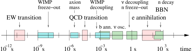
Figure 10.1. History of the first second of the Universe and the epoch of BBN. A sequence of thermodynamic transitions takes place: the electroweak transition ($\sim 10$ ps) is followed by the QCD transition ($\sim 10$ $\mu$s) and by $e^{\pm}$ annihilation ($\sim 100$ s). With respect to particles of the standard model, several important processes occur: baryons and antibaryons annihilate ($\sim 1$ ms), neutrino oscillations set in at $\sim 0.1$ s, neutrinos decouple and at the same time the neutron-to-proton ratio freezes out ($\sim 1$ s). During the epoch of BBN ($\sim 3$ min) this ratio changes slightly due to neutron decay ($\tau=886$ s). Regarding the cold dark matter candidates, WIMPs freeze out at $\sim 10$ ns and decouple kinetically at $\sim 1$ ms. The axion mass is switched on close to the QCD transition at $\sim 1$ $\mu$s.

It might be that no relics from that epoch survive and it will therefore be hard or even impossible to probe the first second directly. Nevertheless, it is mandatory to study it in detail, since this is essential to answer the following questions: (i) Why are the initial conditions for the BBN (from observations) very close to homogeneous? (ii) What is the small-scale structure of CDM and what is the implication of the CDM small-scale structure for dark matter searches? (iii) Can we exclude that CDM is baryonic? (Are quark nuggets or other QCD-relics excluded)?

Let me finally stress that this review represents my personal point of view and, there are certainly more issues than discussed here that are relevant for a complete understanding of the early Universe.

I would like to thank S. Hofmann, J. Ignatius, J. Martin, C. Schmid and P. Widerin for precious and enjoyable collaborations and I am grateful to Z. Fodor, M. Laine, S. Kraml, D. Pavón, M. Plümacher, A. Rebhan, L. Roszkowski, A. S. Sakharov, S. Sanyal, B. Tomàšik and X. Zhang for very useful comments and discussions. I thank S. Vascotto for proofreading and suggestions concerning the style.

$a$	scale factor
$B$	depending on context, baryon number or bag constant
$c_{s}$	speed of sound
$d$	distance
$f$	depending on context, frequency or volume fraction
$g$	effective number of relativistic helicity degrees of freedom
$H$	Hubble rate
$h$	depending on context, $\equiv H_{0}/(100$ km$/$s$/$Mpc$)$ or amplitude of gravitational waves
$k$	comoving wave number
$L$	lepton number
$l$	latent heat density
$M$	masses of macroscopic objects (with some noted exceptions)
$m$	particle masses
$N_{f}$	number of quark flavours
$n$	number density
$p$	pressure
$R$	radius
$s$	entropy density
$T$	temperature
$T_{*}$	transition temperature
$t$	cosmic time
$v$	velocity
$z$	redshift
$\Gamma$	interaction rate
$\epsilon$	energy density
$\zeta_{\rm visc}$	bulk viscosity
$\eta$	depending on context, $\equiv n_{\rm B}/n_{\gamma}$ or conformal time
$\eta_{\rm visc}$	shear viscosity
$\lambda$	wave length
$\mu$	chemical potential
$\rho$	mass density
$\sigma$	depending on context, surface tension or cross section
$\tau$	time scale
$\Omega$	fractional energy density
$\omega$	$\equiv\Omega h^{2}$

Table 1. List of symbols.

$0$	today	eq	matter–radiation equality
ann	annihilation	fs	free streaming
b	baryons	gw	gravitational waves
c	critical	H	typical scale set by Hubble expansion
cd	chemical decoupling	kd	kinetic decoupling
cdm	cold dark matter	m	matter $=$ baryons $+$ CDM
coll	collision	mfp	mean free path
dec	decoupling	nuc	nucleation
defl	deflagration	ph	physical
diff	diffusion	rad	radiation
dmp	damping	rms	root mean square
el	elastic	sc	supercooling

Table 2. Meaning of suffixes.

References

- [1] K. C. Roth and J. M. Bauer, Astrophys. J. 515, L57 (1999) [arXiv:astro-ph/9902295]; R. Srianand, P. Petitjean and C. Ledoux, Nature 408, 931 (2000) [arXiv:astro-ph/0012222]; J. M. LoSecco, G. J. Mathews and Yun Wang, Phys. Rev. D 64, 123002 (2001) [arXiv:astro-ph/0108260].
- [2] D. J. Fixsen et al., Astrophys. J. 473, 576 (1996) [arXiv:astro-ph/9605054]; J. C. Mather et al., Astrophys. J. 512, 511 (1999) [arXiv:astro-ph/9810373]; see also the lecture notes by G. F. Smoot, [arXiv:astro-ph/9705101].
- [3] D. N. Spergel et al., [arXiv:astro-ph/0302209].
- [4] G. F. R. Ellis and R. Maartens, [arXiv:gr-qc/0211082].
- [5] K. Hagiwara et al., Phys. Rev. D 66, 010001 (2002), http://pdg.lbl.gov/.
- [6] N. Ghodbane and H.-U. Martyn, LC Note LC-TH-2001-079 [arXiv:hep-ph/0201233]; B. C. Allanach et al., Eur. Phys. J. C 25, 113 (2002) [arXiv:hep-ph/0202233].
- [7] E. W. Kolb and M. S. Turner, The Early Universe (Addison-Wesley, Redwood City, 1990).
- [8] F. Csikor et al., Phys. Rev. Lett. 85, 932 (2000) [arXiv:hep-ph/0001087]; M. Laine and K. Rummukainen, Nucl. Phys. B 597, 23 (2001) [arXiv:hep-lat/0009025]; M. Laine, [arXiv:hep-ph/0010275].
- [9] V. Kuzmin, V. Rubakov and M. Shaposhnikov, Phys. Lett. 155B, 36 (1985).
- [10] D. Bödeker, Phys. Lett. B 426, 351 (1998) [arXiv:hep-ph/9801430].
- [11] J. A. Harvey and M. S. Turner, Phys. Rev. D 42, 3344 (1990).
- [12] A. D. Dolgov et al., Nucl. Phys. B 632, 363 (2002) [arXiv:hep-ph/0201287].
- [13] S. Hofmann, D. J. Schwarz and H. Stöcker, Phys. Rev. D 64, 083507 (2001) [arXiv:astro-ph/0104173].
- [14] E. V. Shuryak, Phys. Rep. 61, 71 (1980); D. Gross, R. Pisarski and L. Yaffe, Rev. Mod. Phys. 53, 43 (1981); F. Wilczek, Nucl. Phys. A 642, 1 (1998) [arXiv:astro-ph/9806395].
- [15] U. W. Heinz and M. Jacob, [arXiv:nucl-th/0002042]; CERN press release from 10 February 2000, http://cern.web.cern.ch/CERN/Announcements/2000/NewStateMatter/.
- [16] For some recent reviews, see U. W. Heinz, [arXiv:hep-ph/0109006]; L. McLerran, [arXiv:hep-ph/0202025].
- [17] K. Olive, Nucl. Phys. B 190, 483 (1981); E. Suhonen, Phys. Lett. 119B, 81 (1982); S. A. Bonometto and M. Sakellariadou, Astrophys. J. 282, 370 (1984).
- [18] C. J. Hogan, Phys. Lett. 133B, 172 (1983).
- [19] T. DeGrand and K. Kajantie, Phys. Lett. 147B, 273 (1984).
- [20] E. Witten, Phys. Rev. D 30, 272 (1984).
- [21] J. H. Applegate and C. J. Hogan, Phys. Rev. D 31, 3037 (1985); ibid. 34, 1938 (1986) (Erratum).
- [22] M. Gyulassy et al., Nucl. Phys. B 237, 477 (1984).
- [23] H. Kurki-Suonio, Nucl. Phys. B255, 231 (1985).
- [24] K. Kajantie and H. Kurki-Suonio, Phys. Rev. D 34, 1719 (1986).
- [25] Y. Iwasaki et al., Phys. Rev. D 46, 4657 (1992); ibid. 49, 3540 (1994); B. Grossmann and M. L. Laursen, Nucl. Phys. B 408, 637 (1993); B. Beinlich, F. Karsch and A. Peikert, Phys. Lett. B 390, 268 (1997) [arXiv:hep-lat/9608141].
- [26] G. M. Fuller, G. J. Mathews and C. R. Alcock, Phys. Rev. D 37, 1380 (1988); B. S. Meyer et al., Phys. Rev. D 43, 1079 (1991).
- [27] J. Ignatius et al., Phys. Rev. D 49, 3854 (1994) [arXiv:hep-ph/9309059]; ibid. 50, 3738 (1994) [arXiv:hep-ph/9405336].
- [28] M. B. Christiansen and J. Madsen, Phys. Rev. D 53, 5446 (1996) [arXiv:astro-ph/9602071].
- [29] J. Ignatius and D. J. Schwarz, Phys. Rev. Lett. 86, 2216 (2001) [arXiv:hep-ph/0004259].
- [30] S. Sanyal, [arXiv:hep-ph/0211208].
- [31] J. H. Applegate, C. J. Hogan and R. J. Scherrer, Phys. Rev. D 35, 1151 (1987); G. M. Fuller, G. J. Mathews and C. R. Alcock, Phys. Rev. D 37, 1380 (1988); H. Kurki-Suonio, Phys. Rev. D 37, 2104 (1988); R. A. Malaney and G. J. Mathews, Phys. Rep. 229, 145 (1993).
- [32] In-Saeng Suh and G. J. Mathews, Phys. Rev. D 58, 025001 (1998) [arXiv:astro-ph/9804090]; ibid. 58, 123002 (1998), [arXiv:astro-ph/9805179].
- [33] K. Kainulainen, H. Kurki-Suonio and E. Sihvola, Phys. Rev. D 59, 083505 (1999) [arXiv:astro-ph/9807098].
- [34] K. Jedamzik and J. B. Rehm, Phys. Rev. D 64, 023510 (2001) [arXiv:astro-ph/0101292].
- [35] R. V. Wagoner, W. A. Fowler and F. Hoyle, Astrophys. J. 148, 3 (1967); D. N. Schramm and R. V. Wagoner, Annu. Rev. Nucl. Part. Sci. 27, 37 (1977); A. M. Boesgaard and G. Steigman, Annu. Rev. Astron. Astrophys. 23, 319 (1985); T. P. Walker et al., Astrophys. J. 376, 51 (1991); M. S. Smith, L. H. Kawano and R. A. Malaney, Astrophys. J. Supp. 85, 219 (1993); C. J. Copi, D. N. Schramm and M. S. Turner, Science 267, 192 (1995) [arXiv:astro-ph/9407006]; R. E. Lopez and M. S. Turner, Phys. Rev. D 59, 103502 (1999) [arXiv:astro-ph/9807279]; D. B. Fields and S. Sakar, in [5].
- [36] J. I. Sievers et al., [arXiv:astro-ph/0205387]; A. Benoit et al., Astron. Astrophys. 399, L25 (2003) [arXiv:astro-ph/0210306]; J. H. Goldstein et al., [arXiv:astro-ph/0212517].
- [37] C. L. Bennett et al., [arXive:astro-ph/0302208].
- [38] S. Burles et al., Phys. Rev. Lett. 82, 4176 (1999) [arXiv:astro-ph/9901157]; J.M. O’Meara et al., Astrophys. J. 552 (2001) 718 [arXiv:astro-ph/0011179].
- [39] A. Coc et al., Phys. Rev. D 65, 043510 (2002) [arXiv:astro-ph/0111077].
- [40] R. H. Cyburt, B. D. Fields and K. A. Olive, [arXiv:astro-ph/0302431].
- [41] K. Jedamzik et al., Astrophys. J. 422, 423 (1994) [arXiv:astro-ph/9312066]; K. Jedamzik, [arXiv:astro-ph/9911242].
- [42] C. J. Hogan, Phys. Rev. Lett. 51, 1488 (1983).
- [43] B. Cheng and A. Olinto, Phys. Rev. D 50, 2743 (1994).
- [44] A. Zhitnitsky, [arXiv:hep-ph/0202161].
- [45] M. Alford, K. Rajagopal and F. Wilczek, Phys. Lett. B 422, 247 (1998); R. Rapp, T. Schäfer, E. V. Shuryak and M. Velkovsky, Phys. Rev. Lett. 81, 53 (1998).
- [46] R. Brandenberger, I. Halperin and A. Zhitnitsky, [arXiv:hep-ph/9808471]; [arXiv:hep-ph/9903318].
- [47] M. Crawford and D. N. Schramm, Nature 298, 538 (1982).
- [48] L. J. Hall and S. D. H. Hsu, Phys. Rev. Lett. 64, 2848 (1989); E. D. Carlson et al., Phys. Rev. Lett. 65, 2225 (1990).
- [49] K. Jedamzik, Phys. Rev. D 55, R5871 (1997) [arXiv:astro-ph/9605152]; K. Jedamzik and J. Niemayer, Phys. Rev. D 59, 124013 (1999) [arXiv:astro-ph/9901293]; Phys. Rev. D 59, 124014 (1999) [arXiv:astro-ph/9901294].
- [50] C. Schmid, D. J. Schwarz and P. Widerin, Hel. Phys. Acta 69, 198 (1996) [arXiv:astro-ph/9611186].
- [51] C. Schmid, D. J. Schwarz and P. Widerin, Phys. Rev. Lett. 78, 791 (1997) [arXiv:astro-ph/9606125].
- [52] C. Schmid, D. J. Schwarz and P. Widerin, Phys. Rev. D 59, 043517 (1999) [arXiv:astro-ph/9807257].
- [53] D. J. Schwarz, Mod. Phys. Lett. A 34, 2771 (1998) [arXiv:gr-qc/9709027].
- [54] H. Reeves, Phys. Rep. 201, 335 (1991).
- [55] S. A. Bonometto and O. Pantano, Phys. Rep. 228, 172 (1993).
- [56] R. A. Malaney and G. J. Mathews, Phys. Rep. 229, 145 (1993).
- [57] D. J. Schwarz, Nucl. Phys. A 642, 332c (1998) [arXiv:hep-ph/9807473].
- [58] B. Kämpfer, Annalen Phys. 9, 605 (2000) [arXiv:astro-ph/0004403].
- [59] P. Braun-Munzinger, D. Magestro, K. Redlich and J. Stachel, Phys. Lett. B 518, 41 (2001) [arXiv:hep-ph/0105229].
- [60] Z. Fodor and S.D. Katz, JHEP 0203, 014 (2002) [arXiv:hep-lat/0106002].
- [61] G. Boyd et al., Phys. Rev. Lett. 75, 4169 (1995) [arXiv:hep-lat/9506025]; Nucl. Phys. B469, 419 (1996) [arXiv:hep-lat/9602007].
- [62] CP-PACS Collaboration: M. Okamoto et al., Phys. Rev. D 60, 094510 (1999) [arXiv:hep-lat/9905005]; Y. Namekawa et al., Phys. Rev. D 64, 074507 (2001) [arXiv:hep-lat/0105012].
- [63] F. Karsch, Lect. Notes Phys. 583, 209 (2002) [arXiv:hep-lat/0106019]; E. Laermann and O. Philipsen, [arXiv:hep-ph/0303042].
- [64] F. Karsch, E. Laermann and A. Peikert, Nucl. Phys. B 605, 579 (2001) [arXiv:hep-lat/0012023].
- [65] CP-PACS Collaboration: A. Ali Khan et al., Phys. Rev. D 63, 034502 (2001) [arXiv:hep-lat/0008011].
- [66] CP-PACS Collaboration: A. Ali Khan et al., Phys. Rev. D 64, 074510 (2001) [arXiv:hep-lat/0103028].
- [67] A. Chodos et al., Phys. Rev. D 9, 3471 (1974); T. De Grand et al., ibid. 12, 2060 (1975); T. D. Lee, Particle Physics and Introduction to Field Theory (Harwood Academic Publishers, Chur, 1981).
- [68] E. Farhi and R. L. Jaffe, Phys. Rev. D 30, 2379 (1984).
- [69] R. Balian and C. Bloch, Ann. Phys. (N.Y.) 60, 401 (1970); ibid. 64, 27 (1971); ibid. 84, 559 (1974) (Erratum); M. S. Berger and R. L. Jaffe, Phys. Rev. C 35, 213 (1987); ibid. 44, 566 (1991) (Erratum); J. Madsen, Phys. Rev. D 50, 3328 (1994) [arXiv:hep-ph/9407314].
- [70] C. Bernard et al., Phys. Rev. D 54, 4585 (1996) [arXiv:hep-lat/9605028].
- [71] MILC Collaboration: C. W. Bernard et al., Phys. Rev. D 55, 6861 (1997) [arXiv:hep-lat/9612025].
- [72] R. Pisarski and F. Wilczek, Phys. Rev. D 29, 338 (1984); F. Wilczek, Int. J. Mod. Phys. A 7, 3911 (1992); K. Rajagopal and F. Wilczek, Nucl. Phys. B399, 395 (1993) [arXiv:hep-ph/9210253].
- [73] Y. Iwasaki et al., Z. Phys. C 71, 343 (1996) [arXiv:hep-lat/9505017]; Nucl. Phys. B (Proc. Suppl.) 47, 515 (1996) [arXiv:hep-lat/9510005].
- [74] F. R. Brown et al., Phys. Rev. Lett. 20, 2491 (1990).
- [75] J. Engels et al., Phys. Lett. B 396, 210 (1997) [arXiv:hep-lat/9612018].
- [76] M. Hackel et al., Phys. Rev. D 46, 5648 (1992).
- [77] A. Bodmer, Phys. Rev. D 4, 1601 (1971).
- [78] The E864 Collaboration: T. A. Armstrong et al., Nucl. Phys. A 625, 494 (1997) [arXiv:nucl-ex/9708001] and references therein.
- [79] C. Alcock and A. Olinto, Annu. Rev. Nucl. Part. Sci. 38, 161 (1988); Strange Quark Matter in Physics and Astrophysics, eds. J. Madsen and P. Haensel, Nucl. Phys. B (Proc. Suppl.) 24B (1991); C. Greiner and J. Schaffner-Bielich [arXiv:nucl-th/9801062]; J. Madsen, [arXiv:astro-ph/9809032].
- [80] J. Madsen and K. Riisager, Phys. Lett. B 158, 208 (1985).
- [81] K. Sumiyoshi et al., Phys. Rev. D 42, 3963 (1990).
- [82] C. Alcock and E. Farhi, Phys. Rev. D 32, 1273 (1985); J. Madsen, H. Heiselberg and K. Riisager, Phys. Rev. D 34, 2947 (1986).
- [83] K. Sumiyoshi and T. Kajino, Nucl. Phys. B (Proc. Suppl.) 24, 80 (1991); P. Bhattacharjee et al., Phys. Rev. D 48, 4630 (1993).
- [84] A. Bhattacharyya et al., Phys. Rev. D 61, 083509 (2000) [arXiv:hep-ph/9901308].
- [85] S. Banerjee et al., [arXiv:astro-ph/0211560].
- [86] MACHO Collaboration, Astrophys. J. 486, 697 (1997); EROS Collaboration, Astron. Astrophys. 324, L69 (1997).
- [87] V. Mukhanov and G. Chibisov, Pis’ma Zh. Eksp. Teor. Fiz. 33, 549 (1981) [JETP Lett. 33, 532 (1981)]; A. Starobinsky, Phys. Lett. B 117, 175 (1982); A. Guth and S.-Y. Pi, Phys. Rev. Lett. 49, 1110 (1982); S. Hawking, Phys. Lett. B 115, 295 (1982).
- [88] J. M. Bardeen, P. J. Steinhardt and M. S. Turner, Phys. Rev. D 28, 679 (1983).
- [89] J. M. Bardeen, in Cosmology and Particle Physics, ed. A. Zee (Gordon and Breach, New York, 1989).
- [90] V. F. Mukhanov, H. A. Feldman and R. H. Brandenberger, Phys. Rep. 215, 203 (1992).
- [91] J. Martin and D. J. Schwarz, Phys. Rev. D 57, 3302 (1998) [arXiv:gr-qc/9704049].
- [92] G. F. Smoot et al., Astrophys. J. 396, L1 (1992).
- [93] C. L. Bennett et al, Astrophys. J. 464, L1 (1996) [arXiv:astro-ph/9601067].
- [94] E. R. Harrison, Phys. Rev. D 1, 2726 (1970); Ya. B. Zel’dovich, Mon. Not. Roy. Astr. Soc. 160, 1P (1972).
- [95] S. Weinberg, Astrophys. J. 168, 175 (1971).
- [96] P. Sikivie, Phys. Rev. Lett. 51, 1415 (1983); C. Hagman, K. van Bibber and L. J. Rosenberg, in [5].
- [97] A. Gould, Astrophys. J. 386, L5 (1992); A. Ulmer and J. Goodman, ibid. 442, 67 (1995) [arXiv:astro-ph/9406042]; G. F. Marani et al., Astrophys. J. 512, L13 (1999) [arXiv:astro-ph/9810391].
- [98] K. Jedamzik, V. Katalinic and A. V. Olinto, Phys. Rev. D 57, 3264 (1998) [arXiv:astro-ph/9606080].
- [99] G. Sigl, A. V. Olinto and K. Jedamzik, Phys. Rev. D 55, 4582 (1997) [arXiv:astro-ph/9610201].
- [100] X. Zhang, T. Huang and R. H. Brandenberger, Phys. Rev. D 58, 027702 (1998) [arXiv:hep-ph/9711452]; R. H. Brandenberger and X. Zhang, Phys. Rev. D 59, 081301 (1999) [arXiv:hep-ph/9808306]; R. H. Brandenberger, B. Carter, A. C. Davis, Phys. Lett. B 534, 1 (2002) [arXiv:hep-ph/0202168].
- [101] M. McNeil Forbes and A. R. Zhitnitsky, Phys. Rev. Lett. 85, 5268 (2000) [arXiv:hep-ph/0004051].
- [102] A. Kosovsky, M. S. Turner and R. Watkins, Phys. Rev. Lett. 69, 2026 (1992); Phys. Rev. D 45, 4514 (1992); A. Kosovsky and M. S. Turner, Phys. Rev. D 47, 4372 (1993) [arXiv:astro-ph/9211004].
- [103] C. J. Hogan, Mon. Not. Roy. Astr. Soc. 218, 629 (1986).
- [104] M. Kamionkowski, A. Kosovsky and M. S. Turner, Phys. Rev. D 49, 2837 (1994) [arXiv:astro-ph/9310044].
- [105] B. J. Carr and J. E. Lidsey, Phys. Rev. D 48, 543 (1993); B. J. Carr, J. Gilbert and J. Lidsey, Phys. Rev. D 50, 4853 (1994) [arXiv:astro-ph/9405027].
- [106] K. Jedamzik, Phys. Rep. 307, 155 (1998) [arXiv:astro-ph/9805147].
- [107] C.Y. Cardall and G. M. Fuller, [arXiv:astro-ph/9801103].
- [108] C. Schmid and P. Widerin, [arXiv:astro-ph/9808142].
- [109] S. Weinberg, Gravitation and Cosmology (John Wiley & Sons, New York, 1972).
- [110] J.-P. Blaizot, E. Iancu and A. Rebhan, Phys. Rev. Lett. 83, 2906 (1999) [arXiv:hep-ph/9906340]; Phys. Lett. B 470, 181 (1999) [arXiv:hep-ph/9910309]; Phys. Rev. D 63, 065003 (2001) [arXiv:hep-ph/0005003].
- [111] K. Kajantie, M. Laine, K. Rummukainen and Y. Schroder, [arXiv:hep-ph/0211321].
- [112] J.-P. Blaizot and J. Y. Ollitrault, Phys. Rev. D 36, 240 (1987).
- [113] V. V. Dixit and J. Lodenquai, Phys. Lett. B 153, 240 (1985).
- [114] M. J. Fromerth and J. Rafelski, [arXiv:astro-ph/0211346].
- [115] A. A. Starobinskii, Pis’ma Zh. Eksp. Teor. Fiz. 30, 719 (1979) [JETP Lett. 30, 682 (1979)].
- [116] L. F. Abbott and D. D. Harari, Nucl. Phys. B 264, 487 (1986); B. Allen, Phys. Rev. D 37, 2078 (1988); E. D. Stewart and D. H. Lyth, Phys. Lett. B 302, 171 (1993) [arXiv:gr-qc/9302019].
- [117] V. D. Zakharov, Gravitational waves in Einstein’s theory (Halsted Press, New York, 1973).
- [118] L. M. Krauss, Nature 313, 32 (1985).
- [119] A. Vilenkin, Phys. Lett. 107B, 47 (1981); A. Vilenkin and E. P. S. Shellard, Cosmic Strings and Other Topological Defects (Cambridge University Press, Cambridge, 1994), pp. 306 f.
- [120] R. R. Caldwell and B. Allen, Phys. Rev. D 45, 3447 (1992).
- [121] D. P. Bennett, Phys. Rev. D 34, 3592 (1986); ibid. 34, 3932 (1986). R. R. Caldwell, R. A. Battye and E. P. S. Shellard, Phys. Rev. D 54, 7146 (1996) [arXiv:astro-ph/9607130].
- [122] V. M. Kaspi, J. H. Taylor and M. F. Ryba, Astrophys. J. 428, 713 (1994); S. E. Thorsett and R. J. Dewey, Phys. Rev. D 53, 3468 (1996); M. P. McHugh et al., Phys. Rev. D 54, 5993 (1996).
- [123] L. P. Csernai and J. I. Kapusta, Phys. Rev. D 46, 1379 (1992).
- [124] K. Kajantie, Phys. Lett. B 285, 331 (1992).
- [125] B. Layek, S. Sanyal and A. M. Srivastava, Phys. Rev. D 63, 083512 (2001) [arXiv:hep-ph/0101343]; [arXiv:hep-ph/0212018].
- [126] D. K. Nadezhin, I. D. Novikov and A. G. Polnarev, Astron. Zh. 55, 216 (1978) [Sov. Astron. 22, 129 (1978)]; G. V. Bicknell and R. N. Henriksen, Astrophys. J. 232, 670 (1979).
- [127] J. S. Bullock and J. R. Primack, Phys. Rev. D 55, 7423 (1997) [arXiv:astro-ph/9611106].
- [128] B. J. Carr and S. W. Hawking, Mon. Not. Roy. Astr. Soc. 168, 399 (1974).
- [129] A. Heckler and C. J. Hogan, Phys. Rev. D 47, 4256 (1993).
- [130] H. Kurki-Suonio and M. Laine, Phys. Rev. D 54, 7163 (1996) [arXiv:hep-ph/9512202], and references therein.
- [131] D. Stauffer, Phys. Rep. 54, 1 (1979).
- [132] H. Kurki-Suonio, Phys. Rev. D 37, 2104 (1988).
- [133] L. Rezzolla and J. C. Miller, Phys. Rev. D 53, 5411 (1996) [arXiv:astro-ph/9510039]; L. Rezzolla, Phys. Rev. D 54, 6072 (1996) [arXiv:hep-ph/9610225].
- [134] J. H. Applegate, C. J. Hogan, and R. J. Scherrer, Phys. Rev. D 35, 1151 (1987).
- [135] B. Banerjee and S. M. Chitre, Phys. Lett. B 258, 247 (1991); ibid. 260, 462 (1991) (Erratum).
- [136] K. Jedamzik and G. M. Fuller, Astrophys. J. 423, 33 (1994) [arXiv:astro-ph/9312063].
- [137] C. R. Alcock, G. M. Fuller and G. J. Mathews, Astrophys. J. 320, 439 (1987).
- [138] K. Jedamzik, G. M. Fuller and G. J. Mathews, Astrophys. J. 423, 50 (1994) [arXiv:astro-ph/9312065].
- [139] J. Ellis, in: Cosmology and Large Scale Structure, Les Houches, session LX, eds. R. Schaeffer et al. (Elsevier Sci., Amsterdam, 1996), pp. 825 f.
- [140] L. Covi, J. E. Kim, L. Roszkowski, Phys. Rev. Lett. 82, 4180 (1999) [arXiv:hep-ph/9905212]; L. Covi, H. B. Kim, J. E. Kim and L. Roszkowski, JHEP 0105, 033 (2001) [arXiv:hep-ph/0101009].
- [141] D. J. H. Chung, E. W. Kolb and A. Riotto, Phys. Rev. Lett. 81, 4048 (1998) [arXiv:hep-ph/9805473]; Phys. Rev. D 60, 063504 (1999) [arXiv:hep-ph/9809453].
- [142] G. Jungman, M. Kamionkowski and K. Griest, Phys. Rep. 267, 195 (1996).
- [143] For reviews, see: H. P. Nilles, Phys. Rep. 110, 1 (1984); H. E. Haber and G. L. Kane, Phys. Rep. 104, 181 (1985).
- [144] L. Roszkowski, Phys. Lett. B 262, 59 (1991); G. L. Kane, C. Kolda, L. Roszkowski and J. D. Wells, Phys. Rev. D 49, 6173 (1994) [arXiv:hep-ph/9312272]; J. Ellis et al., Phys. Rev. D 58, 095002 (1998) [arXiv:hep-ph/9801445].
- [145] J. Ellis, T. Falk, K. A. Olive and M. Schmitt, Phys. Lett. B 413, 355 (1997) [arXiv:hep-ph/9705444]; J. R. Ellis, T. Falk and K. A. Olive, Phys. Lett. B 444, 367 (1998) [arXiv:hep-ph/9810360]; L. Roszkowski, R. Ruiz de Austri and T. Nihei, JHEP 0108, 024 (2001) [arXiv:hep-ph/0106334]; A. Djouadi, M. Drees, J.L. Kneur, JHEP 0108, 055 (2001) [arXiv:hep-ph/0107316]; J. Ellis, K. A. Olive, Y. Santoso and V. C. Spanos, [hep-ph/0303043]; A. B. Lahanas and D. V. Nanopoulos, hep-ph/0303130.
- [146] K. Griest, M. Kamionkowski and M. S. Turner, Phys. Rev. D 41, 3565 (1990); K. Griest and D. Seckel, Phys. Rev. D 43, 3191 (1991); P. Gondolo and G. Gelmini, Nucl. Phys. B 360, 145 (1991); M. Drees and M.M. Nojiri, Phys. Rev. D 47, 376 (1993) [arXiv:hep-ph/9207234]; H. Baer and M. Brhlik, Phys. Rev. D 53, 597 (1996) [arXiv:hep-ph/9508321]; V. Barger and C. Kao, Phys. Rev. D 57, 3131 (1998) [arXiv:hep-ph/9704403]; A. B. Lahanas, D. V. Nanopoulos and V. C. Spanos, Phys. Lett. B 464, 213 (1999) [arXiv:hep-ph/9906394]; A. B. Lahanas, D. V. Nanopoulos and V. C. Spanos, Phys. Rev. D 62, 023515 (2000) [arXiv:hep-ph/9909497]; T. Nihei, L. Roszkowski and R. Ruiz de Austri, JHEP 0203, 031 (2002) [arXiv:hep-ph/0202009].
- [147] K. Griest, Phys. Rev. D 38, 2357 (1988); ibid. 39, 3802 (1989) (Erratum).
- [148] D. L. Tubbs and D. N. Schramm, Astrophys. J. 201, 467 (1975).
- [149] X. Chen, M. Kamionkowski and X. Zhang, Phys. Rev. D 64, 021302 (2001) [arXiv:astro-ph/0103452].
- [150] J. E. Kim, Phys. Rep. 150, 1 (1987); M. S. Turner, Phys. Rep. 197, 67 (1990); H. Murayama, in [5]; G. G. Raffelt, in [5]; C. Hagman, K. van Bibber and L. J. Rosenberg, in [5]; P. Sikivie, [arXiv:hep-ph/0211254].
- [151] A. S. Sakharov, D. D. Sokoloff and M. Yu. Khlopov, Yad. Fiz. 75, 1050 (1996) [Phys. At. Nucl. 57, 651 (1996)]; M. Yu. Khlopov, A. S. Sakharov and D. D. Sokoloff, Nucl. Phys. B (Proc. Suppl.) 72 105 (1999).
- [152] D. Gross, R. Pisarski and L. Yaffe, Rev. Mod. Phys. 53, 43 (1981); M. S. Turner, Phys. Rev. D 33, 889 (1986).
- [153] C. J. Hogan and M. J. Rees, Phys. Lett. B205, 228 (1988); E. Kolb and I. I. Tkachev, Phys. Rev. Lett. 71, 3051 (1993) [arXiv:hep-ph/9303313]; Phys. Rev. D 49, 5040 (1994) [arXiv:astro-ph/9311037]; Astrophys. J. 460, L25 (1996) [arXiv:astro-ph/9510043].
- [154] A. M. Green and A. R. Liddle, Phys. Rev. D 56, 6166 (1997) [arXiv:astro-ph/9704251].
- [155] L. Randall, M. Soljačić and A. H. Guth, Nucl. Phys. B 472, 377 (1996) [arXiv:hep-ph/9512439]; [arXiv:hep-ph/9601296]; J. Garcia-Bellido, A. Linde and D. Wands, Phys. Rev.D 54, 6040 (1996) [arXiv:astro-ph/9605094].
- [156] D. Blais, C. Kiefer and D. Polarski, Phys. Lett. B 535, 11 (2002) [arXiv:astro-ph/0203520].
- [157] P. Mészáros, Astron. Astrophys. 37, 225 (1974).
- [158] T. Padmanabhan, Structure Formation in the Universe (Cambridge University Press, Cambridge, 1993).
- [159] H. I. Kim, B.-H. Lee and C. H. Lee, Phys. Rev. D 64, 067301 (2001) [arXiv:astro-ph/9901286].
- [160] A.V. Gurevich, K.P. Zybin and V.A. Sirota, Physics-Uspekhi 40, 869 (1997).
- [161] V. Berezinsky, V. Dokuchaev and Yu. Eroshenko, [arXiv:astro-ph/0301551].
- [162] E. van Kampen, [arXiv:astro-ph/0008453].
- [163] B. Moore et al., Phys. Rev. D 64, 063508 (2001) [arXiv:astro-ph/0106271].