Projection effects on the FP thickness:

We study the contribution of projection effects to the intrinsic thickness of the Fundamental Plane (FP) of elliptical galaxies. The Monte–Carlo mapping technique between model properties and observed quantities, introduced by Bertin, Ciotti, & Del Principe (2002), is extended to oblate, two–integrals galaxy models, with non–homologous density profiles, adjustable flattening, variable amount of ordered rotational support, and for which all the relevant projected dynamical quantities can be expressed in fully analytical way. In agreement with previous works, it is found that projection effects move models not exactly parallel to the edge–on FP, by an amount that can be as large as the observed FP thickness. The statistical contribution of projection effects to the FP thickness is however marginal, and the estimated physical FP $rms$ thickness is $\simeq 90$% of the observed one (when corrected for measurement errors).

1 Introduction

In the observational three–dimensional space of central velocity dispersion $\sigma_{0}$, (circularized) effective radius $R_{\rm e}$, and mean surface brightness within the effective radius $I_{\rm e}$, early–type galaxies approximately locate on a plane, called the Fundamental Plane (hereafter FP; Dressler et al. 1987; Djorgovski & Davis 1987), and represented by the best–fit relation:

$$\log R_{\rm e}=\alpha\log\sigma_{0}+\beta\log I_{\rm e}+\gamma.$$ (1)

The coefficients $\alpha$, $\beta$, and $\gamma$ depend slightly on the considered photometric band (e.g., Pahre, de Carvalho, & Djorgovski, 1998; Scodeggio et al. 1998). By measuring $R_{\rm e}$ in kpc, $\sigma_{0}$ in km/s, and $I_{\rm e}=L/(2\pi R_{\rm e}^{2})$ in $L_{\odot}/$pc² (where $L$ is the total galaxy luminosity), reported values in the Gunn r band are $\alpha=1.24\pm 0.07$, $\beta=-0.82\pm 0.02$, $\gamma=0.182$ (Jørgensen, Franx, & Kjærgaard 1996, hereafter JFK96). One of the most striking observational properties of the FP is its small and nearly constant scatter: the distribution of $\log R_{\rm e}$ around the best–fit FP has a measured ${\it rms}$ (after correction for measurement errors, hereafter $\sigma_{\rm int}$), that corresponds to a scatter in $R_{\rm e}$ at fixed $\sigma_{0}$ and $I_{\rm e}$ ranging from 15% to 20% (see, e.g., Faber et al. 1987; JFK96).

For a stationary stellar system the scalar virial theorem can be written as

$${G\Upsilon_{*}L\over R_{\rm e}}=K_{\rm V}\sigma_{0}^{2},$$ (2)

where $\Upsilon_{*}$ is the stellar mass–to–light ratio in the photometric band used for the determination of $L$ and $R_{\rm e}$, while the coefficient $K_{\rm V}$ takes into account projection effects, the specific mass density, the stellar orbital distribution (such as velocity dispersion anisotropy and rotational support), and the effects related to the presence of dark matter. Equations (1) and (2) imply that in real galaxies, no matter how complex their structure is, $\Upsilon_{*}/K_{\rm V}$ is a well–defined function of any two of the three observables $(L,R_{\rm e},\sigma_{0})$. For example, by eliminating $\sigma_{0}$ from eqs. (1) and (2) one obtains that along the FP

$${\Upsilon_{*}\over K_{\rm V}}\propto R_{\rm e}^{(2-10\beta+\alpha)/\alpha}L^{(5\beta-\alpha)/\alpha},$$ (3)

where the dependence of the ratio $\Upsilon_{*}/K_{\rm V}$ on galaxy properties is commonly referred as the “FP tilt”. The physical content of eq. (3) is truly remarkable: all stellar systems described by eq. (2) are in virial equilibrium, but only those for which $\Upsilon_{*}/K_{\rm V}$ scales according to eq. (3) (and with the same scatter) correspond to real galaxies. In other words, eq. (3) indicates that structural/dynamical ($K_{\rm V}$) and stellar population ($\Upsilon_{*}$) properties in real galaxies are strictly connected, possibly as a consequence of their formation process: understanding the origin of the FP tilt is thus of the utmost importance for the understanding of galaxy formation.

A first possibility in this direction is to focus on the variation of a single galaxy property among the plethora in principle appearing in the quantity $\Upsilon_{*}/K_{\rm V}$, while fixing all the others to some prescribed value: we call this approach orthogonal exploration of the parameter space. For instance, one can explore the possibility that a systematic variation of $\Upsilon_{*}$ with $L$ is at the origin of the FP tilt, while considering the galaxies as strictly homologous systems (i.e., with density and dynamical structures only differing for the physical scales, and thus $K_{\rm V}=$const. See, e.g., Bender, Burstein, & Faber 1992; Renzini & Ciotti 1993; van Albada, Bertin & Stiavelli 1995, hereafter vABS; Prugniel & Simien 1996). Another possibility is to enforce a constant $\Upsilon_{*}$, and to assume that the galaxy density profiles, dark matter content and distribution, stellar orbital distribution, and so on, vary systematically with $L$ (see, e.g., Ciotti & Pellegrini 1992; Caon, Capaccioli & D’Onofrio 1993; Renzini & Ciotti 1993; Djorgovski 1995; Hjorth & Madsen 1995; Ciotti, Lanzoni & Renzini 1996, hereafter CLR; Graham & Colless 1997; Ciotti & Lanzoni 1997; Prugniel & Simien 1997).

Orthogonal explorations lead to important results, but, besides starting from a (more or less) well motivated choice of the specific parameter assumed to be responsible for the FP tilt, they also bring to a fine tuning problem: the large variation of such a parameter along the FP, necessary to reproduce the tilt, must be characterized by a small scatter of it at any fixed position on the FP in order to preserve the observed small thickness (e.g., Renzini & Ciotti 1993; CLR). Moreover, the severity of the fine tuning problem is strengthened by the unavoidable projection effects associated with the three–dimensional shape of galaxies, if they also contribute to FP thickness. Thus, the interpretation of the FP cannot be limited to the study of its tilt only, but requires to take consistently into account also its thinness.

Recently, a statistical approach to this problem, based on Monte–Carlo simulations and overcoming the intrinsic limitations of orthogonal explorations has been proposed (Bertin, Ciotti & Del Principe 2002, hereafter BCD). In this study the authors showed that, ascribing the origin of the FP tilt to the combined effect of luminosity dependent mass–to–light ratio and shape parameter $m$ in spherically symmetric and isotropic $R^{1/m}$ models (Sersic 1968), can reconcile the FP tilt with the observed large dispersion of $m$ at fixed galaxy luminosity (see Figs. 5 and 6 in CLR and Figs. 7 and 9 in BCD). Note, however, that in the BCD analysis the FP thickness is entirely produced by variations from galaxy to galaxy of their physical properties , as a consequence of the assumption of spherical symmetry. On the other hand, elliptical galaxies are in general non spherical, and the quantities entering the FP expression do depend on the observation angle: it is therefore of great interest to estimate the contribution of projection effects to the FP thickness, and to quantify its physical scatter. Few analytical works have addressed this issue in the past (e.g., Faber et al. 1987; Saglia, Bender & Dressler 1993; Jørgensen, Franx, & Kjærgaard 1993; Prugniel & Simien 1994; JFK96; vABS), their conclusions pointing in the direction of a small contribution of projection effects to the FP thickness. A different source of information on projection effects is also represented by the end–products of N–body numerical simulations (see, e.g., Pentericci, Ciotti, & Renzini 1995; Nipoti, Londrillo & Ciotti 2002ab, 2003; Gonzáles & van Albada 2002). The impression one gets from these simulations is that projection effects can be significant contributors to the FP thickness, the range spanned by the models for changing viewing angle being comparable to $\sigma_{\rm int}$ or more.

We explore this matter further, by extending the BCD approach to a class of oblate ellipsoids with non homologous density profiles, adjustable flattening and variable amount of internal velocity streaming. However, in order to maintain the dimension of the parameter space acceptable we do not take into account the presence of DM halos, and the stellar mass–to–light ratio $\Upsilon_{*}$ is assumed to be constant within each galaxy. For these models all the relevant quantities can be expressed explicitly, thus allowing for fast numerical calculation. The paper is organized as follows. In Section 2 we derive the relevant properties of the adopted models. In Section 3 we illustrate in detail a few representative cases, focusing on the effects of the various model parameters on the observational properties entering the FP relation. In Section 4 the results of the Monte–Carlo investigations are shown, and finally, in Section 5 we summarize and discuss the results. Appendix A collects the explicit formulas describing the model internal dynamics, while in Appendix B we derive the expressions for the associated projected quantities. In Appendix C the simplest model of the family (the homogeneous ellipsoid) is described in detail.

2 The models

2.1 3D quantities

In our study we use a family of oblate galaxy models with homeoidal density distribution, belonging to the so–called Ferrers ellipsoids (Ferrers 1877). The density profile is given by

$$\rho(m)=\rho_{0}\times\cases{(1-m^{2})^{n}&if $0\leq m\leq 1$,\cr 0&if $m>1$,\cr}$$ (4)

where $\rho_{0}$ is the central density, $n\geq 0$ is an integer number, and in cylindrical coordinates $(R,\varphi,z)$ the isodensity surfaces are labeled by $m^{2}\equiv R^{2}/R_{\rm t}^{2}+z^{2}/(q^{2}R_{\rm t}^{2})$. With this choice $R_{\rm t}$ is the model semi–major axis, while its flattening is given by $0<q\leq 1$. Note that these density profiles, when considered in detail, are only a rough approximation of those of real galaxies, especially for low values of $n$. However, most of the model properties that are relevant for this study show a behavior surprisingly similar to that of galaxy models with more realistic density profiles (see Sections 3). In addition the above mentioned properties can be explicitly written in analytic form, making the models suitable for Monte–Carlo simulations.

The mass within $m$ and the total mass of the models are given by

$$M(m)=\rho_{0}R_{\rm t}^{3}2\pi q{\rm B}_{3/2,n+1}(m^{2}),$$ (5)

and

$$M=\rho_{0}R_{\rm t}^{3}2\pi q{\rm B}\left({3\over 2},n+1\right),$$ (6)

respectively, where ${\rm B}_{a,b}(z)\equiv\int_{0}^{z}t^{a-1}\,(1-t)^{b-1}dt$ is the incomplete Euler Beta function, ${\rm B}(a,b)\equiv{\rm B}_{a,b}(1)=\Gamma(a)\Gamma(b)/\Gamma(a+b)$ is the complete Euler Beta function, and $\Gamma$ is the complete Euler Gamma function.

We assume that the density profiles in eq. (4) are supported by a dynamics described by a two–integrals distribution function $f=f(E,L_{z})$ (where $E$ and $L_{z}$ are the energy and the $z$ component of the angular momentum of stars). Thus, the Jeans equations reduce to

$${\partial\rho\sigma_{R}^{2}\over\partial z}=-\rho{\partial\phi\over\partial z},$$ (7)

and

$${\partial\rho\sigma_{R}^{2}\over\partial R}-{\rho(\overline{{\rm v}_{\varphi}^{2}}-\sigma_{R}^{2})\over R}=-\rho{\partial\phi\over\partial R},$$ (8)

where $\phi$ is the gravitational potential, $v_{R}=v_{z}=0$ everywhere, the off–diagonal elements of the velocity dispersion tensor vanish, and $\sigma_{R}^{2}=\sigma_{z}^{2}$ (see, e.g., Binney & Tremaine 1987, hereafter BT). The appropriate boundary conditions are $\sigma_{R}^{2}=\sigma_{z}^{2}=0$ on $m=1$ (Ciotti 2000), and so, the formal solution of eqs. (7)-(8) is:

$$\rho\sigma_{R}^{2}=\int_{z}^{z_{\rm t}}\rho{\partial\phi\over\partial z}dz,$$ (9)

where $z_{\rm t}\equiv q\sqrt{R_{\rm t}^{2}-R^{2}}$, and

$$\rho(\overline{{\rm v}_{\varphi}^{2}}-\sigma_{R}^{2})=R\left({\partial\rho\sigma_{R}^{2}\over\partial R}+\rho{\partial\phi\over\partial R}\right).$$ (10)

As it is well known, the gravitational potential of homeoidal systems can be obtained by evaluating a two–dimensional integral (see, e.g., Chandrasekhar 1969), but in general this integral cannot be expressed in terms of elementary functions. From this point of view the density profiles adopted here are a nice exception: their potential can be written explicitly (for $n$ integer) as a finite sum of integer powers of $R$ and $z$. Thus, from eqs. (9) and (10) also $\rho\sigma_{R}^{2}$ and $\rho(\overline{{\rm v}_{\varphi}^{2}}-\sigma_{R}^{2})$ can be written in the same way (their explicit expression is given in Appendix A).

To split $\overline{{\rm v}_{\varphi}^{2}}$ into streaming motion $v_{\varphi}\equiv\overline{{\rm v}}_{\varphi}$ (that for simplicity we assume nowhere negative), and azimuthal dispersion, $\sigma_{\varphi}^{2}\equiv\overline{({\rm v}_{\varphi}-v_{\varphi})^{2}}=\overline{{\rm v}_{\varphi}^{2}}-v_{\varphi}^{2}$, we adopt the Satoh (1980) $k$–decomposition:

$$v_{\varphi}^{2}=k^{2}(\overline{{\rm v}_{\varphi}^{2}}-\sigma_{R}^{2}),$$ (11)

and

$$\sigma_{\varphi}^{2}=\sigma_{R}^{2}+(1-k^{2})(\overline{{\rm v}_{\varphi}^{2}}-\sigma_{R}^{2}),$$ (12)

with $0\leq k\leq 1$. For $k=0$ no ordered motions are present, and the velocity dispersion tensor is maximally tangentially anisotropic, while for $k=1$ the velocity dispersion tensor is isotropic, and the galaxy flattening is due to azimuthal streaming velocity (the so called “isotropic rotator”). In principle, by relaxing the hypothesis of a constant $k$ and allowing for $k=k(R,z)$, even more rotationally supported models can be constructed, up to the maximum rotation case considered in Ciotti & Pellegrini (1996), where $k(R,z)$ is defined so that $\sigma_{\varphi}^{2}=0$ everywhere.

2.2 Projected quantities

To project the galaxy models on the plane of the sky (the projection plane), we employ a Cartesian coordinate system $(x\prime,y\prime,z\prime)$, with the line of sight (los) directed along the $z\prime$ axis, and with the $x\prime$ axis coincident with the $x$ axis of the natural Cartesian system introduced at the beginning of Section 2.1. The angle between $z$ and $z\prime$ is $\theta$, with $0\leq\theta\leq\pi/2$: $\theta=0$ corresponds to the face–on view of the galaxy, while $\theta=\pi/2$ to the edge–on view. With this choice, the projection plane is $(x\prime,y\prime)$, and the los direction in the natural coordinate system is given by ${\bf n}=(0,-\sin\theta,\cos\theta)$. Accordingly, the coordinates of the two Cartesian systems are related by

$$\cases{x=x\prime,\cr y=y\prime\cos\theta-z\prime\sin\theta,\cr z=y\prime\sin\theta+z\prime\cos\theta,\cr}$$ (13)

and the homeoid labeled by $m$ can be rewritten in the observer coordinate system as:

$$m^{2}=\left(\sqrt{A}\widetilde{z}\prime+{B\over\sqrt{A}}\widetilde{y}\prime\right)^{2}+\widetilde{\ell}^{2},$$ (14)

where from now on, the symbol “$\sim$” over a coordinate will indicate normalization to $R_{\rm t}$, and

$$\cases{A\equiv\sin^{2}\theta+\cos^{2}\theta/q^{2},\cr B\equiv(1/q^{2}-1)\sin\theta\cos\theta,\cr\ell^{2}\equiv x\prime^{2}+y\prime^{2}/q(\theta)^{2},\cr q(\theta)^{2}\equiv\cos^{2}\theta+q^{2}\sin^{2}\theta.\cr}$$ (15)

When integrating a model quantity along the los at given $(x\prime,y\prime)$, the limits on $z\prime$ are derived by setting $m=1$ in eq. (14)

$$\widetilde{z}\prime_{\pm}=-{B\over A}\widetilde{y}\prime\pm\sqrt{{1-\widetilde{\ell}^{2}\over A}}.$$ (16)

For examples, the surface density profile is given by

$$\Sigma_{\theta}(\ell)\equiv\int_{z\prime_{-}}^{z\prime_{+}}\rho\,dz\prime=$$

$$=\rho_{0}\,R_{\rm t}{q\over q(\theta)}{\rm B}\left({1\over 2},n+1\right)(1-\widetilde{\ell}^{2})^{n+1/2},$$ (17)

where $\rho(x\prime,y\prime,z\prime)$ is obtained by substitution eq. (14) in eq. (4). The quantity $\ell$ determines the size of the elliptic isophotes, and their (constant) apparent ellipticity is $\varepsilon=1-q(\theta)$. For a fixed $\ell$, the major and minor isophotal semiaxes are $a=\ell$ and $b=q(\theta)\ell$, and the associated circularized radius is defined by the identity $\pi R_{\ell}^{2}=\pi ab$, i.e., $R_{\ell}=\sqrt{q(\theta)}\ell$. In particular, the circularized effective radius $R_{\rm e}$ is given by

$$R_{\rm e}=\sqrt{q(\theta)}\ell_{\rm e},$$ (18)

where $\ell_{\rm e}$ is the solution of the equation $M_{\theta}(\ell_{\rm e})=M/2$, and where the projected mass within $\ell$ is

$$M_{\theta}(\ell)\equiv\int_{\ell^{{}^{\prime}}\leq\ell}\Sigma_{\theta}(\ell\prime)\,dx\prime\,dy\prime=$$

$$=\rho_{0}R_{\rm t}^{3}\,2\,\pi\,q\,{\rm B}\left({3\over 2},n+1,\right)\left[1-(1-\widetilde{\ell}^{2})^{n+3/2}\right].$$ (19)

We obtain

$$\ell_{\rm e}=\sqrt{1-2^{-1/(n+3/2)}}R_{\rm t}\equiv R_{\rm e}^{0},$$ (20)

with $R_{\rm e}^{0}$ the effective radius of the model when seen face–on (or in case of spherical symmetry). As can be easily proved, the identity $R_{\rm e}=\sqrt{q(\theta)}R_{\rm e}^{0}$ is a general property of all axisymmetric homeoidal distributions, independently of their specific density profile.

To obtain the velocity fields at $(x\prime,y\prime)$ we integrate along the los their projected component on ${\bf n}$. This is done by transforming the corresponding spatial velocity moments from cylindrical to Cartesian coordinates (see Appendix B). For example, the los component of the streaming velocity field is

$$v_{\rm n}\equiv\overline{\langle{\bf v},{\bf n}\rangle}=v_{i}n_{i},$$ (21)

where ${\langle,\rangle}$ is the standard inner product and the repeated index convention has been applied. The analogous quantity associated to the velocity dispersion tensor is

$$\sigma_{\rm n}^{2}\equiv\overline{\langle{\bf v}-\@vec{v},{\bf n}\rangle^{2}}=\sigma_{ij}n_{i}n_{j}.$$ (22)

By using the two definitions above, and eqs. (B.4)-(B.5), the expressions for $v_{\rm n}$ and $\sigma_{\rm n}^{2}$ are:

$$v_{\rm n}=-v_{\varphi}\cos\varphi\sin\theta,$$ (23)

and

$$\sigma_{\rm n}^{2}=\sigma_{R}^{2}+(1-k^{2})(\overline{{\rm v}_{\varphi}^{2}}-\sigma_{R}^{2})\cos^{2}\varphi\sin^{2}\theta,$$ (24)

where the last identity is obtained by using eq. (12). The corresponding (mass–weighted) projected fields are obtained by changing coordinates in eqs. (23) and (24), and then integrating on $z\prime$:

$$\Sigma_{\theta}(\ell)v_{\rm p}(x\prime,y\prime)\equiv\int_{z\prime_{-}}^{z\prime_{+}}\rho v_{\rm n}dz\prime,$$ (25)

$$\Sigma_{\theta}(\ell)V_{\rm p}^{2}(x\prime,y\prime)\equiv\int_{z\prime_{-}}^{z\prime_{+}}\rho v_{\rm n}^{2}dz\prime,$$ (26)

and

$$\Sigma_{\theta}(\ell)\sigma_{\rm p}^{2}(x\prime,y\prime)\equiv\int_{z\prime_{-}}^{z\prime_{+}}\rho\sigma_{\rm n}^{2}dz\prime.$$ (27)

In general $\sigma_{\rm p}^{2}$ will not coincide with the velocity dispersion we measure in observations: in fact, in presence of a non–zero projected velocity field $v_{\rm p}$, the correct definition for this quantity is

$$\Sigma_{\theta}(\ell)\sigma_{\rm los}^{2}(x\prime,y\prime)=\int_{z\prime_{-}}^{z\prime_{+}}\rho\,\,\overline{\left(\langle{\bf v},{\bf n}\rangle-v_{\rm p}\right)^{2}}dz\prime=$$

$$=\Sigma_{\theta}(\ell)\left(\sigma_{\rm p}^{2}+V_{\rm p}^{2}-v_{\rm p}^{2}\right),$$ (28)

where the last expression is derived from the identity $\overline{\langle{\bf v},{\bf n}\rangle^{2}}=\sigma_{\rm n}^{2}+v_{\rm n}^{2}$. Note that, independently of the los orientation, on the isophotal minor axis $y\prime$ (where, by definition, $\cos\varphi=0$) $v_{\rm n}$, $V_{\rm p}^{2}$, and $v_{\rm p}^{2}$ vanish, and $\sigma_{\rm n}=\sigma_{R}$: on this axis $\sigma_{\rm p}^{2}$ is the projection of $\sigma_{R}^{2}$ and $\sigma_{\rm los}^{2}=\sigma_{\rm p}^{2}$. In addition, the last identity holds everywhere when observing the galaxy face–on ($\theta=0$), or in the case $k=0$. Since the observed velocity dispersion is always measured within a given aperture, we finally integrate $\sigma_{\rm los}^{2}$ over the isophotes (even though $\sigma_{\rm los}$ in general is not constant over isophotes):

$$M_{\theta}(\ell)\sigma_{\rm los,a}^{2}(\ell)\!=\!\langle\Sigma_{\theta}\sigma_{\rm los}^{2}\rangle_{\ell}\!\equiv\!\!\!\int_{\ell^{{}^{\prime}}\leq\ell}\!\!\!\!\!\!\!\!\Sigma_{\theta}(\ell\prime)\sigma_{\rm los}^{2}(x\prime,y\prime)\,\!dx\prime\,dy\prime.$$ (29)

In Appendix B we obtain the explicit expressions for $\sigma_{\rm p}^{2}$, $V_{\rm p}^{2}$ and their aperture values. Unfortunately, $v_{\rm p}$ cannot be cast in algebraic form when $n>0$, and so we have to resort to numerical integration of eq. (25) for its evaluation; the details are given in Section 3.

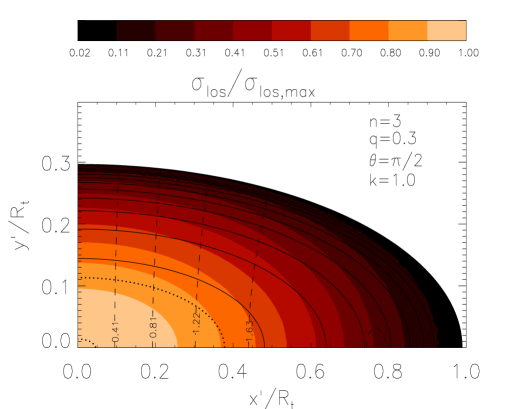
Figure 1: The projected velocity fields of the $(n=3,q=0.3,k=1)$ model, when seen edge–on ($\theta=\pi/2$). The color contour plot shows the velocity dispersion field $\sigma_{\rm los}$ normalized to its maximum value $\sigma_{\rm los,max}\simeq 0.23\,R_{\rm t}\,\sqrt{G\rho_{0}}$. Dashed lines represent the projected rotation field $v_{\rm p}/\sigma_{\rm los,max}$, with numerical values labelled in the figure. Solid lines are the surface brightness isophotes $\mu=-2.5\log\Sigma_{\theta}(\ell)$ sampled at 1 magnitude difference, while dotted lines are the isophotes corresponding to $R_{\rm e}/8$ and $R_{\rm e}$.

As a check of the exactness of the derived projected fields, we use a general consequence of the projected virial theorem (see, e.g., Ciotti 2000), i.e.

$$\langle\Sigma_{\theta}\,(\sigma_{\rm p}^{2}+V_{\rm p}^{2})\rangle_{\ell=R_{\rm t}}=2\,n_{i}n_{j}\,K_{ij}=$$

$$=-n_{1}^{2}W_{11}-n_{2}^{2}W_{22}-n_{3}^{2}W_{33},$$ (30)

where $K_{ij}$ is the kinetic energy tensor, and

$$W_{ij}=-\int\rho x_{i}{\partial\phi\over\partial x_{j}}d^{3}{\bf x},$$ (31)

are the components of the potential energy tensor. For our models, $W_{22}=W_{11}$, $n_{1}=0$, and the explicit expressions of $W_{11}$ and $W_{33}$ are given in Appendix A.

We recall that a similar approach to the one presented in this Section was adopted by vABS, who used a homeoidal, modified Jaffe density profile; in particular, they studied the projected field corresponding (in our notation) to the quantity $\sigma_{\rm los}^{2}+v_{\rm p}^{2}=\sigma_{\rm p}^{2}+V_{\rm p}^{2}$ averaged within $0.5R_{\rm e}$.

3 The model properties

To better understand the results of the Monte–Carlo simulations presented in Section 4, here we illustrate in details a few representative models, focusing on the effects of the various parameters on the projected velocity fields, and on the observational quantities entering the FP.

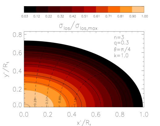
Figure 2: The fields $\sigma_{\rm los}/\sigma_{\rm los,max}$ and $v_{\rm p}/\sigma_{\rm los,max}$ of the same model in Fig. 1 when seen at $\theta=\pi/4$. In this case $\sigma_{\rm los,max}\simeq 0.24\,R_{\rm t}\,\sqrt{G\rho_{0}}$.

The projected velocity dispersion and quadratic velocity fields in eqs. (27) and (26) are evaluated by using the explicit expressions given in Appendix B. To obtain the projected field $v_{\rm p}$ in eq. (25) a numerical integration on $z\prime$ is required. For symmetry properties we restrict the computation to the first quadrant of the projection plane, that is organized with an ellipsoidal grid made of 50 uniformly spaced isophotal contours. Each contour is divided in 50 angles, while the los length $z\prime_{+}-z\prime_{-}$ (see eq. [16]) is divided in 100 elements. The computation of the projected fields on this grid, by means of a double precision Fortran90 code, requires $\simeq 20$ min on a $1.2$ GHz workstation. To check the robustness and correctness of the code, for all the explored models (many more than those presented) we have verified the projected virial theorem given in eq. (30), and we found relative errors ${\mathrel{\mathchoice{\lower 2.9pt\vbox{\halign{$\m@th\displaystyle\hfil#\hfil$\cr<\crcr\sim\crcr}}}{\lower 2.9pt\vbox{\halign{$\m@th\textstyle\hfil#\hfil$\cr<\crcr\sim\crcr}}}{\lower 2.9pt\vbox{\halign{$\m@th\scriptstyle\hfil#\hfil$\cr<\crcr\sim\crcr}}}{\lower 2.9pt\vbox{\halign{$\m@th\scriptscriptstyle\hfil#\hfil$\cr<\crcr\sim\crcr}}}}}10^{-3}$.

The illustrative cases presented here all refer to a model with $n=3$ and $q=0.3$, but their main properties apply to the whole family of models studied in this paper. Due to the constancy of the mass–to–light ratio within each model, the mass weighted and the luminosity weighted quantities are coincident.

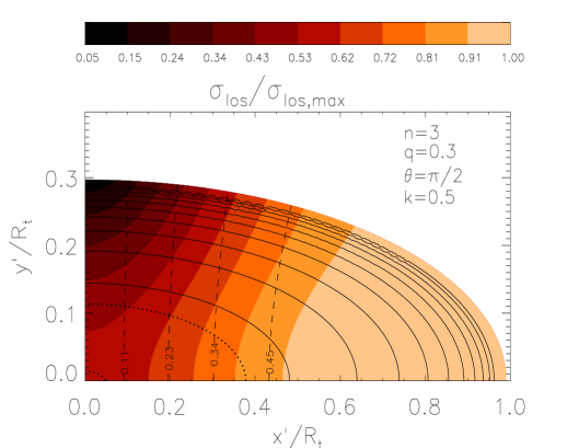
Figure 3: The fields $\sigma_{\rm los}/\sigma_{\rm los,max}$ and $v_{\rm p}/\sigma_{\rm los,max}$ of the model in Fig. 1 when seen edge–on, in case of a substantial reduction of the ordered motions ($k=0.5$). The maximum value of the velocity dispersion field is $\sigma_{\rm los,max}\simeq 0.41\,R_{\rm t}\,\sqrt{G\rho_{0}}$; all the comments in the caption of Fig. 1 apply.

Figure 1 shows the edge–on view of the two observationally accessible projected fields, $\sigma_{\rm los}$ and $v_{\rm p}$, in the isotropic rotator case. As expected, the maximum value of $\sigma_{\rm los}$ is reached at the center, while $\sigma_{\rm los}$ is not constant on isophotes. Note that inside the ellipse corresponding to a circularized radius of $R_{\rm e}/8$ (an aperture often used to correct $\sigma_{0}$ in the FP studies; e.g., JFK96), $\sigma_{\rm los}$ is constant well within 10% (in fact, better than 1%). As a consequence of the adopted decomposition of azimuthal motions and of the edge–on view of the model, the projected streaming velocity field $v_{\rm p}$ (dashed lines) is nearly vertical, its value decreases towards the center of the galaxy, and vanishes on the $y\prime$ axis. As anticipated in Section 2.1 the adopted density profiles, at variance with real galaxies, are very flat in their inner regions: this is clearly visible here, where the surface brightness $\mu=-2.5\log\Sigma_{\theta}(\ell)$ drops from the center to $R_{\rm e}$ by an amount $\Delta\mu=[(2n+1)/(2n+3)]\,2.5\,\log 2\,{\mathrel{\mathchoice{\lower 2.9pt\vbox{\halign{$\m@th\displaystyle\hfil#\hfil$\cr<\crcr\sim\crcr}}}{\lower 2.9pt\vbox{\halign{$\m@th\textstyle\hfil#\hfil$\cr<\crcr\sim\crcr}}}{\lower 2.9pt\vbox{\halign{$\m@th\scriptstyle\hfil#\hfil$\cr<\crcr\sim\crcr}}}{\lower 2.9pt\vbox{\halign{$\m@th\scriptscriptstyle\hfil#\hfil$\cr<\crcr\sim\crcr}}}}}\,1$, in contrast with the drop of more than 8 magnitudes for $R^{1/4}$ galaxies.

In Fig. 2 we show the same model seen at $\theta=\pi/4$: for obvious geometrical reasons, the lines of constant $\sigma_{\rm los}$ are now more similar to the optical isophotes. The field $\sigma_{\rm los}$ within $R_{\rm e}/8$ is still constant with very good approximation, even though $R_{\rm e}$ has increased according to eq. (18). The field $v_{\rm p}$ is deformed by projection effects, and its value, normalized to the maximum of $\sigma_{\rm los}$, is lower than in the edge–on case, as expected.

When the amount of ordered rotation is substantially reduced (for example, by assuming $k=0.5$), the resulting velocity fields are modified as shown in Fig. 3 ($\theta=\pi/2$) and in Fig. 4 ($\theta=\pi/4$). Direct comparison with Figs. 1 and 2 indicates that such a reduction of $k$ moves the maximum of $\sigma_{\rm los}$ from the center to the external regions of the model, a consequence of the increase of $\sigma_{\varphi}$ at large galactocentric distances on the equatorial plane in order to sustain the model flattening. This trend of $\sigma_{\rm los}$ is usually not observed in real galaxies, and it can be ascribed to the too “rigid” Satoh decomposition: however, $\sigma_{\rm los}$ is again nearly constant within $R_{\rm e}/8$.

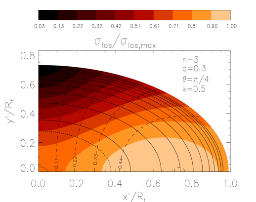
Figure 4: The fields $\sigma_{\rm los}/\sigma_{\rm los,max}$ and $v_{\rm p}/\sigma_{\rm los,max}$ of the same model in Fig. 3 when seen at $\theta=\pi/4$. In this case $\sigma_{\rm los,max}\simeq 0.31\,R_{\rm t}\,\sqrt{G\rho_{0}}$.

While we have shown here a few illustrative examples, we find that for all the models studied in detail $\sigma_{\rm los}$ stays nearly constant within $R_{\rm e}/8$. For example, for the $n=0$ model, by expanding eq. (C.11) for $\widetilde{\ell}<<1$ we obtain

$${\sigma_{\rm los,a}^{2}(\ell)\over\sigma_{\rm p}^{2}(0,0)}\sim 1+\!\left[{3(1-k^{2})\sin^{2}\theta\over 2}\!\left({w_{1}\over q^{2}w_{3}}-1\right)-1\right]{\widetilde{\ell}^{2}\over 2},$$ (32)

and so $\sigma_{\rm p}(0,0)$ and $\sigma_{\rm los,a}(R_{\rm e}/8)$ differ less than 0.1%, while for the $n=3$ models represented in Figs. 1-4 the two quantities differ less than 1%. This implies that when using apertures of the order of $R_{\rm e}/8$, the average ${\it los}$ velocity dispersion can be safely replaced by its central value, i.e., $\sigma_{\rm los,a}(R_{\rm e}/8)\simeq\sigma_{\rm los}(0,0)=\sigma_{\rm p}(0,0)$, independently of rotation and los inclination angle (note that the last identity holds exactly; see Section 2.2). These considerations are also confirmed by the cuspier models discussed in vABS.

We now describe how models “move” in the edge–on view of the FP, when changing the intrinsic (i.e., $n$, $q$, and $k$) and observational ($\theta$) parameters. In Fig. 5a we illustrate the behavior of three $n=0$ models in the ($\log R_{\rm e,FP}$, $\log R_{\rm e}$) space, where $\log R_{\rm e,FP}\equiv\alpha\log\sigma_{0}+\beta\log I_{\rm e}+\gamma$. Two models have maximum intrinsic flattening ($q=0.3$), and differ for the amount of rotation ($k=1$, and $k=0$); the third one is a rounder ($q=0.5$) isotropic rotator. Owing to the particularly simple expression of $\sigma_{\rm los,a}$ (eq. [C11]), we also investigate the effect of adopting different apertures for the estimate of $\sigma_{0}$. In all cases, varying the projection angle from 0 to $\pi/2$, makes $R_{\rm e}$ to decrease according to eq. (18), thus producing the vertical down–shift of the representative models; obviously, such a shift is smaller for the rounder galaxy. When $R_{\rm e}$ decreases $I_{\rm e}$ increases, and galaxy models move along straight lines of constant inclination with respect to the edge–on FP, independently of their specific density distribution (see comments below eq. [20]), and provided that $\sigma_{0}$ is only weakly dependent on the los inclination. We find that even when $\sigma_{0}$ is measured within apertures of up to the order of $R_{\rm e}$, the effect on the model displacement in the FP is marginal, independently of the viewing angle and the amount of rotational support. The only relevant case is when the total aperture is considered (circles) and the galaxy flattening is supported by the azimuthal velocity dispersion (these results can be qualitatively interpreted by using eq. [C.11] with $\widetilde{\ell}=1$). In Fig. 5b, the effect of the viewing angle for different values of the shape parameter $n$ is illustrated. At variance with Fig. 5a, all models have the same flattening ($q=0.3$), mass, mass–to–light ratio, and truncation radius. The amount of projection effects is quantitatively similar for different values of $n$, being mainly due to the dependence of $R_{\rm e}$ on the viewing angle. In summary, since in all cases the directions along which models move are not parallel to the FP best fit line, projection effects do contribute to the observed FP scatter, with effects ${\mathrel{\mathchoice{\lower 2.9pt\vbox{\halign{$\m@th\displaystyle\hfil#\hfil$\cr<\crcr\sim\crcr}}}{\lower 2.9pt\vbox{\halign{$\m@th\textstyle\hfil#\hfil$\cr<\crcr\sim\crcr}}}{\lower 2.9pt\vbox{\halign{$\m@th\scriptstyle\hfil#\hfil$\cr<\crcr\sim\crcr}}}{\lower 2.9pt\vbox{\halign{$\m@th\scriptscriptstyle\hfil#\hfil$\cr<\crcr\sim\crcr}}}}}2\sigma_{\rm int}$.

Interestingly, from Fig. 5b it is also evident that the trend of $n$ along the FP is in agreement with what found observationally when galaxy light profiles are fitted with the $R^{1/m}$ models (e.g., Caon et al. 1993; CLR; Graham & Colless 1997; Prugniel & Simiens 1997; Ciotti & Lanzoni 1997; BCD): in fact, in this latter class, an increase of $m$ corresponds to the galaxy density profile being radially flatter in the external regions, as Ferrers models behave for decreasing $n$. However, the amount of this effect in Ferrers density profiles is substantially smaller. This can be estimated by considering the behavior of $K_{\rm V}=GM/R_{\rm e}\sigma_{\rm p}^{2}(0,0)$: in the spherical limit, $4.93\,{\mathrel{\mathchoice{\lower 2.9pt\vbox{\halign{$\m@th\displaystyle\hfil#\hfil$\cr<\crcr\sim\crcr}}}{\lower 2.9pt\vbox{\halign{$\m@th\textstyle\hfil#\hfil$\cr<\crcr\sim\crcr}}}{\lower 2.9pt\vbox{\halign{$\m@th\scriptstyle\hfil#\hfil$\cr<\crcr\sim\crcr}}}{\lower 2.9pt\vbox{\halign{$\m@th\scriptscriptstyle\hfil#\hfil$\cr<\crcr\sim\crcr}}}}}\,K_{\rm V}(n)\,{\mathrel{\mathchoice{\lower 2.9pt\vbox{\halign{$\m@th\displaystyle\hfil#\hfil$\cr<\crcr\sim\crcr}}}{\lower 2.9pt\vbox{\halign{$\m@th\textstyle\hfil#\hfil$\cr<\crcr\sim\crcr}}}{\lower 2.9pt\vbox{\halign{$\m@th\scriptstyle\hfil#\hfil$\cr<\crcr\sim\crcr}}}{\lower 2.9pt\vbox{\halign{$\m@th\scriptscriptstyle\hfil#\hfil$\cr<\crcr\sim\crcr}}}}}\,6$ for $0\leq n\leq 10$, to be compared with the range $7.96\,{\mathrel{\mathchoice{\lower 2.9pt\vbox{\halign{$\m@th\displaystyle\hfil#\hfil$\cr>\crcr\sim\crcr}}}{\lower 2.9pt\vbox{\halign{$\m@th\textstyle\hfil#\hfil$\cr>\crcr\sim\crcr}}}{\lower 2.9pt\vbox{\halign{$\m@th\scriptstyle\hfil#\hfil$\cr>\crcr\sim\crcr}}}{\lower 2.9pt\vbox{\halign{$\m@th\scriptscriptstyle\hfil#\hfil$\cr>\crcr\sim\crcr}}}}}\,K_{\rm V}(m)\,{\mathrel{\mathchoice{\lower 2.9pt\vbox{\halign{$\m@th\displaystyle\hfil#\hfil$\cr>\crcr\sim\crcr}}}{\lower 2.9pt\vbox{\halign{$\m@th\textstyle\hfil#\hfil$\cr>\crcr\sim\crcr}}}{\lower 2.9pt\vbox{\halign{$\m@th\scriptstyle\hfil#\hfil$\cr>\crcr\sim\crcr}}}{\lower 2.9pt\vbox{\halign{$\m@th\scriptscriptstyle\hfil#\hfil$\cr>\crcr\sim\crcr}}}}}\,1.75$ for $1\leq m\leq 10$ in case of $R^{1/m}$ models (BCD). Thus, while structural non–homology alone, with constant $\Upsilon_{*}$, is sufficient to reproduce the whole tilt of the FP in the case of the $R^{1/m}$ models (CLR; Ciotti & Lanzoni 1997; BCD), this is not true for the Ferrers ellipsoids. Also note that, at least in the spherical limit, the values of $K_{\rm V}(n)$ are within the range spanned by the virial coefficient in the case of the $R^{1/m}$ models. In particular, they are close to the value of 4.65 that characterizes the de Vaucouleurs profile $R^{1/4}$. Since $K_{\rm V}$ is the only model-dependent property that explicitly enters the FP relation (through eq. [3]), this ensures that the class of models we are using is suitable for our investigation. The behavior of $K_{\rm V}(n)$ for different flattenings and viewing angles is summarized in Table 1.

Figure 5: Panel a: effects of los direction and spectroscopic aperture on three $n=0$ models, arbitrarily placed on the edge-on FP (solid line), as a function of flattening ($q$) and amount of ordered rotation ($k$). Dotted lines mark $\sigma_{\rm int}$. In each model, the three aperture radii are $R_{\rm e}/8$ (squares), $R_{\rm e}$ (triangles), whole aperture (circles), and for each aperture radius, the three points at decreasing $y$-axis correspond to $\theta=0,\,\pi/4,\,\pi/2$. Panel b: effects of los direction and density profile on the position of the models along the edge–on FP, when $\sigma_{0}=\sigma_{\rm p}(0,0)$. As in panel a, $\theta$ increases along the arrows.

Table 1: The quantity $K_{\rm V}$ for Ferrers ellipsoids as a function of $n$, $q$, and viewing angle $\theta$, when $\sigma_{0}=\sigma_{\rm p}(0,0)$.

$K_{\rm V}$	$q=1$	$q=0.3$	$q=0.3$
		$\theta=0$	$\theta=\pi/2$
$n=0$	4.93	8.29	15.13
$n=3$	5.78	8.61	17.36
$n=6$	5.92	8.68	17.72
$n=10$	6.00	8.71	17.89

Figure 6: Accepted models (dots) selected according to eq. (34) and $\sigma_{\rm inp}=0.054$, plotted in the edge-on (Panel a), and face-on (Panel b) views of the FP. For models in Panel a, $\sigma_{\rm int}=0.057$. Solid triangles are the Coma cluster galaxies in Gunn r (from JFK96). Panel c: the edge-on FP for the models selected in the “zero–thickness” approximation. Solid and dashed lines in Panels a and c represent eq. (1) and its intrinsic scatter, respectively. The dotted line in Panel b marks the “zone of exclusion” (JFK96).

4 Simulations and results

4.1 The numerical procedure

In this Section we extend the statistical approach presented in BCD, and we determine the most general manifold (in the parameter space) defined by the models that lie on the observed FP. In practice, for each seven–dimensional point $(n,\Upsilon_{*},L,R_{\rm t},q,k,\theta)$ in the model space, we determine $R_{\rm e}$, $I_{\rm e}$, and $\sigma_{0}$. Then, we check if the model “belongs” to the FP. The observational FP that we take as a reference is the one obtained by JFK96 for the Coma cluster galaxies in Gunn r (eq. [1]). For its intrinsic scatter we adopt the value $\sigma_{\rm int}=0.057$, as quoted by JFK96 for the galaxies with $\sigma_{0}\geq 100$ km/s.

The domains of model parameters considered in the simulations are the following: $0\leq n\leq 6$, $1\leq\Upsilon_{*}\leq 10$ (different from galaxy to galaxy, but constant within each model), $2.7\leq L\leq 50$ (in $10^{10}\,L_{\odot}$, the same range of values spanned by the JFK96 Coma cluster galaxies), $1\leq R_{\rm t}\leq 200$ (in kpc), $0.3\leq q\leq 1$, and $0\leq\theta\leq\pi/2$. The values of $n$ and $\Upsilon_{*}$ are randomly extracted from uniform distributions, while power-law distributions $p(L)\propto L^{-1}$ and $p(R_{\rm t})\propto R_{\rm t}^{-1.5}$ have been used to extract $L$ and $R_{\rm t}$ by means of the von Neuman rejection technique. The assumption of strongly non uniform input distributions for $L$ and $R_{\rm t}$ was necessary in order to end (after the FP selection) with galaxy models having a luminosity function and a distribution of effective radii in agreement with those observed (see Sect. 4.3). For the extraction of the flattening $q$ a fit to the observed distribution of intrinsic ellipticity (as derived for a population of oblate spheroids by Binney & de Vaucouleurs, 1981)

$$p(q)\simeq{0.6(q+0.055)(q^{2}-1.07q+0.377)\over q^{2}-1.197q+0.372},$$ (33)

has been used. Even though the assumption of a population made of oblate spheroids only is not fully consistent with observations (see, e.g., Binney & Merrifield 1998), it is acceptable for our investigation, and it is also consistent with the geometry of the adopted models. Concerning the estimate of the model central velocity dispersion, we recall that the way how models move along the FP is almost the same when using apertures of $R_{\rm e}/8$ or $R_{\rm e}$, and so, according to the results of Section 3, we assume $\sigma_{0}=\sigma_{\rm p}(0,0)$. In such a way the dimensionality of the parameter space is reduced by excluding $k$ from the analysis. Finally, to sample the effect of the los inclination, we compute the projections of each model along 11 viewing angles equally spaced in $0\leq\cos\theta\leq 1$.

For each projection angle we first check whether $R_{\rm e}$ and $\sigma_{0}$ are within the ranges $1\leq R_{\rm e}/{\rm kpc}\leq 20$ and $100\leq\sigma_{0}/({\rm km/s)}\leq 350$; if not, the model is discarded as unrealistic, otherwise we construct the angle average quantities $\langle\log R_{\rm e}\rangle$, $\langle\log\sigma_{0}\rangle$, $\langle\log I_{\rm e}\rangle$, and $\langle\log R_{\rm e,FP}\rangle=\alpha\,\langle\log\sigma_{0}\rangle+\beta\,\langle\log I_{\rm e}\rangle+\gamma$, we calculate the quantity $\langle\Delta{\rm FP}\rangle\equiv\langle\log R_{\rm e}\rangle-\langle\log R_{\rm e,FP}\rangle$, and we apply the following criteria to check whether this candidate model “belongs” or not to the FP. Since the FP residuals are consistent with being distributed as a Gaussian (JFK96), we require that, according to the von Neuman rejection technique, the angle average model is extracted from the distribution

$$p(\langle\Delta{\rm FP}\rangle)\propto\exp({-\langle\Delta{\rm FP}\rangle^{2}/2\,\sigma_{\rm inp}^{2}}),$$ (34)

where $\sigma_{\rm inp}$ is an input parameter. We finally accept the model if it also belongs to the face-on FP, i.e., if it satisfies $0.54\,x+y{\mathrel{\mathchoice{\lower 2.9pt\vbox{\halign{$\m@th\displaystyle\hfil#\hfil$\cr<\crcr\sim\crcr}}}{\lower 2.9pt\vbox{\halign{$\m@th\textstyle\hfil#\hfil$\cr<\crcr\sim\crcr}}}{\lower 2.9pt\vbox{\halign{$\m@th\scriptstyle\hfil#\hfil$\cr<\crcr\sim\crcr}}}{\lower 2.9pt\vbox{\halign{$\m@th\scriptscriptstyle\hfil#\hfil$\cr<\crcr\sim\crcr}}}}}4.2$, with $2.66\,x\equiv 2.21\langle\log R_{\rm e}\rangle-0.82\langle\log I_{\rm e}\rangle+1.24\langle\log\sigma_{0}\rangle$, and $1.49\,y\equiv 1.24\langle\log I_{\rm e}\rangle+0.82\langle\log\sigma_{0}\rangle$ (JFK96).

The end product of a complete run is the data sample composed by the 11 projections of each accepted model. For this sample, in the $(\log R_{\rm e,FP},\log R_{\rm e})$ space we estimate both the linear best–fit and the ${\it rms}$ of the residuals around the best fit line, ${\it rms}(\Delta{\rm FP})$. The procedure is repeated by changing the input parameters $\sigma_{\rm inp}$ until ${\it rms}(\Delta{\rm FP})=0.057$. The physical thickness of the FP is then evaluated as ${\it rms}(\langle\Delta{\rm FP}\rangle)$, and the contribution of projection effects is estimated as $\sigma_{\rm proj}=\sqrt{{\it rms}(\Delta{\rm FP})^{2}-{\it rms}(\langle\Delta{\rm FP}\rangle)^{2}}$.

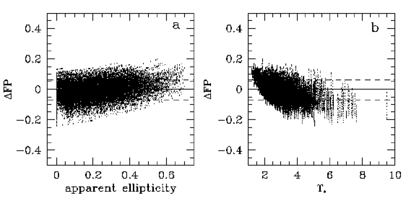
Figure 7: Distribution of the residuals about the FP as a function of apparent ellipticity (panel a) and mass–to–light ratio (panel b), for models reproducing the observed FP. Points within the dashed lines correspond to models with $|R_{\rm e}/R_{\rm e,FP}-1|{\mathrel{\mathchoice{\lower 2.9pt\vbox{\halign{$\m@th\displaystyle\hfil#\hfil$\cr<\crcr\sim\crcr}}}{\lower 2.9pt\vbox{\halign{$\m@th\textstyle\hfil#\hfil$\cr<\crcr\sim\crcr}}}{\lower 2.9pt\vbox{\halign{$\m@th\scriptstyle\hfil#\hfil$\cr<\crcr\sim\crcr}}}{\lower 2.9pt\vbox{\halign{$\m@th\scriptscriptstyle\hfil#\hfil$\cr<\crcr\sim\crcr}}}}}0.15$.

Note that in this approach, due to the high dimensionality of the parameter space, to the thinness of the FP, and to the von Neuman rejections on $L$, $R_{\rm t}$, $q$, and $\langle\Delta{\rm FP}\rangle$, we usually need to calculate several hundreds thousand projected models for each choice of $\sigma_{\rm inp}$. This is feasible with the adopted class of models, because $R_{\rm e}$ and $\sigma_{0}$ can be expressed in a fully analytical way.

4.2 Projection effects on the FP thickness

Following the procedure described above, we find that for $\sigma_{\rm inp}\simeq 0.054$ the sample of accepted models defines a synthetic FP that matches very well the observed one, both in the edge-on (Fig. 6a) and in the face-on (Fig. 6b) views. The model FP is characterized (by construction) by ${\it rms}(\Delta{\rm FP})=\sigma_{\rm int}$, while its physical thickness is ${\it rms}(\langle\Delta{\rm FP}\rangle)\sim 0.052=0.91\sigma_{\rm int}$. It follows that $\sigma_{\rm proj}\sim 0.41\sigma_{\rm int}$. In this simulation, the fraction of accepted models is $\sim 2.2\%$.

Another possibility to estimate the contribution of projection effects to the FP thickness is that of selecting the angle averaged models from what we call the “zero–thickness” FP: in practice, we adopted $\sigma_{\rm inp}=0.001$ in eq. (34), so that the dispersion produced by the accepted models when seen from the 11 different los is entirely due to projection. Note how, in agreement with the results shown in Fig. 5, the final data set nicely fills the $1\sigma$ strip in Fig. 6c. In these zero–thickness realizations, the fraction of accepted model is $\sim 0.4\%$, and ${\it rms}(\Delta{\rm FP})\simeq 0.45\,\sigma_{\rm int}$. Accordingly, we quantify the physical FP scatter as $\sigma_{\rm phys}=\sqrt{\sigma_{\rm int}^{2}-\sigma_{\rm proj}^{2}}\simeq 0.89\sigma_{\rm int}$.

As a test of the robustness of the above estimates we also explored the case in which the distribution of $\Delta{\rm FP}$ is a step function, i.e., instead of using eq. (34), we accept the model if

$$\delta\equiv|10^{\langle\Delta{\rm FP}\rangle}-1|\leq\delta_{\rm inp},$$ (35)

and we chose $\delta_{\rm inp}$ so that ${\it rms}(\Delta{\rm FP})$ of the selected models equals $\sigma_{\rm int}$: the resulting values for $\sigma_{\rm phys}$ and $\sigma_{\rm proj}$ are in perfect agreement with those obtained with the previous approach.

For the whole sample of models that reproduces the observed FP no systematic trends with the FP residuals are shown by $n$, $q$, $R_{\rm e}$, $L$, $\sigma_{0}$, while we find marginal correlations between the apparent ellipticity $\epsilon=1-q(\theta)$ and the mass-to-light ratio $\Upsilon_{*}$, and $\Delta{\rm FP}$. In agreement with the analysis of JFK96 (cfr. Fig.8a therein) and Saglia et al. (1993), flatter galaxies in projection are preferentially characterized by positive residuals (Fig. 7a), while $\Delta{\rm FP}$ decreases from positive to negative values for increasing $\Upsilon_{*}$ (Fig. 7b).

4.3 The FP tilt

We now address the issue of the FP tilt, and compare the properties of the models that reproduce the observed FP against the available observational counterparts.

Figure 8: Histograms of the properties of the models reproducing the observed FP (solid lines). Dotted histograms in panels a, b, c correspond to the observational data for the Coma cluster in Gunn r (from JFK96). The dotted line in panel d represents the input distribution of $q$, as given in eq. (33).

In Fig. 8 the distributions of the model properties are shown with solid lines, while those of the adopted observational sample are represented with dotted lines. From Figs. 8 it is apparent how the FP selection modifies the input power-law distributions of $L$ and $R_{\rm t}$ into distributions that match remarkably well the observed ones for $L$ and $R_{\rm e}$. In particular, the result should be contrasted with the one (not shown here) obtained when extracting $L$ and $R_{\rm t}$ from uniform distributions: in that case, $\log L$ and $R_{\rm e}$ peak at $\sim$1.1 and $\sim$14, respectively. An interesting case is presented by the flattening $q$: in Fig. 8d it is apparent how the input distribution (dotted curve) is not modified by the FP selection. Also the effect on the shape parameter $n$ is not very strong, even if the FP seems to be marginally selective against the lowest and the highest values of $n$ (Fig. 8e). On the contrary, the effect on the mass-to-light ratio is remarkable: its input uniform distribution has been substantially altered towards small values by the FP selection (Fig. 8f). Note the peak around $\Upsilon_{*}\simeq 3$, a value in good agreement with the commonly accepted stellar mass–to–light ratios in elliptical galaxies in the Gunn r band.

Figure 9: Distribution along the FP of luminosity and mass–to–light ratio of the models that reproduce the observed FP (dots). Solid triangles correspond to the observational data for the Coma cluster in Gunn r (from JFK96).

We now describe how the model properties vary along the FP. While $n$ and $q$ do not show any particular trend or segregation, $L$ and $\Upsilon_{*}$ are found to systematically increase with $R_{\rm e,FP}$ (Fig. 9). In both cases, the scatter is large, but almost constant for fixed $R_{\rm e,FP}$. As shown in Fig. 9a, not only the trend of $L$ with $R_{\rm e,FP}$, but also the overall region populated by the models in this space, correspond remarkably well to those found in the observations.

The distributions of $L$ and $\Upsilon_{*}$ along the FP translate in a well defined mutual dependence of these model properties, as illustrated in Fig. 10 (small dots). Also in this case the agreement with the estimates from the observational data is remarkable (cfr. Fig.3a in JFK96). The large scatter in $\Upsilon_{*}$ at fixed $L$ is by construction consistent with the small thickness of the FP: apparently, other model properties vary within the sample of accepted models so that their combined effect is to maintain the FP thin. A clearer view of the situation can be obtained by considering only galaxy models lying on the idealized zero–thickness FP (open circles): the relation between $\Upsilon_{*}$ and $L$ is better defined now, even though the scatter in $\Upsilon_{*}$ at fixed $L$ is still significant. In case of an orthogonal exploration based on a systematic trend of $\Upsilon_{*}$ with galaxy luminosity, the set of models would be just a 1–dimensional line in Fig. 10 (cfr. to Fig. 6 in BCD). Here, such a case can be mimicked by restricting further to a sub–sample of models characterized by a small range of flattenings (for example, $0.9\leq q\leq 1$, filled triangles in Fig. 10). For this latter data set, the strict correlation $\Upsilon_{*}\propto L^{0.3}$ is obtained, as predicted by eq. (3) with $K_{\rm V}\sim\,$const.

We recall that in this class of models $n$ has only a minor effect in determining $\sigma_{0}$ (at variance with the shape parameter in the case of $R^{1/m}$ models). However, the behavior of the density profiles and $L$ is qualitatively the same in the two families, as discussed at the end of Section 3. In fact, when limiting to Ferrers ellipsoids with constant $\Upsilon_{*}$ and $q$, a correlation between the shape parameter and the luminosity appears, with $n$ decreasing for increasing $L$.

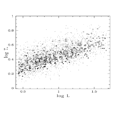
Figure 10: $\Upsilon_{*}$ vs. $L$ for the models that reproduce the observed FP (small dots). Circles correspond to models belonging to the zero–thickness FP, while black filled triangles are their sub–sample in which $0.9\leq q\leq 1$.

5 Discussion and Conclusions

In this paper we have explored the importance of projection effects on the FP thickness. We extended the statistical approach introduced by BCD to a class of oblate galaxy models, with variable density profile, flattening, amount of rotation, and fully analytical spatial and projected dynamical properties. In particular, after generating galaxy models corresponding to random choices of the model parameters, we retained only those defining a FP with the same tilt and thickness as the observed one. With this approach not only we quantified the importance of projection effects on the observed FP thickness (thus also determining the “physical” FP scatter associated to the dispersion in the galaxy internal properties), but we also studied in a consistent way the possible origins of the FP tilt. Such a framework represents a valuable alternative to the somewhat arbitrary orthogonal explorations, where the property responsible for the FP tilt is selected a priori, and a fine tuning problem for the selected parameter is unavoidable. In the present approach instead, we find that model properties can vary significantly from galaxy to galaxy, while preserving the observed FP thinness (a result in agreement with what found by BCD). Of course, we stress again that (at a deeper level) the very existence of the FP with such a small scatter is a fine tuning case, in the sense that stellar population ($\Upsilon_{*}$) and structural and dynamical properties ($K_{\rm V}$) are tightly correlated, as described by eq. (3). The reason for that can only be found in a comprehensive theory of galaxy formation and evolution.

The main results of the present work can be summarized as follow:

• For the adopted class of models the contribution of ordered streaming motions to the observed velocity dispersion is negligible when small/medium apertures (${\mathrel{\mathchoice{\lower 2.9pt\vbox{\halign{$\m@th\displaystyle\hfil#\hfil$\cr<\crcr\sim\crcr}}}{\lower 2.9pt\vbox{\halign{$\m@th\textstyle\hfil#\hfil$\cr<\crcr\sim\crcr}}}{\lower 2.9pt\vbox{\halign{$\m@th\scriptstyle\hfil#\hfil$\cr<\crcr\sim\crcr}}}{\lower 2.9pt\vbox{\halign{$\m@th\scriptscriptstyle\hfil#\hfil$\cr<\crcr\sim\crcr}}}}}\,R_{\rm e}$) are used for the spectroscopic observations. This implies that a systematic decrease of rotational support with increasing luminosity is not at the origin of the FP tilt of elliptical galaxies. However, the contribution of rotation can be non negligible when using larger apertures, and this must be taken properly into account when studying the FP at high redshift.

• When observed from different los inclinations models move along a direction that is not exactly parallel to the best fit line of the edge–on FP, thus confirming that projection effects do contribute to the observed FP scatter. The amount of such a shift depends mainly on the intrinsic flattening of the models (being larger for more flattened systems) and, to a minor extent, on the adopted aperture used for the determination of $\sigma_{0}$.

• The estimated contribution of projection effects to the observed dispersion of $\log R_{\rm e}$ around the FP is $\sim 0.4\,\sigma_{\rm int}$, while the FP physical scatter (as determined by variations of the physical properties from galaxy to galaxy), is $\sim 0.9\,\sigma_{\rm int}$. It follows that, when studying the correlations between galaxy properties required to reproduce the FP tilt and thickness, spherical models are an acceptable approximation.

• Weak correlations of the FP residuals with galaxy mass–to–light ratio and apparent ellipticity are found. The latter is in good agreement with the results of JFK96 and Saglia et al. (1993).

• For the models that reproduce the observed FP, a very good agreement between their properties ($L$, $R_{\rm e}$, $\sigma_{0}$, and $q$) and the observational data if found. Also the trend of $\Upsilon_{*}$ with $L$ corresponds very well to the one estimated from the observations. In order to get these results, it has been crucial to extract the models from steep power-law distributions of $L$ and $R_{\rm t}$, while uniform distributions in input produce an excess of models with bright luminosities and large effective radii. While the conclusions about the contribution of projection effects to the physical FP thickness would remain unchanged, it is still unclear why the requirement that models belong to the FP is so selective against low $L$ and $R_{\rm e}$.

• For what concerns the FP tilt, $L$ and $\Upsilon_{*}$ of the accepted models appear to systematically increase with $R_{\rm e,FP}$. The corresponding increase of $\Upsilon_{*}$ with $L$ is also well defined and in very good agreement with the observational estimates. In addition, in the ($\Upsilon_{*},\,L$) plane, the models appear to be segregated in terms of the flattening: at any fixed $L$, systems with low $\Upsilon_{*}$ are preferentially rounder than those with high $\Upsilon_{*}$.

• The ranges of variation of the shape parameter $n$, flattening, and mass–to–light ratio for models of given luminosity can be very large, although consistent (by construction) with a thin FP. This naturally solves the fine tuning problem met by the “orthogonal exploration” approach, and it provides better agreement with observational data. In practice, model parameters mutually combine in such a way that a large dispersion of galaxy properties is allowed at any fixed location of the FP, while preserving its thinness.

For simplicity we have used, as a guiding tool for the present investigation, simple one–component, two–integrals oblate galaxy models. The study would be best carried out with other families of models, better justified from the observational and physical point of view, but for the present purposes the simple models used provide an adequate demonstration. In fact, although the density distributions adopted here are not a good representation of real elliptical galaxies, the conclusions obtained about the projection effects on the FP can be considered robust. In fact, it is also reassuring that the displacements in the FP space of our models due to a change in the los direction agree both qualitatively and quantitatively with the analogous results obtained from the end–products of N–body simulations. This is because the way $R_{\rm e}$ (and thus $I_{\rm e}$) depends on the viewing angle is the same for all homeoidally stratified density distributions. A substantial improvement of the present exploration, assuming more realistic density profiles, would require much more time expensive simulations, since numerical calculation of the projected velocity dispersion would be necessary.

Appendix A 3D quantities

A.1 Potential expansion and gravitational energy

The general quadrature formula for the potential at internal points of heterogeneous homeoidal distributions, can be rewritten in the specific case of oblate Ferrers ellipsoids as

$$\phi(R,z)=-\pi GR_{\rm t}^{3}q\int_{0}^{\infty}{\Delta\Psi(\tau)\over\Delta(\tau)}d\tau,$$ (36)

where

$$\Delta\Psi(\tau)\equiv 2\int_{m(\tau)}^{\infty}\rho(t)tdt=\rho_{0}{[1-m^{2}(\tau)]^{n+1}\over n+1},$$ (37)

$$m^{2}(\tau)\equiv{R^{2}\over R_{\rm t}^{2}+\tau}+{z^{2}\over q^{2}R_{\rm t}^{2}+\tau},$$ (38)

and

$$\Delta(\tau)\equiv(R_{\rm t}^{2}+\tau)\sqrt{q^{2}R_{\rm t}^{2}+\tau}.$$ (39)

After a double expansion of identity (A.2) a cumbersome but trivial algebra shows that eq. (A.1) can be written as

$$\phi(R,z)=-\pi G\rho_{0}R_{\rm t}^{2}\sum_{i=0}^{n+1}\sum_{j=0}^{i}\phi_{nij}(q)\widetilde{R}^{2(i-j)}\widetilde{z}^{2j},$$ (40)

where $\widetilde{R}\equiv R/R_{\rm t}$, $\widetilde{z}\equiv z/R_{\rm t}$,

$$\phi_{nij}(q)\equiv{q(-1)^{i}\over(n+1)(i+1/2)}{n+1\choose i}{i\choose j}\,$$

$$\leavevmode\nobreak\ \leavevmode\nobreak\ \leavevmode\nobreak\ \leavevmode\nobreak\ \leavevmode\nobreak\ \leavevmode\nobreak\ \leavevmode\nobreak\ \leavevmode\nobreak\ \leavevmode\nobreak\ \leavevmode\nobreak\ \leavevmode\nobreak\ \leavevmode\nobreak\ \leavevmode\nobreak\ \leavevmode\nobreak\ {}_{2}{\rm F}_{1}\left(j+{1\over 2},i+{1\over 2},i+{3\over 2};1-q^{2}\right),$$ (41)

and ${}_{2}{\rm F}_{1}$ is the standard hypergeometrical function defined by

$${}_{2}{\rm F}_{1}(a,b,c;z)\!=\!{\Gamma(c)\over\Gamma(b)\Gamma(c-b)}\!\int_{0}^{1}\!\!t^{b-1}(1-t)^{c-b-1}(1-zt)^{-a}dt,$$ (42)

with $c>b>0$ and $\mid z\mid<1$. Note that ${}_{2}{\rm F}_{1}(a,b,c;0)=0$ and that for $i$ and $j$ integers, ${}_{2}{\rm F}_{1}$ in eq. (A.6) reduces to a combination of elementary functions.

The components of the gravitational energy tensor used at the end of Subsection 2.2 can be evaluated from the useful identities

$$W_{ij}=-GR_{\rm t}^{4}\pi^{2}qa^{2}_{i}w_{i}\delta_{ij}\int_{0}^{\infty}\Delta\Psi^{2}(m)dm,$$ (43)

where $a_{1},\,a_{2},\,a_{3}$ are the three semi-axes of the homeoid, $w_{i}$ are functions of the flattening $q$, $\Delta\Psi$ is given in eq. (A.2), and $\delta_{ij}$ is the Kronecker index (Roberts 1962). For the models considered in this work $W_{22}=W_{11}$, and the explicit expressions of $W_{11}$ and $W_{33}$ are:

$$W_{11}=-G\rho_{0}^{2}R_{\rm t}^{5}{\pi^{2}qw_{1}\over 2(n+1)^{2}}{\rm B}\left({1\over 2},2n+3\right),$$ (44)

and

$$W_{33}=-G\rho_{0}^{2}R_{\rm t}^{5}{\pi^{2}q^{3}w_{3}\over 2(n+1)^{2}}{\rm B}\left({1\over 2},2n+3\right).$$ (45)

Note that in the notation of eq. (A.5) $w_{1}=\phi_{010}(q)$ and $w_{3}=\phi_{011}(q)$, i.e.,

$$w_{1}={q\over 1-q^{2}}\left({\arcsin\sqrt{1-q^{2}}\over\sqrt{1-q^{2}}}-q\right),$$ (46)

and

$$w_{3}={2q\over 1-q^{2}}\left({1\over q}-{\arcsin\sqrt{1-q^{2}}\over\sqrt{1-q^{2}}}\right),$$ (47)

(see, e.g., BT). In the limit of nearly round models ($q\to 1$) $w_{1}\sim 2(1+2q/3)/5+{\rm O}(1-q)^{2}$ and $w_{3}\sim 2(3-4q/3)/5+{\rm O}(1-q)^{2}$.

A.2 Velocity dispersions expansion

We start by noting that eq. (4) with $n$ integer can be rewritten as

$$\rho(m)=\rho_{0}\sum_{i=0}^{n}\sum_{j=0}^{i}\rho_{nij}(q)\,\widetilde{R}^{2j}\,\widetilde{z}^{2(i-j)},\quad(m\leq 1),$$ (48)

where

$$\rho_{nij}(q)\equiv{(-1)^{i}\over q^{2(i-j)}}{n\choose i}{i\choose j}.$$ (49)

With the aid of this expansion, we can proceed to the solution of eqs. (9)-(10): at first sight the simplest way could appear the direct substitution in these equations of expansions (A.5) and (A.13). On the contrary, even though these substitutions show that the solution of the Jeans equations can be obtained as finite expansions, for computational reasons this is not the most efficient way to perform the calculations. For example, by using the fact that $\rho$ and $\phi$ depend only on $z^{2}$, in eq. (9) we changed integration variable from $z$ to $z^{2}$, we expanded the quantity $\partial\Delta\Psi(\tau)/\partial z^{2}$ in eq. (A.1), and finally we integrated the resulting expression multiplied by eq. (A.13). The result is

$$\rho\sigma_{R}^{2}=GR_{\rm t}^{2}\rho_{0}^{2}\!\sum_{i=0}^{n}\sum_{j=0}^{i}\sum_{k=0}^{a}\sum_{l=0}^{k}\zeta_{nijkl}(q)\widetilde{R}^{2(j+l)}\widetilde{z}^{2(k-l)},$$ (50)

where $a=2n+1-i$, and $\zeta_{nijkl}(q)\equiv\zeta_{1}\zeta_{2}\zeta_{3}$ with

$$\zeta_{1}=\pi\,q^{2(n-i-k+l)+3}\,(1-q^{2})^{j},$$ (51)

$$\zeta_{2}={(-1)^{j+k}\over 2n+1-i}{n\choose i}{i\choose j}{2n+1-i\choose k}{k\choose l},$$ (52)

$$\zeta_{3}={\rm B}\left(n+{3\over 2}-i+j,i+1\right)\,$$

$$\leavevmode\nobreak\ \leavevmode\nobreak\ \leavevmode\nobreak\ \leavevmode\nobreak\ \leavevmode\nobreak\ \leavevmode\nobreak\ \leavevmode\nobreak\ \leavevmode\nobreak\ \leavevmode\nobreak\ {}_{2}{\rm F}_{1}\left(n+{3\over 2},n+{3\over 2}-i+j,n+{5\over 2}+j;1-q^{2}\right).$$ (53)

The r.h.s. of eq. (11) is the sum of two contributions. The expansion of $R\partial\rho\sigma_{R}^{2}/\partial R$ is immediately obtained from eq. (A.15), while following the same approach used for the derivation of eq. (A.15) it can be proved that

$$R\,\rho\,{\partial\phi\over\partial R}=GR_{\rm t}^{2}\rho_{0}^{2}\sum_{i=0}^{n}\sum_{j=0}^{i}\sum_{k=0}^{n}\sum_{l=0}^{k}\eta_{nijkl}(q)\,\widetilde{R}^{2a}\,\widetilde{z}^{2b},$$ (54)

where $a=j+l+1$, $b=i-j+k-l$, and

$$\eta_{nijkl}(q)\equiv{2\pi\over q^{2(k-l)-1}}{(-1)^{i+k}\over i+3/2}{n\choose i}{i\choose j}{n\choose k}{k\choose l}\,$$

$$\leavevmode\nobreak\ \leavevmode\nobreak\ \leavevmode\nobreak\ \leavevmode\nobreak\ \leavevmode\nobreak\ \leavevmode\nobreak\ \leavevmode\nobreak\ \leavevmode\nobreak\ \leavevmode\nobreak\ \leavevmode\nobreak\ \leavevmode\nobreak\ \leavevmode\nobreak\ \leavevmode\nobreak\ \leavevmode\nobreak\ \leavevmode\nobreak\ \leavevmode\nobreak\ {}_{2}{\rm F}_{1}\left(i+{1\over 2}-j,i+{3\over 2},i+{5\over 2};1-q^{2}\right).$$ (55)

Note that a simple check of eqs. (A.15) and (A.19) shows that the cylindrical radius $R^{2}$ can always be factorized in the expression of the quantity $\rho(\overline{{\rm v}_{\varphi}^{2}}-\sigma_{R}^{2})$: in other words, the latter quantity vanishes (as expected) on the symmetry axis of the model.

Appendix B Projected quantities

B.1 From cylindrical to Cartesian coordinates

To project the velocity fields on the plane of the sky according to eqs. (25)-(29), we first transform velocities from cylindrical coordinates, where the Jeans equations are solved, to the natural cartesian coordinates, in which the projection is particularly simple (eqs. [21]-[22])

$$\cases{{\rm v}_{x}={\rm v}_{R}\cos\varphi-{\rm v}_{\varphi}\sin\varphi,\cr{\rm v}_{y}={\rm v}_{R}\sin\varphi+{\rm v}_{\varphi}\cos\varphi,\cr{\rm v}_{z}={\rm v}_{z}.}$$ (56)

By definition

$$v_{i}\equiv\overline{{\rm v}}_{i}={1\over\rho}\int f({\bf x},{\bf v},t)d^{3}{\bf v},$$ (57)

and

$$\sigma_{ij}\equiv\overline{({\rm v}_{i}-v_{i})({\rm v}_{j}-v_{j})}=\overline{{\rm v}_{i}{\rm v}_{j}}-v_{i}v_{j},$$ (58)

and so, following the choice of $f=f(E,L_{z})$, from eq. (B.1)

$$\cases{v_{x}=-v_{\varphi}\sin\varphi,\cr v_{y}=v_{\varphi}\cos\varphi,\cr v_{z}=0,}$$ (59)

and

$$\cases{\sigma_{xx}=\sigma_{R}^{2}\cos^{2}\varphi+\sigma_{\varphi}^{2}\sin^{2}\varphi,\cr\sigma_{yy}=\sigma_{R}^{2}\sin^{2}\varphi+\sigma_{\varphi}^{2}\cos^{2}\varphi,\cr\sigma_{zz}=\sigma_{R}^{2},\cr\sigma_{xy}=(\sigma_{R}^{2}-\sigma_{\varphi}^{2})\sin\varphi\cos\varphi,\cr\sigma_{xz}=\sigma_{yz}=0.}$$ (60)

B.2 Projection of $R^{2a}z^{2b}$

In order to integrate along the los eqs. (25) and (27), we first note that $\cos\varphi=x/R=x\prime/R$, i.e., the term $\cos^{2}\varphi$ brings in the integrand only the quantity $R^{-2}$, being $x\prime$ fixed at the chosen position in the projection plane. In addition, from eqs. (10), (A.15), and (A.19), it results that $\rho(\overline{{\rm v}_{\varphi}^{2}}-\sigma_{R}^{2})$ is a sum of terms $\widetilde{R}^{2a}\widetilde{z}^{2b}$, with $a$ and $b$ non negative integers. As a consequence, the projection of the quadratic velocity fields reduces to the evaluation of finite sums of terms of general form:

$$I_{a,b}(x\prime,y\prime)\equiv\int_{z\prime_{-}}^{z\prime_{+}}\!\widetilde{R}^{2a}\,(\widetilde{x}\prime,\widetilde{y}\prime,\widetilde{z}\prime)\,\widetilde{z}^{2b}(\widetilde{x}\prime,\widetilde{y}\prime,\widetilde{z}\prime)\,dz\prime,$$ (61)

where $R$ and $z$ are expressed in terms of $x\prime$, $y\prime$, and $z\prime$ following eq. (13). The result is

$$I_{a,b}(x\prime,y\prime)=\!R_{\rm t}\!\sum_{\alpha=0}^{a}\sum_{\beta=0}^{\alpha}\sum_{\gamma=0}^{2b}\sum_{\delta=0}^{a-\alpha}\sum_{\epsilon=0}^{c}{\cal P}{\cal A}(\theta,q)\,{\cal C}(\widetilde{x}\prime,\widetilde{y}\prime),$$ (62)

where $c\equiv\alpha+\beta+\gamma+1$,

$${\cal P}={(-1)^{\gamma}[1-(-1)^{\epsilon}]\over c}2^{\alpha-\beta}{a\choose\alpha}{\alpha\choose\beta}{2b\choose\gamma}{a-\alpha\choose\delta}{c\choose\epsilon},$$ (63)

$${\cal A}=q^{\epsilon}(1-q^{2})^{c-\epsilon}(\sin\theta)^{2(\alpha+\beta+b)-\epsilon+1}(\cos\theta)^{2(\alpha+\gamma+\delta)-\epsilon+1}$$

$$\leavevmode\nobreak\ \leavevmode\nobreak\ \leavevmode\nobreak\ \leavevmode\nobreak\ \leavevmode\nobreak\ \leavevmode\nobreak\ \leavevmode\nobreak\ q(\theta)^{-2c+\epsilon},$$ (64)

and

$${\cal C}=\widetilde{y}\prime^{2(\alpha+b+\delta)-\epsilon+1}\,\widetilde{x}\prime^{2(a-\alpha-\delta)}\,(1-\widetilde{\ell}^{2})^{\epsilon/2},$$ (65)

with $\ell^{2}$ given in eq. (15).

B.3 Integration over isophotes

In order to derive the quantity $\sigma_{\rm los,a}^{2}(\ell)$ we integrate $\Sigma_{\theta}(\ell)\sigma_{\rm los}^{2}$ over isophotes, and this requires a bi–dimensional integration of the quantities $I_{a,b}(x\prime,y\prime)$ in eq. (B.6). From eq. (B.7) the only factor affected by the integration is ${\cal C}$, and so, with the natural parameterization:

$$\cases{x\prime=t\cos\lambda,\cr y\prime=q(\theta)t\sin\lambda,}$$ (66)

according to eq. (29) we have

$$\langle{\cal C}(\widetilde{x}\prime,\widetilde{y}\prime)\rangle_{\ell}=\int_{0}^{2\pi}\!\!\!\!\int_{0}^{\ell}\!\!{\cal C}[{\tilde{t}}\cos\lambda,q(\theta){\tilde{t}}\sin\lambda]q(\theta)\,t\,dt\,d\lambda.$$ (67)

The result of the integration can be rewritten as

$$\langle{\cal C}\rangle_{\ell}=R_{\rm t}^{2}\,{\cal B}(\theta,q)\,\Lambda_{1}(a,b,\alpha,\delta,\epsilon)\,{\cal T}_{1}(a,b,\epsilon,\widetilde{\ell}),$$ (68)

where

$${\cal B}=[1-(-1)^{\epsilon}]\,q(\theta)^{2(\alpha+b+\delta+1)-\epsilon},$$ (69)

$$\Lambda_{1}={\rm B}\left(a-\alpha-\delta+{1\over 2},\alpha+b+\delta-{\epsilon\over 2}+1\right),$$ (70)

and

$${\cal T}_{1}={{\rm B}_{a+b-\epsilon/2+3/2,\epsilon/2+1}(\widetilde{\ell}^{2})\over 2}.$$ (71)

Another quantity that appears in the expression of $\sigma_{\rm los,a}^{2}(\ell)$ is $\langle x\prime^{2}\,I_{a,b}(x\prime,y\prime)\rangle_{\ell}$, due to the $\cos\varphi$ factor in eqs. (23), and (24). In this case,

$$\langle x\prime^{2}\,{\cal C}\rangle_{\ell}=R_{\rm t}^{2}\,{\cal B}(\theta,q)\,\Lambda_{2}(a,b,\alpha,\delta,\epsilon)\,{\cal T}_{2}(a,b,\epsilon,\widetilde{\ell}),$$ (72)

where ${\cal B}$ is given in eq. (B.14), whit

$$\Lambda_{2}={\rm B}\left(a-\alpha-\delta+{3\over 2},\alpha+b+\delta-{\epsilon\over 2}+1\right),$$ (73)

and

$${\cal T}_{2}={{\rm B}_{a+b-\epsilon/2+5/2,\epsilon/2+1}(\widetilde{\ell}^{2})\over 2}.$$ (74)

Appendix C The $n=0$ model

The properties of the constant density ellipsoid can obviously be derived from the general expressions by setting $n=0$. However, in this special case it is less cumbersome to derive them directly from their definition. The total mass is given by

$$M={4\ \pi\,q\,\rho_{0}\,R_{\rm t}^{3}\over 3},$$ (75)

while the surface density profile in the projection plane $(x\prime,y\prime)$ is given by

$$\Sigma_{\theta}(\ell)={2\rho_{0}R_{\rm t}q\over q(\theta)}\sqrt{1-\widetilde{\ell}^{2}},$$ (76)

and the projected mass within isophote $\ell$ is

$$M_{\theta}(\ell)={\rho_{0}R_{\rm t}^{3}4\pi q\over 3}[1-(1-\widetilde{\ell}^{2})^{3/2}].$$ (77)

From eq. (20), $R_{\rm e}^{0}\simeq 0.608R_{\rm t}$. The potential inside the ellipsoid is

$$\phi(R,z)=-\pi G\rho_{0}R_{\rm t}^{2}(w_{0}-w_{1}\widetilde{R}^{2}-w_{3}\widetilde{z}^{2}),$$ (78)

where, from eq. (A5), $w_{0}=\phi_{000}(q)=2q\arcsin\sqrt{1-q^{2}}/\sqrt{1-q^{2}}$, $w_{1}$ and $w_{3}$ are given in eqs. (A.11) and (A.12). In case of nearly round galaxies, $w_{0}\sim 2(1+2q)/3+{\rm O}(1-q)^{2}$. Direct integration of eq. (9) shows that

$$\sigma_{R}^{2}=\phi(R,z_{\rm t})-\phi(R,z)=\pi G\rho_{0}R_{\rm t}^{2}q^{2}w_{3}(1-m^{2}):$$ (79)

note how in this special case the radial velocity dispersion is constant on the isodensity surfaces. From eq. (10) a simple algebra shows that

$$\overline{{\rm v}_{\varphi}^{2}}-\sigma_{R}^{2}=2\pi G\rho_{0}R_{\rm t}^{2}(w_{1}-q^{2}w_{3})\widetilde{R}^{2},$$ (80)

where it can easily proved that $w_{1}-q^{2}w_{3}>0$ in the range $0<q\leq 1$, and that for $q\to 1$ this quantity goes to zero as $\sim 8(1-q)/15$. Equations (25)–(27) can be easily evaluated and, from eqs. (C.5), (C.6), (23) and (24), it follows that

$$v_{\rm p}(x\prime,y\prime)=-\sqrt{2\pi G\rho_{0}R_{\rm t}^{2}(w_{1}-q^{2}w_{3})}\,k\,\widetilde{x}\prime\sin\theta,$$ (81)

and

$$V_{\rm p}^{2}=v_{\rm p}^{2}$$ (82)

everywhere in the projection plane, and independently of $k$. In addition,

$$\sigma_{\rm p}^{2}(x\prime,y\prime)=2\pi G\rho_{0}R_{\rm t}^{2}$$

$$\leavevmode\nobreak\ \leavevmode\nobreak\ \leavevmode\nobreak\ \leavevmode\nobreak\ \left[{q^{2}w_{3}(1-\widetilde{\ell}^{2})\over 3}+(1-k^{2})(w_{1}-q^{2}w_{3})\widetilde{x}\prime^{2}\sin^{2}\theta\right],$$ (83)

and, from eqs. (28) and (C.8)

$$\sigma_{\rm los}^{2}(x\prime,y\prime)=\sigma_{\rm p}^{2}(x\prime,y\prime).$$ (84)

Note that from eq. (C.9) the quantity $\sigma_{\rm p}^{2}(0,0)$ does not depend on the inclination angle $\theta$, at variance with the cases $n>0$: also the identities (C.8) and (C.10) are a peculiarity of the constant density ellipsoid. Integration of $\sigma_{\rm los}^{2}$ over the isophote $\ell$ gives

$$\sigma_{\rm los,a}^{2}(\ell)={\pi G\rho_{0}R_{\rm t}^{2}\over 5}\,\,{{A_{1}+(1-k^{2})\,\sin^{2}\theta\,A_{2}}\over{1-(1-\widetilde{\ell}^{2})^{3/2}}}$$ (85)

with

$$A_{1}=2q^{2}w_{3}[1-(1-\widetilde{\ell}^{2})^{5/2}],$$

and

$$A_{2}=(w_{1}-q^{2}w_{3})[2-(2+\widetilde{\ell}^{2}-3\widetilde{\ell}^{4})\sqrt{1-\widetilde{\ell}^{2}}].$$

References

- (1) Bender, R., Burstein, D., & Faber, S.M. 1992, ApJ, 399, 462
- (2) Bertin, G., Ciotti, L., Del Principe, M. 2002, A&A, 386, 149 (BCD)
- (3) Binney, J., & de Vaucouleurs, G. 1981, MNRAS, 194, 679
- (4) Binney, J., & Tremaine, S. 1987, Galactic Dynamics, (Princeton University Press) (BT)
- (5) Binney, J., & Merrifield, M. 1998, Galactic Astronomy, (Princeton University Press)
- (6) Caon, N., Capaccioli, M., & D’Onofrio, M. 1993, MNRAS, 265, 1013
- (7) Chandrasekhar, S. 1969, Ellipsoidal Figures of Equilibrium, (Dover, NY)
- (8) Ciotti, L. 2000, Lecture Notes on Stellar Dynamics, (Scuola Normale Superiore editor, Pisa, Italy)
- (9) Ciotti, L., & Pellegrini, S. 1992, MNRAS, 255, 561
- (10) Ciotti, L., & Pellegrini, S. 1996, MNRAS, 279, 240
- (11) Ciotti, L., & Lanzoni, B. 1997, A&A, 321, 724
- (12) Ciotti, L., Lanzoni, B., & Renzini, A. 1996, MNRAS, 282, 1 (CLR)
- (13) Djorgovski, S. 1995, ApJ, 438, L29
- (14) Djorgovski, S., & Davis, M. 1987, ApJ, 313, 59
- (15) Dressler, A., Lynden-Bell, D., Burstein D., Davies, R.L., Faber, S.M., Terlevich, R., & Wegner, G. 1987, ApJ, 313, 42
- (16) Faber, S.M., Dressler, A., Davies, R.L., Burstein, D., Lynden-Bell, D., Terlevich, R. & Wegner G. 1987, in: Nearly normal galaxies, ed. S.M. Faber, p. 175 (Springer, New York)
- (17) Ferrers, N.M. 1877, Quart. J. Pure and Appl. Math., 14, 1
- (18) Gonzáles, A.C., & van Albada, T.S. 2002, MNRAS, submitted
- (19) Graham, A., & Colless, M. 1997, MNRAS 287, 221
- (20) Hjorth, J., & Madsen, J. 1995, ApJ, 445, 55
- (21) Jørgensen, I., Franx, M., & Kjærgaard, P. 1993, ApJ, 411, 34
- (22) Jørgensen, I., Franx, M., & Kjærgaard, P. 1996, MNRAS 280, 167 (JFK96)
- (23) Jørgensen, I., Franx, M., Hjorth, J., & van Dokkum, P.G. 1999, MNRAS, 308, 833
- (24) Nipoti, C., Londrillo, P., & Ciotti, L. 2002a, MNRAS, 332, 901
- (25) Nipoti, C., Londrillo, P., & Ciotti, L. 2002b, preprint (astro-ph/0112133)
- (26) Nipoti, C., Londrillo, P., & Ciotti, L. 2003, MNRAS, in press (astro-ph/0302423)
- (27) Pahre, M.A., de Carvalho, R.R., & Djorgovski, S.G. 1998, AJ, 116, 1606
- (28) Pentericci, L., Ciotti, L., & Renzini, A. 1995, Astrophysical Letters and Communications, 33, 213
- (29) Prugniel, P., & Simien, F. 1994, A&A, 282, L1
- (30) Prugniel, P., & Simien, F. 1996, A&A, 309, 749
- (31) Prugniel, P., & Simien, F. 1997, A&A, 321, 111
- (32) Renzini, A., & Ciotti, L. 1993, ApJ, 416, L49
- (33) Roberts, P.,H. 1962, ApJ, 136, 1108
- (34) Saglia, R.P., Bender, R., & Dressler, A. 1993 A&A, 279, 75
- (35) Satoh, C. 1980, PASJ, 32, 41
- (36) Sersic, J., 1968 Atlas de Galaxias Australes, Obs. Astronómico, Córdoba
- (37) Scodeggio, M., Gavazzi, G., Belsole, E., Pierini, D., & Boselli, A., 1998, MNRAS 301, 1001
- (38) van Albada, T.S., Bertin, G., & Stiavelli, M. 1995, MNRAS, 276, 1255 (vABS)