3D dynamical evolution of the interstellar gas
in the Gould Belt

The dynamical evolution of the Gould Belt has been modelled in 3D and confronted to the spatial and velocity distributions of all HI and H₂ clouds found within a few hundred parsecs from the Sun and to the Hipparcos distances of the nearby OB associations. The model describes the expansion of a shock wave that sweeps momentum from the ambient medium. It includes the effects of the Galactic differential rotation and its gravitational torque, as well as interstellar density gradients within and away from the Galactic plane, possible fragmentation and drag forces in the late stages, and an initial rotation of the system. The evolved Belt geometry and velocity field have been fitted to the directions and velocities of the nearby clouds using a maximum-likelihood test. In order to do so, local clouds have been systematically searched for in the available HI and CO surveys. The likelihood function also included a distance estimate for a subset of well-known clouds.

The best fit to the data yields values for the current Belt semi-axes of $(373\pm 5)$ pc and $(233\pm 5)$ pc, and an inclination of $17.2\degr\pm 0.5\degr$. These characteristics are consistent with earlier results, but a different Belt orientation has been found because of the presence of new molecular clouds and the revised distance information: the Belt centre currently lies $(104\pm 4)$ pc away from the Sun, towards the Galactic longitude $l_{centre}=180.4\degr\pm 2.0\degr$, and the ascending node longitude is $l_{\Omega}=296.1\degr\pm 2.0\degr$. The Belt characteristics are independent of an initial rotation. The present Belt rim is found to coincide with most of the nearby OB associations and H₂ clouds, but the Belt expansion bears little relation to the average association velocities and the younger ones are surprisingly found farther out from the Belt center. An initial kinetic energy of $(1.0\pm 0.1)$ 10⁴⁵ J and an expansion age of $(26.4\pm 0.4)$ Myr are required, in good agreement with earlier 2D estimates. The factor of 2 discrepancy that exists between the dynamical Belt age and that derived from photometric stellar ages could not be solved by adding a vertical dimension in the expansion, nor by adding drag forces and fragmentation, nor by introducing an initial rotation. Allowing the Belt to cross the Galactic disc before reaching its present position would require a longer age of 52 Myr, but the very poor fit to the data does not support this possibility.

1 Introduction

The Gould Belt is a nearby starburst region where many stars have formed over 30 to 40 million years in a surprisingly flat and inclined disc. New facets of its activity have recently emerged at high energy with the discovery of a population of $\gamma$-ray sources associated with it (Grenier 2000; Gehrels et al. 2000). No clear picture has emerged yet as to the nature of these objects. Neutron star activity in various forms appears as a promising prospect, in particular $\gamma$-ray emission from million-year old pulsars. As supernova relics, these sources have drawn attention to the enhanced supernova rate inside the Gould Belt, which has been estimated to be 3 to 5 times higher that in the local Galactic disc. In other words 20 to 27 supernovae have occurred in the Belt per million year over the past few million years (Grenier 2000).

Herschel (1847) first pointed out that the distribution of bright stars was asymmetric about the Galactic plane. The geometry of this young structure (most of the stars are less than 30–60 million years old) was studied in 1874 by Gould who determined its inclination and the direction of its poles. We refer the reader to Pöppel (1997) for an extensive review of Gould’s Belt system and its relation to the local interstellar medium. Besides its peculiar geometry, this system of early-type stars is known to expand, and to rotate in the same direction as the galactic rotation. The Gould Belt also contains interstellar clouds and Lindblad (1967) gave strong evidence for the Belt relation to a locally expanding HI ring. Famous H₂ complexes, such as Orion and Ophiuchus, are often mentioned in relation to the Belt and the fact that nearby dark clouds participate to the Belt expansion was recognized by Taylor et al. (1987). Since then, the molecular components of the local interstellar medium have been thoroughly mapped in the CO surveys, but no correlation study has been undertaken.

Comerón et al. (1994) concluded that 40% to 50% of the young massive stars (with spectral types earlier than B8) that lie within 450 pc from the Sun belong to the Belt. The new Hipparcos data bring this fraction to 60% for stars within 600 pc and a Belt age of 30 to 60 Myr (Torra et al. 2000). Whereas the massive-star content of the Belt has been extensively studied, less is known about its low-mass star production. Young (30–80 Myr old) Lithium-rich solar-mass stars with active coronae show up as X-ray sources and nicely trace the Belt in the sky (Guillout et al. 1998). Even though the X-ray horizon is limited by interstellar absorption to 100 or 150 pc for these faint sources, their space distribution indicates that stellar formation is not only active along the Belt rim, but also inward, over a significant, yet poorly constrained, radial extent.

Preserving the structural coherence (flatness and inclination) of the Belt stellar system over a long time span is challenging, especially over a large fraction of the vertical oscillation and expansion timescales. Comerón (1999) has explored the stellar vertical motions and found that the rotating stellar disc was initially tilted. Its rotation axis was not perpendicular to the Galactic plane as would be expected from the disruption of a giant rotating molecular cloud. According to Lindblad et al. (1997), the dissolution of an unbound rotating system of stars, possibly born 30 Myr ago in a spiral arm, may reproduce the observations, and the rotation may explain the persistence of a flat disc.

The Belt flatness and its tilt, some $20\degr$ to the Galactic plane, bear important information on the Belt origin, but remain very difficult to interpret. Various scenarii involve the oblique impact of a high-velocity HI cloud on the Galactic disc (Comerón & Torra 1992, 1994) or a cascade of several supernova explosions (see Pöppel (1997) for a review). The measured Oort constants of the stellar field are consistent with a cloud impact about 50 Myr ago (Comerón & Torra 1994). On the other hand, an explosive event would explain the kinematics of the cold neutral medium at $|b|\geq 10\degr$ (Pöppel & Marronetti 2000). In 1982, Olano studied the expansion, within the Galactic plane, of an initially circular shock wave. The 30 Myr expansion in this 2D model was constrained by the present-day longitude-velocity distribution of the HI gas in the Lindblad ring. Following the expansion of a superbubble, with or without ambient interstellar pressure, Moreno et al. (1999) compared the emerging stellar orbits to the velocity field of nearby massive stars. They concluded that the Pleiades group, and possibly the Sco-Cen association, significantly deviate from this single expansion model. More recently, Olano (2001) presented a 3D model for the local system of gas and stars associated with the Sirius supercluster, the Gould Belt, and the Local Arm. The latter two subsystems would have formed in the braking of a supercloud in a spiral arm while the stars of older generations, as in the Sirius supercluster, would move on with their initial velocity field. The supercloud angular momentum being concentrated at large radii, the inner regions would collapse into a flattened disc, precursor of the Gould Belt, whereas the ejection of the outer parts into a super-ring would form a precursor of the Local Arm.

To improve on Olano’s model and to study the Belt relation to the new molecular clouds and its position with respect to the local clouds and OB associations, we model in this work the 3D dynamical evolution of an inclined cylindrical shock wave, expanding in the interstellar medium in the Galactic plane and at higher altitudes (c.f. section 2). Using a maximum-likelihood approach described in section 2.4, we confront the characteristics of the gas shell in the longitude-latitude-velocity phase space to the observed positions and velocities of all nearby HI and H₂ clouds that have been found in extensive HI and CO surveys (see section 3). We then discuss the best-fit evolution and current geometry of the Belt and its relation to the stars in section 4.

2 Evolution scenario and analysis

2.1 Dynamical evolution

The model does not attempt to explain the origin of the outburst, but describes the lateral expansion of an inclined, cylindrical shock wave that sweeps momentum from the ambient interstellar medium. As a consequence of the Galactic differential rotation, the circular section of the Belt rapidly evolves into an elliptical one. Additionally, the combined actions of the Galactic gravitational potential and of the interstellar density gradients further warp the Belt. The Belt ring was split into 60 elementary sections. Their contiguous surfaces delineated the Belt rim without any holes at each time step and allowed it to bend and warp easily. The motion of each Belt element was simulated, taking into account the galactic gravitational forces, and the momentum variation induced by the swept-up gas. The integration was done using a Runge-Kutta algorithm with an adaptative timestep, so that the distance step for the fastest gas element is less than 1 pc.

The initial Belt geometry is described by a limited set of free parameters: its inclination with respect to the Galactic plane, $\varphi_{0}$; the longitude of its ascending node, $l_{\Omega}^{0}$; the constant cylinder height, $H$; the longitude and distance from the Sun of its centre, $d_{centre}^{0}$ and $l_{centre}^{0}$; its age, $\tau$; the initial mass and velocity of the ejecta, $M_{0}$ and $v_{0}$. The expelled mass was uniformly distributed along the Belt. An initial radius of 20 pc, typical of OB associations, was adopted, but it does not significantly influence the subsequent evolution. The Belt centre was assumed to be initially located in the Galactic plane, at $z=0$. An elliptical fit to the position of the sections allows to describe the Belt geometry at any stage in terms of its semi-major axis, $a$, and semi-minor axis, $b$.

2.2 Interstellar density gradients

The local HI and H₂ gas density into which the shock wave expands is described by a combination of three Gaussian and one exponential functions (Dickey & Lockman 1990; Dame et al. 1987):

$$\rho(z)=N_{1,\,HI}\;exp(-\frac{z^{2}}{2{\sigma_{1}^{2}}})+N_{2,\,HI}\;exp(-\frac{z^{2}}{2{\sigma_{2}}^{2}})$$ (1)

$$+N_{3,\,HI}\;exp(-\frac{|z|}{\sigma_{3}})+N_{H_{2}}\;exp(-\frac{z^{2}}{2{\sigma_{H_{2}}}^{2}})$$

with $N_{1,\,HI}=0.395$ cm^-3, $\sigma_{1}=90.03$ pc, $N_{2,\,HI}=0.107$ cm^-3, $\sigma_{2}=225.17$ pc, $N_{3,\,HI}=0.064$ cm^-3, $\sigma_{3}=403.0$ pc, $N_{H_{2}}=0.2$ cm^-3, and $\sigma_{H_{2}}=74.0$ pc. A radial, galactocentric density gradient was also included, dropping linearly by a factor of 2 over 1 kpc. It had no impact on the results, so the sole $z$ dependence on the interstellar density has been retained hereinafter. In order to compute the interstellar gas momentum, we adopted the IAU recommended values for the Oort’s constants $A_{c}=14.5$ km s^-1 kpc^-1 and $B_{c}=-12.5$ km s^-1 kpc^-1, the Solar galactocentric radius $R_{c}=8.5$ kpc, and its orbital velocity $v_{c}=220$ km s^-1. No internal pressure from supernova or stellar winds was added, nor any external pressure from the interstellar medium. All calculations were done in a Galactic cartesian inertial frame, centred on the Galactic centre, the x-axis pointing from the Sun to the Galactic centre at $t=0$, the y-axis pointing in the direction of Galactic rotation, and the z-axis pointing to the North Galactic pole.

2.3 The Galactic gravitational potential

The torque locally induced by the gravitational potential of the Galactic disc was calculated as a function of altitude $z$ using the local stellar mass density distribution, with a volume density $\rho_{\star}=7.6$ $10^{-2}$ M_⊙ pc^-3 at $z=0$ (Crézé et al. 1998) and an exponential scale height $z_{\star}=260\pm 60$ pc (Ojha et al. 1996). Assuming that the Galactic disc can be locally described by an infinite plane, the corresponding vertical acceleration is given by:

$$\overrightarrow{a_{z}} = -4\pi\mathcal{G}\rho_{\star}z_{\star}\left[1-\exp\left(-\frac{|z|}{z_{\star}}\right)\right]\frac{\overrightarrow{z}}{|z|}$$ (2)

$\mathcal{G}$ denoting Newton’s gravitational constant.

2.4 Maximum-likelihood analysis

Table 1: Longitude, latitude and velocity ranges for cloud selection

$l_{\mathrm{min}}$	$l_{\mathrm{max}}$	$b$	$v_{\mathrm{min}}$	$v_{\mathrm{max}}$
($\degr$)	($\degr$)	($\degr$)	(km s-1)	(km s-1)
0	10	$b>8$	-8	12
10	85	$|b|>8$	-8	12
85	100	$b>8$	-8	12
100	110	$b>5$	-8	12
110	155	$|b|>5$	-8	12
155	165	$b<-12$	0	12
155	170	$-12<b<-5$	-8	0
170	180	$b>8$	-8	12
-180	-175	$b>8$	-8	12
-175	-160	$|b|>8$	-8	12
-160	-100	$|b|>8$	-8	9.5
-100	-80	$|b|>8$	-8	12
-80	-65	$|b|>5$	-8	12
-65	-55	$b>5$	-8	12
-65	-55	$-12<b<-5$	-8	12
-55	-40	$|b|>5$	-8	12
-40	-3	$|b|>8$	-8	12
-3	0	$b>8$	-8	12

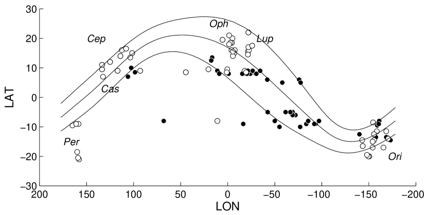
Figure 1: Galactic longitude and latitude distribution of the nearby HI (black dots) and H₂ (white dots) clouds. The dots mark the direction of peak emission. Clouds at $|b|<5\degr$ or $8\degr$ have not been selected. The curves follow the trace of the Belt across the sky as obtained from the best fit. The upper and lower lines mark the corresponding edges of the 60 pc thick disc of the Belt.

Varying the initial expansion parameters, the geometry and velocity field of the evolved Belt (today) have been compared with the space and velocity distributions of the nearby HI and H₂ clouds. Because the direction of these clouds is known, but rarely their distance, we developed a specific maximum-likelihood test to compare their direction and radial velocity with those of the modelled Belt sections. The likelihood expression is based on the probability $\Psi_{ij}$ for a cloud $i$ to be seen at relative distance $D_{ij}$ from an elementary Belt section $j$, and at a relative radial velocity $v_{ij}$ with respect to that of the Belt section (c.f. Equation 3). Gaussian probability density functions have been adopted in relative distance and relative radial velocity with standard deviations $\sigma_{D}=20$ pc and $\sigma_{v}=1$ km s^-1, respectively. So, $\Psi_{ij}$ is given by

$$\Psi_{ij} = \frac{g_{s}}{4\;\pi^{2}\;\sigma_{D}^{3}\;\sigma_{v}}\;e^{-\frac{D_{ij}^{2}}{2\;\sigma_{D}^{2}}}\;e^{-\frac{v_{ij}^{2}}{2\;\sigma_{v}^{2}}}$$ (3)

where $1/g_{s}$ is the Belt perimeter.

When the cloud distance to the Sun, $D_{i}\pm\Delta D_{i}$, is available (c.f. Tables 4 and 5), the cloud likelihood is obtained by integrating over the 60 Belt sections:

$$\mathcal{L}_{i} = \int_{Belt}\;\Psi_{ij}\;D_{i}^{2}\;\Delta\Omega_{i}\;\Delta D_{i}\;\Delta v_{i}\;ds_{j}$$ (4)

$\Delta\Omega_{i}=\Delta l_{i}\;\Delta b_{i}\;\cos b_{i}$ represents the 1 $\sigma$ confidence solid angle around the direction ($l_{i},b_{i}$) of peak emission in the cloud, in Galactic coordinates. $\Delta v_{i}$ notes the 1 $\sigma$ error on the observed cloud centroid velocity.

For a cloud with no distance estimate, we performed a Gauß-Legendre integration of the spatial probability density function along the cloud $(l_{i},b_{i})$ direction:

$$\mathcal{L}_{i} = \int_{Belt}\left[\frac{g_{s}}{4\;\pi^{2}\;\sigma_{D}^{3}\;\sigma_{v}}\;e^{-\frac{v_{ij}^{2}}{2\;\sigma_{v}^{2}}}\;\Delta\Omega_{i}\;\Delta v_{i}\;\;\;\;\cdots\right.$$

$$\cdots \left.\int_{\delta=0}^{+\infty}\delta^{2}\;e^{-\frac{(\delta\cos l_{i}\cos b_{i}-x_{j})^{2}}{2\;\sigma_{D}^{2}}}\;\;\;\;\cdots\right.$$ (5)

$$\cdots \left.e^{-\frac{(\delta\sin l_{i}\cos b_{i}-y_{j})^{2}}{2\;\sigma_{D}^{2}}}\;e^{-\frac{(\delta\sin b_{i}-z_{j})^{2}}{2\;\sigma_{D}^{2}}}\;d\delta\right]\;ds_{j}$$

$x_{j}$, $y_{j}$, and $z_{j}$ note the cartesian coordinates of the centre of a Belt section.

The likelihood $\mathcal{L}(\varphi_{0},l_{\Omega}^{0},H,d_{c}^{0},l_{c}^{0},\tau,M_{0},v_{0})$ of a model is obtained by the product of individual (independent) cloud probabilities $\mathcal{L}_{i}$. The maximum likelihood is found using the downhill simplex method developed by Nelder & Mead (1965). The iteration stops when the difference between the function values at each point of the simplex and the current minimum are less than $10^{-3}$. This procedure has been successfully tested using simulated clouds randomly generated from a known Belt.

3 Cloud selection

As noted by several authors, the Gould Belt has left its imprint on the local gas dynamics as seen in the HI data. The local molecular clouds, as mapped in CO, appear to follow a longitude-velocity pattern similar to that of the atomic gas in the Lindblad ring (Dame et al. 1987). To include all nearby atomic and molecular clouds, we used the extensive CO survey of the Milky Way at $|b|<25\degr$ by Dame et al. (1987) and two complementary HI surveys (Hartmann & Burton 1997; Strong et al. 1982) to cover the whole sky. Clouds were systematically searched for and isolated using the powerful clumpfind tool developed by Williams et al. (1994). This algorithm searches for coherent peaks of emission based on closed contours in a longitude-latitude-velocity data cube, from the highest intensity to the lowest. The algorithm yields the position of peak emission and centroid radial velocity of the clouds.

The CO data cube was processed in the $[-15,+17]$ km s^-1 velocity range characteristic of the local medium. The temperature increment for the clumpfind to follow down the intensity levels was set to $\Delta T=1$ K. The same procedure was applied to the HI data cubes for velocities $|v|<20$ km s^-1 and latitudes restricted to $|b|>3\degr$ to leave out extensions to medium latitudes of background clouds in the Galactic plane. Temperature steps of $\Delta T=0.07$ K and $\Delta T=2$ K have been used for the Hartmann & Burton (1997) and the Strong et al. (1982) surveys, respectively.

Table 1 summarizes the selection criteria used in longitude, latitude and velocity to avoid contamination from background clouds in the Galactic disc or in the Local Arm. These cuts were kept minimal to limit biases and to avoid an a priori selection of clouds obviously linked to the Belt while retaining the intrinsic spatial and velocity dispersion of the clouds in our neighbourhood. The lists of selected HI and H₂ clouds and their characteristics are given in Tables 4 and 5, respectively. The (l,b) directions and velocities of the selected clouds are displayed in Figures 1 and 2.

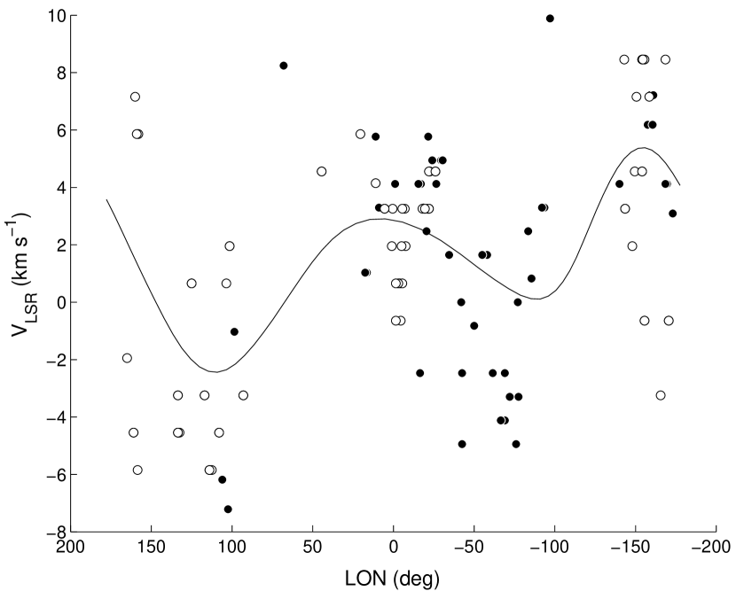
Figure 2: longitude-velocity distribution of the nearby HI (black dots) and H₂ (white dots) clouds and the best fit to the Belt rim kinematics. Projected velocities are given in the Local Standard of Rest.

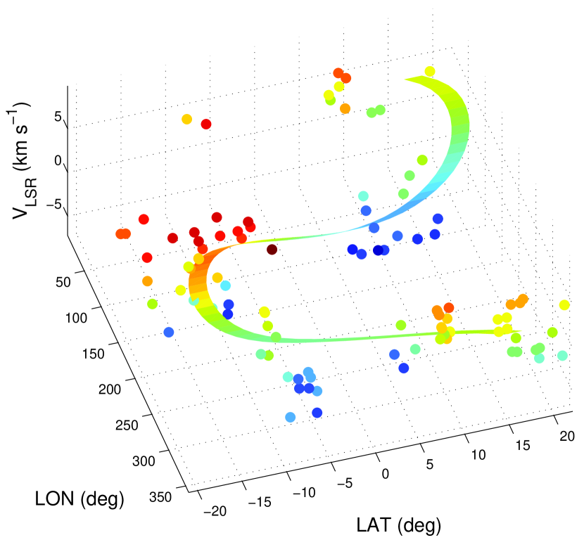
Figure 3: longitude, latitude, and velocity distribution of the nearby HI (black dots) and H₂ (white dots) clouds and the best fit to the Belt rim kinematics. Projected velocities are given in the Local Standard of Rest and are colour-coded from black to white from negative to positive values

4 Results and discussion

The initial and current characteristics of the Belt expansion that best fit the present-day cloud data are given in Table 2. The resulting geometry and dynamics appear to be independent of the presence or not in the fit of the Taurus clouds which, since they lie near the centre, do not participate to the expansion of the Belt rim . The quoted 1$\sigma$ errors are purely statistical and have been determined from the log-likelihood ratios and the information matrix (Strong 1985).

Figure 4 shows the maximum-likelihood evolution of the Belt rim, as seen at different epochs in a plane perpendicular to the Galactic one. The current Belt geometry is close to that depicted in the T = 30 Myr plot and the last plot illustrates how the Belt may fall back onto the Galactic disc within 10 to 15 Myr. The height that best fits the data is $H=60\pm 1$ pc. The expansion proceeds faster at higher $z$ altitudes because of the reduced ambient interstellar density. The inclined Belt starts by rapidly expanding out of the Galactic disc. Its shape gradually narrows into an ellipse that precesses because of the swept-up momentum from the interstellar gas and its differential rotation. The inclination also decreases with time and the disc gets clearly warped because of the gravitational pull from the Galactic disc.

To zeroth order, the expansion radius R(t) is well described by momentum conservation in a uniform medium of density $\rho$: $\frac{d}{dt}(\pi\rho HR^{2}\dot{R})=0$. The resulting power-law dependance $R\propto t^{1/3}$ is found in very good agreement with the evolution of the average size, R(t)=(a+b)/2, obtained from the model after the first 200 kyr.

The best fit yields a position and velocity field for the present Belt that are in good agreement with the cloud data, as illustrated in Figures 1, 2, and 3. Figure 1 shows the trace of the Belt across the sky in longitude and latitude. Apart from a few points, which have not been removed from the sample to avoid biases, the modelled Belt geometry nicely fits the data. Its angular width increases at low longitudes where the rim is closer and the varying angular width matches the angular dispersion seen in the nearby clouds. Figure 2 shows the cloud distribution in longitude and velocity, as well as the velocity field of the present rim. The slow expansion of the Belt to date reproduces the double-peaked velocity pattern over all longitudes. The velocity pattern clearly differs from the $v_{LSR}=A.d.sin(2l).cos^{2}(b)$ dependence expected from a pure differential rotation. The difference reflects the tilt of the Belt and its expansion. The peak-to-peak velocity amplitude is, however, not quite satisfactory, even in the face of the large intrinsic dispersion in the cloud data. This aspect will be addressed in section 4.2. Figure 3 shows that the model reasonably reproduces the complex data distribution in the longitude, latitude, and velocity phase space.

Table 2: Initial and present characteristics of the Gould Belt

	initially	today
$l_{\Omega}$ ($\degr$)	$290.1\pm 1.1$	$296.1\pm 2.0$
$\varphi$ ($\degr$)	$35.2\pm 0.3$	$17.2\pm 0.5$
$l_{c}$ ($\degr$)	$129.7\pm 2.0$	$180.4\pm 2.0$
$d_{c}$ (pc)	$145\pm 4$	$104\pm 4$
$a$ (pc)		$373\pm 5$
$b$ (pc)		$233\pm 5$
$\tau$ (Myr)	$E_{i}$ ($10^{45}$ J)	$H$ (pc)
$26.4\pm 0.4$	$1.0\pm 0.1$	$60\pm 1$

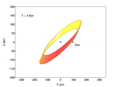
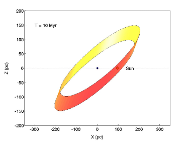
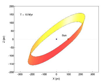
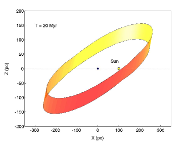
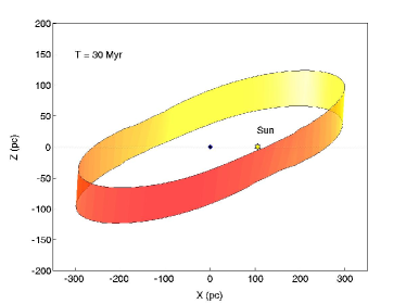
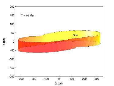
Figure 4: The Gould Belt evolution as seen at different epochs after the outburst, in a plane perpendicular to the Galactic plane, centred on the Belt centre. The x axis points to the Galactic centre and the location of the Sun is marked by an asterisk. The Belt expands and is further distorted by the combined effects of the Galactic differential rotation, interstellar density gradients above the Galactic plane, and the gravitational pull of the Galactic disc. The plot for 30 Myr is representative of the present-day geometry.

4.1 Geometry

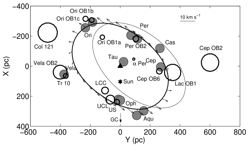
Figure 5: Present position of the Gould Belt projected on the Galactic plane. The x and y axes point to the Galactic Centre and in the direction of the Galactic rotation, respectively. Both are centred on the Belt centre. The velocity field outlines the Belt expansion with respect to the Local Standard of Rest. Nearby OB associations are plotted as thick circles using Hipparcos estimates of their distance and dimensions from de Zeeuw et al. (1999). The shaded circles mark the location of the main nearby H₂ cloud complexes. The thick and thin ellipses note the Belt rim as obtained in this work and earlier from the HI data by Olano (1982). The triangle and star note the Belt centre and the Sun, respectively.

The present ellipse has a semi-major axis $a=354\pm 5\;\mathrm{pc}$ and a semi-minor axis $b=232\pm 5\;\mathrm{pc}$, in good agreement with the dimensions of 360 by 210 pc and 341 by 267 pc derived by Olano (1982) and Moreno et al. (1999) from the sole HI data when modelling the expansion of a 2D ring in the Galactic plane or a 3D superbubble. The maximum-likelihood fit also yields a present inclination $\varphi=17.2\degr\pm 0.3\degr$ on the Galactic plane that nicely compares with the stellar estimates. Inclinations of 22.3$\degr$, $16\degr-22\degr$, and $20\degr$ have been found from the massive-star population by Comerón et al. (1994), Torra et al. (2000), and Olano (2001), respectively. A lower value of $12.5\degr$ was derived from the molecular clouds (Taylor et al. 1987). The difference with the present result can be attributed to a different cloud dataset. Taylor et al. did not select high-latitude dark clouds that are shown below to be consistent with the Belt shell. An inclination near $20\degr$ supports a strong connection between the Gould Belt and the Local Bubble (or Chimney) since the axis of the latter appears to be perpendicular to the Belt plane (Sfeir et al. 1999).

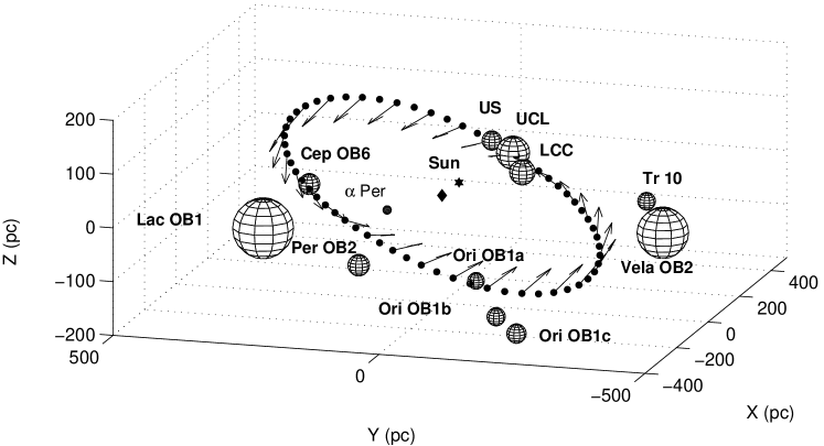
Figure 6: 3D view of the present Belt wave and its velocity field (with respect to the LSR) amid the local OB associations that are marked as spheres with a radius equal to their size (de Zeeuw et al. 1999). The diamond and star note the Belt centre and the Sun, respectively.

We find a position and orientation that significantly differ from previous estimates. The Belt centre is found at a distance $d_{centre}^{today}=104\pm 4$ pc from the Sun, in the direction $l_{centre}^{today}=180\degr\pm 2\degr$. More distant centres, well into the second quadrant, were proposed from the HI data by Olano (1982) and Moreno et al. (1999) (131 pc and 173 pc away, towards $166\degr$ and $117\degr$, resp.). The ellipse axes also point to a different direction. Figure 5 gives the current Belt position projected onto the Galactic plane. The change in orientation can be attributed to the refined distance information used here and to the presence of new major nearby H₂ complexes, such as Cepheus, Cassiopeia, and Polaris. Taylor et al. (1987) did not select their dark clouds as Belt members on a direction basis, but their combined direction, velocity, and distance appear here to be quite consistent with their being part of the expanding shell in the second quadrant (see Figures 1 and 2).

Finally, the best fit yields an ascending node longitude $l_{\Omega}=296.1\degr\pm 2.0\degr$ that is $\sim 10\degr$ higher than the values obtained from the stars ($l_{\Omega}=284.5\degr$ from the massive ones (Comerón et al. 1994) and $l_{\Omega}=282\degr$ from the young low-mass stars (Guillout et al. 1998)). The difference possibly reflects the time-lag between the stellar birth epoch and the slowly precessing rim today.

As shown in Figure 5, the position of the shell nicely coincides with most of the nearby OB associations such as Per OB2, Ori OB1a & OB1c, LCC, UCL, US, Cep OB6, Tr 10, Vela OB2, the positions of which are known from Hipparcos measurements (de Zeeuw et al. 1999). Col 121 and Cep OB2 clearly lie outside the Belt. Projections can be misleading. The 3D view displayed in Figure 6 illustrates that Lac OB1, often quoted in relation to the Belt, lies on the wrong side of the Galactic plane to be part of it, even when taking into account the Belt thickness of 60 pc. The old age of the association, of the order of 12–16 Myr (de Zeeuw et al. 1999), also confirms that Lac OB1 is not related to the Belt.

Table 3: Maximum likelihood values reached for different scenarii. P is the probability that random fluctuations from a given model fit the data as well as the expansion model. Characteristic Belt parameters are given for a selection of scenarii.

	$v_{rot}$ (km/s)	$\ln(L_{max})$	$P$	$\tau(Myr)$	$E_{i}$ ($10^{45}$ J)	$\varphi_{today}(\degr)$	$a_{today}$ (pc)	$b_{today}$ (pc)
expansion	0	-625.5		$26.4\pm 0.4$	$1.0\pm 0.1$	$17.2\pm 0.5$	$373\pm 5$	$233\pm 5$
rotation	5	-626.2	25.4%
rotation	50	-625.9	35.9%
rotation	-50	-625.6	77.7%	$26.4\pm 0.5$	$1.1\pm 0.1$	$17.3\pm 0.5$	$372\pm 6$	$232\pm 6$
rotation	100	-626.0	34.8%
rotation	-100	-625.5	100%	$26.4\pm 0.5$	$1.0\pm 0.1$	$17.1\pm 0.5$	$371\pm 5$	$232\pm 5$
plane crossing	0	-936.3	$\ll$	$51.8\pm 1.0$	$0.6\pm 0.06$	$15.1\pm 0.7$	$304\pm 6$	$219\pm 6$
fragmentation	0	-667.6	5e-20	$28.9\pm 0.6$	$0.3\pm 0.03$	$5.7\pm 0.5$	$142\pm 5$	$72\pm 5$

4.2 Effects of an initial rotation, shell fragmentation and Galactic plane crossing

The velocity dispersion of the data points in Figure 2 is large, but consistent with the cloud to cloud dispersion observed in the interstellar medium. A larger peak-to-peak amplitude in the shell velocity would, however, better represent the data. The influence of the initial conditions, the Belt thickness, the distance information, and the interstellar density profiles have been investigated to reduce this discrepancy, but none of these options leads to a significant increase in velocity amplitude within sensible limits. The only sensitive parameter is the Oort’s constant A, but unrealistic values beyond 17 km s^-1 kpc^-1 are required to slightly improve the fit. Other scenarii have been studied.

One possibility was to allow the Belt to cross the Galactic plane before reaching its present orientation. The effect of an initial rotation has also been considered by adding a tangential component to the initial expansion velocity. A more realistic braking of the shell has been introduced in the late stages of the evolution by gradually applying a drag force on the shell elements when their velocity falls into the 30 to 10 km s^-1 interval. In parallel, shell fragmentation has been implemented by increasing the porosity to the interstellar flow. The porosity coefficient $\alpha_{p}$ varies linearly from a pure snowplough case above 20 km s^-1 ($\alpha_{p}=0$) to a pure drag without accretion below 5 km s^-1 ($\alpha_{p}=1$). The drag force is given by $\overrightarrow{dF}=-\alpha_{p}\;C_{x}\;\rho_{gas}\;(\overrightarrow{v}^{\prime}\cdot\overrightarrow{dS})\;\overrightarrow{v}^{\prime}$ where $C_{x}$ denotes the friction coefficient. A value of 0.5 was adopted corresponding to turbulent friction on a sphere. $\overrightarrow{dS}$ is an elementary surface of the shell front, pointing outwards, and $\overrightarrow{v}^{\prime}$ gives the relative velocity of $\overrightarrow{dS}$ with respect to the interstellar medium.

The maximum-likelihood values reached for these different scenarii are given in Table 3. Probabilities for random fluctuations from a model to fit the data as well as the original expansion model are estimated from the likelihood ratio $-2\;\ln\lambda=-2\;\ln(\mathcal{L}_{max\,model}/\mathcal{L}_{max\,exp})$ between the two models. This ratio follows a $\chi^{2}_{1}$ distribution (Eadie et al. 1971). The corresponding probabilities are given in Table 3. It can be seen that a scenario including a late shell fragmentation or a Galactic plane crossing can hardly reproduce the data. The improvement in the quality of the fit of the expansion model over these scenarii is very significant.

Because of the reduced deceleration of the fragmented shell, a lower initial velocity is needed to match the low cloud velocities and the small size and low inclination resulting for the evolved Belt in this case explain the much poorer fit.

The crossing of the Galactic plane results in an hour-glass like distorsion of the shell because of the interstellar density gradient implying different expansion velocities in and out of the Galactic disc. A maximum-likelihood solution could, however, be found. It requires a larger initial inclination to boost the Belt to larger altitudes and make use of the increased gravitational pull towards the plane to cross it and reach a 20$\degr$ tilt on the other side. A lower initial kinetic energy is needed because of the extra energy provided by the disc torque. The evolved Belt disc ends up being quite warped. As expected from Figure 7, the resulting fit is much poorer than without plane crossing. This is confirmed by a dramatic decrease in the maximum likelihood. This scenario requires a substantially longer time span of $51.8\pm 1.0$ Myr.

The fit seems rather insensitive to an initial rotation, even for large rotation velocities comparable to the expansion one. The age and energy estimates, as well as the final geometry, are not affected by an initial rotation. This set of results show that the dominant factor in the shell dynamics and final velocity distribution is the momentum accreted from the interstellar gas.

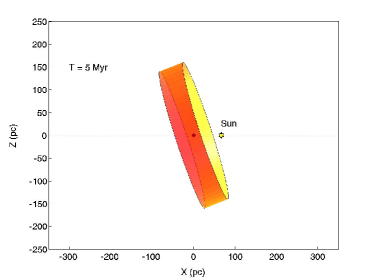
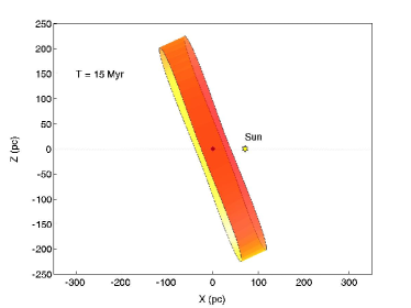
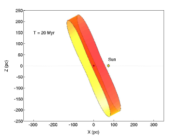
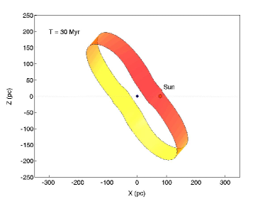
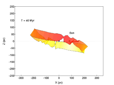
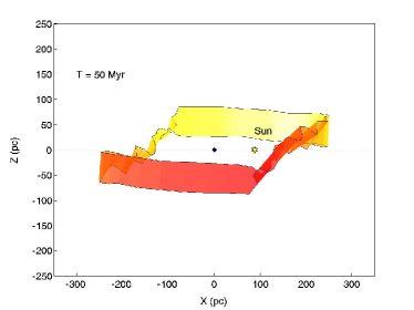
Figure 7: The Gould Belt evolution as seen at different epochs after the outburst (see Figure 7), assuming a crossing of the Galactic plane. The plot for 50 Myr is representative of the present-day geometry.

4.3 Age of the Belt

The best value found for the age of the Belt, $\tau=26.4\pm 0.4$ Myr, is comparable to previous estimates based on the gas dynamics (31-36 Myr in the 2D model of Olano (1982), 23 Myr and 15.5 Myr in the 3D superbubble model of Moreno et al. (1999), without and with interstellar pressure). The shorter timescales involved in the 3D models may be due to the faster expansion in the rarefied medium away from the Galactic disc in the early stages. So, the age estimate is sensitive to the interstellar stratification. The dynamics of the stellar system, mainly its vertical oscillations and estimates of the Oort constants, imply an age of $34\pm 3$ Myr (Comerón 1999). Taken together, these various measurements suggest a dynamical age of the Belt of order 30 Myr.

Yet, stellar ages point to a twice longer timescale for the Belt system. Determining the age of the massive stars from photometric measurements, Westin (1985) proposed an upper limit of 60 Myr, and Torra et al. (2000) showed that 60 to 66% of the stars younger than 60 Myr and closer than 600 pc belong to the Belt. The X-ray luminosities of $10^{30.5\pm 0.5}$ erg/s of the young low-mass stars correspond to ages between 30 and 80 Myr (Guillout et al. 1998). One difficulty in determining the Belt age from the stars is to reliably separate the Belt and the Galactic populations. Another comes from deriving the photometric age without properly taking into account the stellar rotation. Figueras & Blasi (1998) indeed found that photometric ages of rotating B7-A4 stars are overestimated by 30 to 50% on average. This important bias would also affect the highly rotating massive stars and would help reduce the discrepancy between the dynamical age of $\sim 30$ Myr and the stellar age of $\sim 60$ Myr. On the other hand, an origin in a single explosive event or continuous energy injection would imply different dynamical ages. As discussed in the next section, gradual injection would further reduce the dynamical timescale. One way to reduce the dynamical and stellar age discrepancy is to allow the Belt to cross the Galactic plane before reaching its present orientation. The much poorer fit for this scenario, however, does not support this possibility.

4.4 Input energy

The expansion results from an initial kinetic energy input of $(1.0\pm 0.1)$ $10^{45}$ J which is comparable, but slightly higher than the energy of 6.1 10⁴⁴ J required in the 2D expansion model of Olano (1982). This is due to the extra amount of work needed to expand against the gravitational pull of the Galactic disc in the early phases. An equivalent energy of 6 10⁴⁴ J is required for the 3D expansion of a superbubble, in a 3 times lower interstellar density, but against ambient pressure (Moreno et al. 1999). The 10 times lower value they found for pressureless expansion is due to their choice of a very low density. An initial energy of $10^{45}$ J is typical of the energy deposit from multiple supernovae inside a young stellar cluster, but it would require a series of explosions within a rather short period. The energy budget is also typical of a hypernova powering a $\gamma$-ray burst event. Exploring whether the asymetrical explosion can explain the Belt tilt is under study. The energy budget can also be accounted for by the potential energy of high-velocity clouds falling on the Galactic disc (Comerón & Torra 1992; Comerón et al. 1994).

Continuous energy injection by multiple supernovae and expansion into a highly inhomogeneous medium would yield a larger dynamical range in velocity. Injecting energy gradually would, however, accelerate the Belt expansion. To zeroth order approximation, expansion in a uniform medium of density $\rho$, with constant power injection $P_{inj}$, can be modelled by $\frac{d}{dt}(\pi\rho HR^{2}\dot{R})=2\pi HRp_{int}$, where $p_{int}$ represents an internal source of pressure to account for the energy deposit. Its mechanical power is $2\pi HRp_{int}\dot{R}=P_{inj}$. Solving for power-law expansion ($p_{int}\propto{R^{-\gamma}}$ and $R\propto{t^{n}}$), one finds a faster expansion $R\propto{t^{3/4}}$ for constant power injection than from a single explosion ($R\propto{t^{1/3}}$). The faster evolution would further reduce the dynamical age with respect to the stellar age, and also reduce the Belt eccentricity with respect to the location of the clouds and OB associations. The complex interplay between the power injection and momentum accretion is being investigated.

4.5 Mass accretion

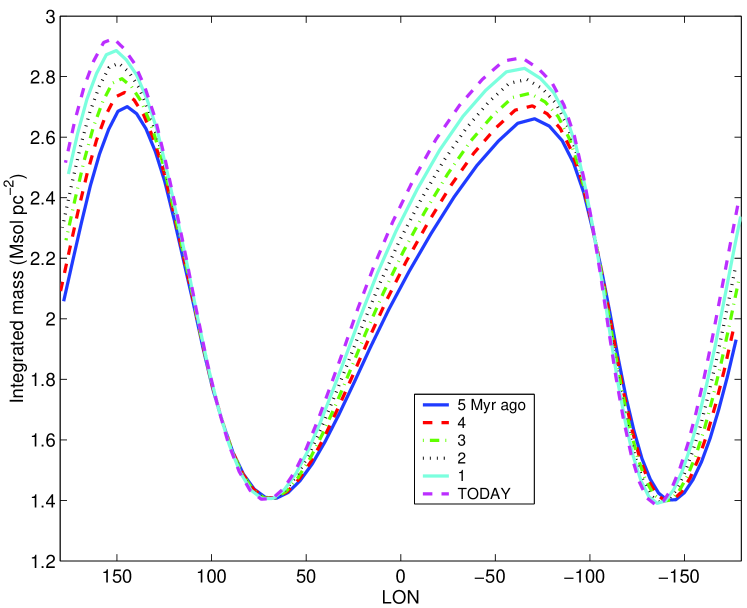
Figure 8: Total integrated mass along the Gould Belt rim, in solar masses per pc², in the snowplough case, at five different epochs over the past 5 Myr.

The swept-up mass in the evolved shell is found to be 2.4 10⁵ M_⊙. The larger value of 1.2 10⁶ M_⊙ proposed by Olano (1982) results from his choice of a 20 % larger density in the Galactic plane and the absence of vertical gradients and expansion away from the plane. The estimate of 3.3 10⁵ M_⊙ found by Moreno et al. (1999) in the 3D supershell is close to our result. The 3 times lower density value they adopted is compensated by the lack of vertical gradients.

Figure 8 shows the integrated mass distribution along the Belt over the past 5 Myr. The mass accumulated in the snowplough case is lowest in the directions $35\degr<l<100\degr$ and $-155\degr<l<-110\degr$. These regions in the first and third quadrants are indeed relatively free of major cloud complexes (c.f. Figure 5). Conversely, the swept-up mass is highest in the $-100\degr<l<22\degr$ and $-165\degr<l<115\degr$ intervals that encompass most of the main nearby complexes. The nodal line of maximum accretion is close to the Belt nodal line, illustrating the importance of the Belt tilt and of the vertical density gradient. In other words, the Belt accretes more near the Galactic disc. Figure 8 illustrates the Belt precession, of the order of a few degrees per Myr, that can be attributed to the Galactic differential rotation.

4.6 The Belt wave and the OB associations

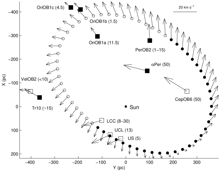
Figure 9: Present-day velocities (projected on the Galactic plane) of the nearby OB associations (squares) (de Zeeuw et al. 1999), and of stars that would have been born in the expanding Belt shell 10 Myr ago. Their position (circles) and velocity today have been computed after ballistic motion in the Galactic potential. All velocities are corrected for solar motion and Galactic rotation. Filled and open symbols mark negative and positive vertical $v_{z}$ velocities, respectively. The presumed age for each OB association is given in Myr. The Sun is marked by a star.

The velocity field of the nearby young stellar groups (see Figure 5 in Lindblad et al. (1997)) suggests a stream-like motion spreading out of the Belt region. Because of the frictionless motion of the stars in the Galactic potential, one expects older stellar groups, born in a faster expanding Belt shell, to travel farther out than younger groups born from a slowed-down Belt. The opposite situation is observed in Figure 9 where younger OB associations are found at larger radii than older ones (notice in particular the LCC/UCL/US and the Ori1 a/b/c sequences). The present-day positions and velocities of stars born 10 Myr ago from the expanding shell have been computed from their ballistic motion in the Galactic potential. Note that velocities were corrected for solar motion (using $U_{x\odot}=10$ km $s^{-1}$, $V_{y\odot}=5$ km $s^{-1}$, and $W_{z\odot}=-7$ km $s^{-1}$) and for Galactic rotation (using Oort’s constants $A=14.8$ km s^-1 kpc^-1 and $B=-12.4$ km s^-1 kpc^-1) in order to allow a direct comparison with Figure 29 from de Zeeuw et al. (1999). It implies that velocities are considered with respect to the Local Standard of Rest at the position of the object considered. One expects the computed present-day positions to be systematically too far out because the Belt shell model has been fitted against the current position of the OB associations, not against their birth positions several Myr ago. There is, however, no convincing correlation between the observed and expected velocity fields, particularly in the vertical velocity component due to the gravitational pull from the Galactic disc. The current data suggests that the Belt wave triggers star formation when overtaking a cloud and that the association average velocity does not relate to that of the progenitor cloud.

5 Conclusion

The Gould Belt expansion has been modelled in 3D and has been fitted against the current direction and velocity of the H₂ and HI clouds that are found in the solar neighbourhood. Distance measurements have also been used for a subset of clouds. Due to the combined effects of the Galactic differential rotation, its gravitational pull, and the interstellar density gradients, the present Belt section has evolved into a slightly warped ellipse, with semi-axes of $(373\pm 5)$ pc and $(233\pm 5)$ pc, and an inclination of $17.2\degr\pm 0.5\degr$. Its centre is currently located $(104\pm 4)$ pc away from the Sun, in the direction $l_{centre}=180.4\degr\pm 2.0\degr$. The thickness that best fits the data is $H=(60\pm 1)$ pc. While these characteristics nicely compare with previous estimates, a different Belt orientation has been found that is driven by the presence of new major H₂ complexes and the revised distance information used here from Hipparchos measurements. The Belt position and orientation are found to coincide with the main OB associations and molecular clouds in our vicinity. A larger velocity amplitude would better represent the gas pattern, but it turns out to be insensitive to all model ingredients but for the Oort constant A. Other scenarii have been tested including shell fragmentation in the late stages, an initial rotation, or the crossing of the Galactic disc. They did not yield an increase in the final dynamical range in velocity. Much poorer fits to the data were obtained for the fragmented shell and the disc crossing cases. The Belt evolution has been compared to the kinematics of the nearby OB associations. Its expansion appears to have no influence on the observed average stellar motions. On the other hand, the swept-up mass distribution along the Belt rim, for a total of 2.4 $10^{5}$ M_⊙, is reasonably consistent with the cloud distribution. The younger OB associations are surprisingly found farther away from the Belt centre than the older ones.

The initial kinetic energy of $E_{i}=(1.0\pm 0.1)$ 10⁴⁵ J amounts to that of 10 supernovae, as previously proposed by several authors. The dynamical age of $(26\pm 0.4)$ Myr is equivalent to earlier estimates based on the gas expansion, but it is only half of the 60 Myr age derived from photometric stellar ages. This discrepancy does not result from the choice of a single explosion at the origin. Continuous energy injection would increase the discrepancy by further reducing the dynamical age. The age estimate is not sensitive to an initial rotation either. Allowing one crossing of the Galactic disc before reaching the present inclination implies a dynamical age of 52 Myr in better agreement with the stellar ages, but the very poor fit does not support this possibility. Important biases in the photometric derivation of stellar ages for rapidly rotating stars have been reported that could help solve this discrepancy.

Appendix A CLUMPFIND results

For each clump detected with clumpfind, the position and velocity of the corresponding centroid are given in the following Tables. For known molecular complexes, distances that were used in the likelihood function (c.f. section 2.4) are also indicated.

Table 4: HI clumps

l	b	vLSR	D	complex
(deg)	(deg)	(km/s)	(pc)
98,5	8,5	-1,030529	?
106	7	-6,18318	?
16,5	13,5	1,030531	?
17,5	12,5	1,030531	?
102,5	10	-7,21371	?
-169,5	-13,5	4,122121	340	Ori
-159	-9,5	7,213711	500	Oria
-173	-14,5	3,091591	340	Ori
-157,5	-13,5	6,183181	500	Oria
-140	-12,5	4,122121	?
-168,5	-13,5	4,122121	340	Ori
-161	-8	7,213711	?
-160,5	-9	6,183181	?
68	-8	8,244241	?
-76	6	-4,943996	?
-77,5	5	-3,295996	?
-17	8	4,120004	?
-18,5	9	3,296004	140	Lupb
-24	8	4,944004	140	Lupb
-1	8	4,120004	125	Ophc
-21,5	9	5,768004	140	Lupb
-15,5	8	4,120004	?
-20,5	8	2,472004	?
-29,5	8	4,944004	?
-26,5	9	4,120004	?
-30,5	8	4,944004	?
11	9	5,768004	?
-58	5	1,648004	?
-34,5	9	1,648004	?
9	8	3,296004	?
-42	6	0,000004	?
-93,5	-9	3,296004	380	Vela
-97	-8	9,888004	380	Vela
-92	-9	3,296004	380	Vela
-42,5	-5	-4,943996	?
-83,5	-9	2,472004	?
-72	-6	-3,295996	?
-42,5	-5	-2,471996	?
-69	-5	-2,471996	?
-85,5	-8	0,824004	?
-69	-6	-4,119996	?
-77	-10	0,000004	?
-66,5	-5	-4,119996	?
-61,5	-5	-2,471996	?
-50	-8	-0,823996	?
-16,5	-9	-2,471996	?
-55	-10	1,648004	?

• Maddalena et al. (1986)

• Murphy et al. (1986)

• de Geus et al. (1990)

Table 5: CO clumps

l	b	vLSR	D	complex
(deg)	(deg)	(km/s)	(pc)
11	-8	4,1466	?
133,5	9,5	-4,5462	350	Casa
114	14	-5,8466	300	Cepa
-26	17,5	4,5566	?
-170,5	-14	-0,645	340	Ori
101,5	15	1,9558	300	Cepa
-154	-15	4,5566	500	Orib
108	16,5	-4,5462	300	Cepa
161	-9	-4,5462	320	Perc
-22	22	3,2562	?
-19,5	8,5	3,2562	140	Lupd
125	12	0,6554	350	Casa
5,5	19,5	3,2562	?
93	9	-3,2458	?
117	9	-3,2458	?
133,5	11	-3,2458	350	Casa
44,5	8,5	4,5566	?
-155,5	-12,5	-0,645	?
-143,5	-16,5	3,2562	?
-154	-17	8,4578	500	Orib
-150,5	-20	7,1574	500	Orib
-7,5	16	1,9558	125	Ophe
-7	15	3,2562	125	Ophe
-149,5	-20	4,5566	?
-155,5	-14,5	8,4578	500	Orib
-21,5	15,5	3,2562	?
158	-21	5,857	320	Perc
-148	-19,5	1,9558	?
-18	9	3,2562	140	Lupd
-5	20	1,9558	125	Ophe
-4	16	0,6554	125	Ophe
-22,5	16	4,5566	?
-5,5	14	3,2562	125	Ophe
-168,5	-11,5	8,4578	?
-21,5	14,5	3,2562	?
159	-20,5	5,857	320	Perc
-4,5	18,5	-0,645	?
160	-18,5	7,1574	?
-5,5	15,5	0,6554	125	Ophe
-3	18,5	0,6554	125	Ophe
-22	17	4,5566	?
-165,5	-17	-3,2458	340	Ori
-1,5	21	-0,645	?
0,5	9,5	3,2562	125	Ophe
112,5	16	-5,8466	300	Cepa
-1,5	18	0,6554	125	Ophe
1	8,5	1,9558	?
165	-9,5	-1,9454	140	Tauf
103,5	13,5	0,6554	300	Cepa
-154,5	-8,5	8,4578	500	Orib
-143	-14,5	8,4578	?
20,5	9,5	5,857	250	Aqu

• Grenier et al. (1989)

• Maddalena et al. (1986)

• Ungerechts & Thaddeus (1987)

• Murphy et al. (1986)

• de Geus et al. (1990)

• Murphy & Myers (1985)

Table 6: CO clumps (continued)

l	b	vLSR	D	complex
(deg)	(deg)	(km/s)	(pc)
132,5	7	-4,5462	350	Casa
-158,5	-11,5	7,1574	500	Oric
158,5	-9	-5,8466	320	Perd
133,5	9,5	-4,5462	350	Cas
114	14	-5,8466	300	Cepb
-26	17,5	4,5566	?
-170,5	-14	-0,645	340	Ori
101,5	15	1,9558	300	Cepb
-154	-15	4,5566	500	Oric
108	16,5	-4,5462	300	Cepb
161	-9	-4,5462	320	Perd
-22	22	3,2562	?
-19,5	8,5	3,2562	140	Lupe
125	12	0,6554	350	Cas
5,5	19,5	3,2562	?
93	9	-3,2458	?
117	9	-3,2458	?
133,5	11	-3,2458	350	Cas
44,5	8,5	4,5566	?
-155,5	-12,5	-0,645	?
-143,5	-16,5	3,2562	?