ACBAR: The Arcminute Cosmology Bolometer Array Receiver

Abstract

We describe the Arcminute Cosmology Bolometer Array Receiver (Acbar); a multifrequency millimeter-wave receiver designed for observations of the Cosmic Microwave Background (CMB) and the Sunyaev-Zel’dovich effect in clusters of galaxies. The Acbar focal plane consists of a 16-pixel, background-limited, 240 mK bolometer array that can be configured to observe simultaneously at 150, 220, 280, and 350 GHz. With $4-5^{\prime}$ FWHM beams and a $3^{\circ}$ azimuth chop, Acbar is sensitive to a wide range of angular scales. Acbar was installed on the 2 m Viper telescope at the South Pole in January 2001. We describe the design of the instrument and its performance during the 2001 and 2002 observing seasons.

1 Introduction

The Arcminute Cosmology Bolometer Array Receiver (Acbar) was designed to make sensitive, high-resolution measurements of the microwave sky at multiple millimeter wavelengths. Observations of the cosmic microwave background (CMB) can provide a wealth of information about the Universe. Measurement of the angular power spectrum of the CMB allows us to determine the values of the cosmological parameters (such as the age, density, and composition of the Universe) within the context of models of the early universe.

The angular power spectrum of the CMB is exponentially damped on small angular scales by photon diffusion (Silk 1968; White 2001). On very small scales ($\lesssim 5^{\prime}$) it is believed the CMB power spectrum will be dominated by sources of secondary anisotropy. One such source is the scattering of CMB photons by the hot plasma in foreground clusters of galaxies [see, for example, Holder & Carlstrom (1999) or Cooray & Melchiorri (2002)] known as the Sunyaev-Zel’dovich (SZ) effect (Sunyaev & Zeldovich 1972; Birkinshaw 1999). Observations with the CBI and BIMA may have already detected this SZ power spectrum (Bond et al. 2002; Dawson et al. 2002; Komatsu & Seljak 2002; Mason et al. 2003). Multifrequency observations should allow the separation of the primary and SZ power spectra through the unique frequency dependence of the SZ effect.

The field of millimeter-wave bolometer observations of the CMB has a long pedigree with both ground-based [IRTF (Meyer et al. 1983), QMC-Oregon (Ade et al. 1984), IRAM (Kreysa et al. 1987), SEST/OASI (Pizzo et al. 1995), SuZIE (Holzapfel et al. 1997; Mauskopf et al. 2000), Python (Platt et al. 1997), SCUBA (Holland et al. 1999), and Diabolo (Benoit et al. 2000)] and balloon-borne experiments [TopHat (Cheng 1994), PRONAOS (Lamarre 1994), MSAM (Fixsen et al. 1996), MAXIMA (Lee et al. 1999), and BOOMERANG (Crill et al. 2002)]. The Acbar experiment drew upon much of this well-developed technology, thus enabling rapid construction and deployment of a very sensitive instrument.

The Acbar focal plane is a background limited, 16-pixel, 240 mK bolometer array that is configurable to observe simultaneously at 150, 220, 280, and 350 GHz with $4-5^{\prime}$ resolution. Observations at these frequencies span the peak intensities of CMB anisotropies and the SZ effects while avoiding foreground contaminants, such as dust and radio point sources (Tegmark & Efstathiou 1996). The technology, frequency coverage, and angular resolution of Acbar are very similar to those being used in the Planck HFI. Acbar was installed on the 2 m Viper telescope at the South Pole in January 2001. Acbar exploits the excellent polar atmospheric conditions and large $3^{\circ}$ telescope chop to measure angular scales from $\ell\sim 75$ to $\sim 3000$.

This paper describes the details of the instrumental design and performance of Acbar. The telescope and instrument were upgraded in December 2001 and we describe the performance during both the 2001 and 2002 observing seasons. We present the CMB power spectrum measured by Acbar in Kuo et al. (2002) and constraints on cosmological parameters derived from this data in Goldstein et al. (2002). We describe pointed observations of nearby clusters in Gomez et al. (2002) as well as a survey for clusters of galaxies with the SZ effect in Runyan et al. (2003).

We describe the physical environment at the South Pole in §2 and discuss the details of the telescope and focal plane optics in §3. The cryogenics employed to cool the detectors to 240 mK are described in §4 and the low-noise electronics are discussed in §5. In §6 and §7, we describe the observations during 2001 and 2002 as well as the calibration of the instrument. We present the achieved sensitivity of the instrument in §8 and our conclusions in §9.

2 The South Pole Environment

Acbar observes from the Viper telescope located at the Southern geographic pole in Antarctica. The South Pole provides a unique platform for terrestrial far-infrared observations. The Amundsen-Scott Station is located atop the Ross ice shelf at an elevation of $9,300^{\prime}$ which reduces the column depth of atmosphere above the telescope. The pressure elevation at the Pole can exceed $11,000^{\prime}$ due to the thinning of the polar atmosphere from the extreme cold and the bulging of the atmosphere at the equator. The cold temperature freezes out most of the precipitable water vapor from the atmosphere, greatly reducing emission and absorption at millimeter wavelengths. The ambient temperature averages near $-80^{\circ}$F in the austral winter with a precipitable water vapor less than 0.32 mm $\sim 75\%$ of the time (Lane 1998). In addition, the atmosphere is stable for long periods of time (Peterson et al. 2002) punctuated by short periods of poor weather (usually associated with a warming of the ambient temperature) and has no diurnal variation. The entire Southern celestial hemisphere is available year round allowing long, continuous observations of a field. Combined with a well established research infrastructure, these attributes make the South Pole arguably one of the best locations on the planet for millimeter-wave observations.

3 Optics

3.1 Telescope Optics

The Viper telescope is located less than one kilometer from the South Geographic Pole, in close proximity to the Amundsen-Scott South Pole station. Viper is an off-axis aplanatic Gregorian telescope with a re-imaging tertiary mirror to reduce the effective focal length. Viper has a 2 m diameter primary mirror and additional 0.5 m radius reflective skirt to reflect primary spillover to the sky. There is a chopping flat mirror located at the image of the primary formed by the secondary mirror which sweeps the beams approximately $3^{\circ}$ on the sky with little modulation of the beams on the primary (of order a few cm).

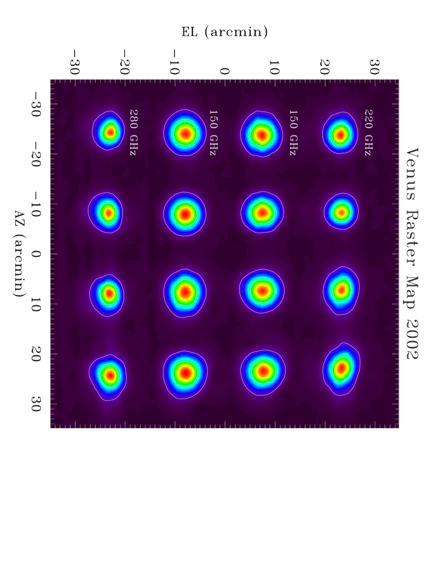
Figure 2: Raster map of Venus at an elevation of $19.8^{\circ}$ taken on 2002 September 22. The angular diameter of Venus was $37^{\prime\prime}$ on this date and the map has been smoothed with a $1^{\prime}$ FWHM Gaussian. The white contours correspond to power levels of 10% and 50%.

The re-imaging tertiary on the Viper telescope was originally designed for low frequency (40 GHz) observations of the CMB with a 2-pixel array (Peterson et al. 2000). The tertiary was redesigned using geometrical ray-tracing software to provide sufficient optical quality across a large field of view ($\sim 1~{}{\rm deg}^{2}$) at Acbar’s higher frequencies. With the new tertiary, the telescope has an effective focal length of 3.44 m, resulting in a plate scale of $\sim 1^{\prime}/{\rm mm}$. The 16 mm separation of feeds on the Acbar focal plane (see Figure 1) produces a $4\times 4$ array of beams separated by $\sim 16^{\prime}$ on the sky (see Figure 2).

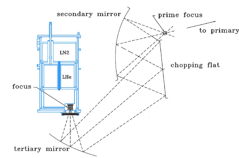
Figure 3: Most of the Viper telescope optics along with the Acbar cryostat. The light rays are the geometrical optic rays for full illumination of the 2 m primary and are shown to illustrate the tight clearance around the prime focus.

Figure 3 shows a schematic of a subsection the Viper telescope optics along with the Acbar receiver. The extreme geometric optical rays are drawn to illustrate the tight clearances of the system; the actual Gaussian beam widths are much more narrow than the lines drawn. With full illumination of the 2 m primary, the focal plane is fed at $f/1.7$ in the geometric optics limit. The primary illumination varies with frequency, however, and so the effective half-power $f/\#$ of the beams vary from $f/4.6$ at 150 GHz to $f/11.1$ at 350 GHz. The dewar is mounted on a sliding pillow-block mount with a linear focus actuator that controls the distance between the dewar and tertiary mirror.

The chopping flat mirror sweeps the beams across the sky approximately $1^{\circ}$ for every $2.2^{\circ}$ of chopper rotation. The position of the chopper is read out with an angular encoder and is controlled to trace a triangular chop with a PID loop. The triangle wave results in a constant-velocity chop across the sky. The chopper encoder waveform is fed into the data acquisition system as an additional signal and sampled at the same rate as the bolometers ($\sim 2400$ Hz). When observing the CMB we sweep the beams approximately $3^{\circ}$ across the sky in about a second, which effectively freezes the atmosphere. The chopper speed is chosen so that the beams will take multiple detector time constants to cross a point source. We employed a chopper speed of 0.7 Hz in 2001 and 0.3 Hz in 2002. When observing known clusters we shorten the chop length to $1.5^{\circ}$ to concentrate the observing time on the cluster as well as increase the chopper frequency to keep the scan velocity the same as for CMB observations.

During the 2001 season, we used an RVDT angular encoder as both the control signal and recorded position signal. The RVDT suffered from two features that were the dominant sources of pointing error in 2001. First, a drift in the zero-point voltage of the encoder caused the position on the sky corresponding to a fixed encoder voltage to change with time. This drift was slow (about 10^′ per month) and we were able to fit and correct for it with frequent observations of galactic sources. The second more serious problem was the fluctuation of encoder gain of about 8%. The gain of the encoder was roughly bimodal, falling into a high-gain or low-gain state. To determine the gain state of the encoder we compare the separation of a bright object (in volts) between two adjacent channels. To remedy these problems, we installed an absolute optical encoder for 2002. The RMS pointing error during 2001 was approximately 1.3^′ and the RMS for 2002 was 30^′′.

The telescope is enclosed in a large, conical ground shield that reflects telescope spillover to the sky. The ground shield also blocks emission from elevations below $\sim 25^{\circ}$. This reduces optical loading and the effects of modulated sidelobes. One section of the ground shield lowers to allow observations of low-elevation sources; this is necessary to observe planets which do not rise higher than $\sim 30^{\circ}$ above the horizon at the pole. Fortunately, most of the region of the Southern Hemisphere with the lowest dust contrast is located at $EL>25^{\circ}$ at the pole.

A servo-controlled PID loop controls the positioning of the telescope azimuth and elevation with power supplied by linear servo amplifiers. All temperature-sensitive components of the telescope are heated to $\sim 300$ K. The mirrors are equipped with heaters for sublimating the thin layer of ice that accumulates over time. Blowing snow collects on most of the mirrors and must be cleaned off daily; this prevents snow from contributing to chopper synchronous offsets as well as attenuating astrophysical signals, as discussed below in §6.2.

We developed a telescope pointing model using frequent observations of both galactic and extragalactic sources. This allows us to reconstruct the position of each beam on the sky using the reported telescope AZ, EL, and chopper encoder positions. The pointing model incorporates the distance of the telescope from the geographic pole, the tilt of the azimuth ring, flexure of the telescope with elevation, and the collimation offsets between the radio beams and nominal telescope boresight position. The measured AZ and EL chopper functions are then used to translate the measured chopper position into an instantaneous beam position for all 16 optical channels. Because of the proximity to the geographic pole, the telescope requires very little change in elevation while tracking a source across the sky.

3.2 Focal Plane Optics

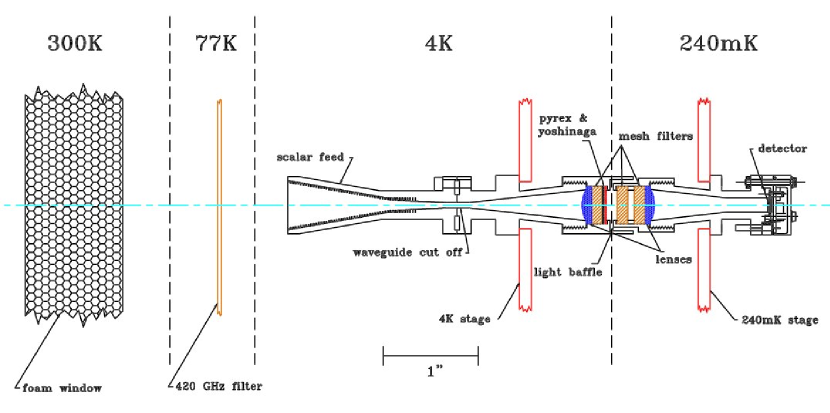
Figure 4: Acbar 150 GHz feed horn structure and warm filter arrangement for 2002. Dashed vertical lines indicate thermal boundaries.

The focal plane optics are designed to couple the Acbar receiver to the Viper telescope and produce diffraction-limited beams at 150 GHz. The angular resolution at higher frequencies is intentionally degraded to produce nearly matched beam sizes at all frequencies. Figure 1 shows the layout of the Acbar focal plane as configured for observations in 2001 and 2002. In 2001, the focal plane was arranged with common frequencies aligned in columns so that each row observed at 150, 220, 280, and 350 GHz as the chopper swept across the sky. For 2002, the 350 GHz feeds were replaced with an additional set of 150 GHz feeds (because of their poor noise performance). The focal plane was arranged with rows of common frequency to concentrate the declination extent of the 150 GHz channels in 2002. The design of the Acbar feed structure is based upon the Planck satellite prototype design of Church et al. (1996) (see Figure 4). The main optical elements of the focal plane are the beam defining scalar feeds, expanding and reconcentrating conical feeds, filters, and bolometric detectors. Each of these will be described in the following sections.

3.3 Scalar Feeds

Acbar’s corrugated feeds are designed to produce single-moded, nearly Gaussian beams with very low sidelobes. This reduces optical loading from telescope spillover and decreases offset signals from modulation of the spillover by the chopping flat of Viper. Gaussian illumination also results in the smallest beam sizes from an aperture. Figure 4 shows the Acbar 150 GHz scalar feed structure. The feeds were fabricated by Thomas Keating, Ltd. and performed well within specifications (see Table 1). The geometry of the conical section of the scalar feeds (aperture diameter and aspect ratio) is designed to produce primary mirror beam waists that scale with wavelength. We modeled the expected beam patterns by assuming balanced hybrid conditions at the aperture and used a Gauss-Laguerre expansion of the $HE_{11}$ mode as described in Wylde (1984). The aperture and length dimensions of all four feeds are also listed in Table 1. The corrugation geometry within the conical section is designed in accordance with Clarricoats & Olver (1984); the corrugation depth is $\lambda/4$ and the groove pitch is three grooves per wavelength to preserve the desirable $HE_{11}$ mode. We employ a meniscus lens to shorten the 350 GHz feeds (Clarricoats & Saha 1969); this results in an increase in sidelobe level but the shorter feeds are much less expensive to fabricate. The lens is anti-reflection corrugated with small holes to reduce surface reflections (Kildal et al. 1984).

The feeds transition from corrugated to smooth-walled waveguide after the beam-defining conical section. Because Acbar is not sensitive to polarization, we are not concerned about instrumental cross-polarization from mode conversion in the smooth-walled section. Smooth-walled structures are much easier to fabricate and significantly less expensive than corrugated waveguide. The transition to smooth-walled waveguide occurs in the throat section of the scalar feeds and gradually converts the $\lambda/3$ pitch corrugations to smooth wall without abrupt changes in waveguide impedance. We implement the throat prescription of Zhang (1993) which varies both the corrugation thickness and depth through the throat.

The beam patterns from the dewar were measured with a chopped thermal source during instrument integration at U.C. Berkeley in the Fall of 2000. Table 1 lists the measured Gaussian FWHM of the Acbar beams exiting the dewar as well as the model Gaussian widths. The measured beam sizes from the feeds agree well with the model-predicted Gaussian widths. The beam widths from the cryostat scale with wavelength and thus longer wavelengths illuminate proportionally more of the primary. In the absence of diffractive effects, scattering, and aberrations, this will produce matched beam sizes on the sky.

3.4 Smooth-wall Section

Light enters the feed structure through the beam defining scalar feed and encounters circular waveguide that high-pass filters the incoming light. The length of the circular waveguide cutoff section is approximately three times the cutoff wavelength in order to fully attenuate low frequencies. The sharp cutoffs of the waveguide edges can be seen in the transmission spectra in Figure 5.

After waveguide filtering, the smooth walled section re-expands to a diameter of several wavelengths before reaching the edge-defining and blocking filters. This re-expansion is necessary to make the guide wavelength equal to the free space wavelength; the metal-mesh filters are designed to operate in free space. The metal-mesh filters are separated from one another with polyurethane spacers that damp high-frequency leakage around the outside of the filters and standing modes between the filters. There is a thermal break to isolate the 4 K front-end of the feeds from the ultra-cold 240 mK detector side of the feed structure.

In general, the coupling between two conical feeds is poor because the phase caps for the feeds have small radii with opposite curvature, resulting in a large phase mismatch. HDPE lenses at the apertures of both conical feeds place a common beam waist midway between the two feed apertures and dramatically improve the coupling (Church 1996). We tested the efficacy of the coupling lenses at 150 GHz by measuring the optical efficiency of the feed structure with and without the lenses and found that the lenses improved the relative optical efficiency by $\sim 40\%$.

The light is reconcentrated and fed into the detector cavity where it is absorbed by a bolometer. The cavity entrance aperture and reflective backshort are both spaced an odd number times $\lambda_{0}/4$ from the detector to produce constructive interference at the absorbing mesh. The optimal size of the entrance to the bolometer cavity was determined by gradually increasing the diameter of the aperture and measuring the optical efficiency for each diameter. Expanding the aperture from the cutoff waveguide diameter to the full absorber diameter resulted in a relative optical efficiency improvement of $\sim 40\%$ at 150 GHz and $\sim 80\%$ at 350 GHz. We believe the improvement in coupling with larger detector cavity aperture is caused by two effects: the guide wavelength is closer to free space and the beam suffers less diffraction at the cavity aperture.

3.5 Filters and Bands

The Acbar frequency bands span the peak of the intensity spectrum of CMB anisotropies as well as the null of the thermal SZ effect (see Figure 5). Although the atmospheric transmission from the South Pole is arguably the best on the Earth’s surface at millimeter-wave wavelengths, care still must be taken to avoid the deep molecular lines that pervade the atmospheric spectrum. We used a model of the atmospheric transmission spectrum at the South Pole in the winter generated with the AT atmospheric modeling software. The frequency bands also avoid sources of astrophysical foreground emission, such as galactic dust and radio point sources.

The spectral bands were selected by estimating the detector and atmospheric noise of the system and using these to calculate the ratio of astrophysical signal to the quadrature sum of detector and atmospheric noise as a function of band center and bandwidth. The 150, 280, and 350 GHz bands were optimized for detection of the SZ thermal effect. The 220 GHz band was optimized for detection of the SZ kinetic effect (which has the same spectrum as primary CMB anisotropies). Because of the constraints placed by atmospheric emission lines, the 150, 280, and 350 GHz bands are also well optimized for primary CMB fluctuations. Figure 5 shows the spectrum of the thermal and kinetic SZ effects along with the measured Acbar frequency bands. One can see that the 220 GHz band straddles the SZ thermal null resulting in very little thermal contamination for measurements of either the kinetic SZ effect or primary CMB anisotropy.

As described above, the lower edges of the frequency bands are set by the diameter of waveguide cutoffs in the feed structures. The upper edges of the bands are defined with resonant metal-mesh low-pass filters (Lee et al. 1996). Metal-mesh filters have resonant leaks at harmonics of the cutoff frequency that must be blocked with additional filtering. If left unblocked these high-frequency transmission leaks will allow power from warmer stages of the cryostat or hot objects outside the cryostat to dominate the detector background.

High-frequency leaks are particularly insidious because the thermal emission of warm objects in the Rayleigh-Jeans limit ($h\nu\ll kT$) rises as $\nu^{2}$ and the higher frequencies couple to multiple spatial modes ($A\Omega/\lambda^{2}>1$). If these high-frequency leaks are not blocked at cold temperatures, their cumulative effects can rapidly increase the loading on the detector as well as couple to undesirable high-frequency sources such as dust or the atmosphere. We block high-frequency leaks with a combination of additional reflective metal-mesh filters and absorptive Pyrex and alkali-halide (AH) (Yamada et al. 1962) filters. The band-defining edge filter and one blocking metal-mesh are mounted at 240 mK, and the third metal-mesh, Pyrex and AH filters are installed at 4 K (see Figure 4). The filters used in Acbar and their cutoff frequencies are listed in Table 2.

All of the filters at 4 K and colder are held in place with threaded filter caps (see Figure 4). The filters are thermally sunk to their respective feeds using beryllium copper spring washers inside the filter caps. Proper heat sinking of the filters is very important because the low-temperature heat capacity of the focal plane is dominated by the dielectric materials in the filters. We also employ a blackened, re-entrant light baffle across the thermal break between the 4 K feeds and 240 mK feeds. We use a thin layer of Stycast epoxy mixed with carbon lampblack as the blackening agent (Bock 1994). This is applied to the 240 mK side of the light baffle to reduce optical loading from stray light; the additional optical loading on the 240 mK stage in negligible.

The set of filters thus described provides sufficient filtering for the optical path, but the cryostat itself requires filters to reduce thermal loading on the 4 K helium stage from the 300 K vacuum jacket. In 2002 we used a single 420 GHz metal-mesh blocker ($\varnothing$100 mm clear aperture) at 77 K to reduce the load from 300 K (see Figure 4). In 2001 we had an additional 1.6 THz AH filter at 77 K, but we determined this filter was adding significant optical loading to our detectors; this filter was replaced with small AH disks within the 4 K section of the feed structure.

The transmission spectra of Acbar were measured with a portable Fourier transform spectrometer (FTS) at the South Pole and are shown in Figure 5. The measured transmission spectra have been corrected for the $\nu^{2}$ emission of the FTS source. The band centers are determined by

$$\nu_{0}=\frac{\int\nu f(\nu)d\nu}{\int f(\nu)d\nu},$$ (1)

where $f(\nu)$ is the corrected transmission spectrum. Measurements of bandwidth – such as the span in frequency at half the maximum value – depend strongly upon the smoothness of the spectrum and its gross features. Fringes in a high-resolution spectrum will affect the overall normalization, and hence, the half-power points. This is discussed in more detail in Appendix A, where we present an alternative definition of bandwidth that uses the frequency derivative of the spectral response as a weighting. In Table 3 we present the average measured band centers and bandwidths of the Acbar 2002 frequency bands. There were no 350 GHz detectors installed in 2002, so we include the optical parameters for 350 GHz from the 2001 observing season in the table.

The optical efficiencies were determined by measuring the optical power absorbed by a detector while looking into two blackbody loads at different temperatures. We compare the absorbed optical power difference with the incident optical power calculated by convolving the transmission spectrum with the spectral intensity of the two loads. The optical efficiency used to normalize the spectral response, $f(\nu)$, of each channel is defined as

$$\eta=\frac{Q_{1}-Q_{2}}{\int f(\nu)[B(\nu,T_{1})-B(\nu,T_{2})]A(\nu)\Omega(\nu)d\nu},$$ (2)

where $B(\nu,T)$ is the black body spectral energy density of an object at temperature $T$, $Q$ is the measured optical power, and $A(\nu)\Omega(\nu)$ is the frequency-dependent system throughput ($\lambda^{2}$ in the case of a single-moded system). For this measurement, we used Eccosorb microwave absorbing foam at both room temperature (300 K) and liquid nitrogen temperature (77 K). The efficiency normalized spectral response is thus defined as $\tilde{f}(\nu)=\eta f(\nu)$ and the optical power absorbed by the bolometer from a beam-filling source at temperature $T$ located outside the cryostat is then $Q=\int\tilde{f}(\nu)B(\nu,T)A(\nu)\Omega(\nu)$. The effective optical efficiency over the band was calculated by integrating $\tilde{f}(\nu)$ over the band and dividing by the bandwidth. This too is discussed in more detail in Appendix A. The effective optical efficiencies for Acbar’s 2002 configuration are also given in Table 3.

The integrated above-band response (or “blue leak”) measures the response to power at frequencies above the nominal band edge that will couple to undesirable sources. To measure the out-of-band response of Acbar we used a chopped thermal load and measured the signal with and without thick-grill filters of varying cutoff frequency. Thick-grill filters are plates of metal which have been densely populated with cylindrical waveguide holes. The filter acts like waveguide passing all light above the waveguide cut off (modulo the filling factor of the drilled holes). We measured the above-band response to a RJ source to be less than 1% in all channels in 2001. The inclusion of additional blocking filters in 2002 reduced the high-frequency leakage to a level not measurable above the noise ($\lesssim 10^{-4}$).

3.6 Detectors

Acbar detects CMB photons with extremely sensitive micro-mesh spiderweb bolometers manufactured by the Micro Devices Laboratory at the Jet Propulsion Laboratory (JPL) and are similar to those developed for the Planck satellite (Yun et al. 2002). These detectors are optimized to detect broadband emission at millimeter wavelengths. The Acbar bolometers are background photon noise limited below 300 mK which allows us to take advantage of the excellent atmospheric conditions of the South Pole.

The Acbar bolometers have gold-plated silicon nitride micro-mesh absorbers with neutron transmutation doped (NTD) germanium thermistors. The spiderweb geometry reduces the cosmic ray cross section while efficiently coupling to millimeter-wave photons. The spiderweb bolometers have very low heat capacity; this results in detector time constants of order a few milliseconds.

The time constants of the detectors were measured on the telescope using a compact, chopped thermal source mounted behind a hole in the tertiary which we refer to as the “calibrator.” The thermal source is an etched metal-film emitter manufactured by Boston Electronics. The source is small enough that it does not significantly affect the optical loading. The chop frequency of the calibrator is varied from 5 to 200 Hz and we perform a digital lock-in to measure the modulated amplitude at each frequency. The signals are then corrected for the transfer function of the electronics and fit to $\propto(1+i\omega\tau)^{-1}$ to determine the in situ detector time constants. The time constants of the optical bolometers during operation are also listed in Table 3. The optical time constants of the bolometers are found to be insensitive to changes in optical loading with elevation.

The electrical and thermal properties of the bolometers are measured by using a low-noise DAC to slowly ramp the bias current through the detectors and measuring the output voltage across the detector to produce a load curve. Analysis of load curves can provide all of the bolometer parameters of interest ($R_{0}$, $\Delta$, $G_{0}$, $\beta$) as well as the absorbed optical power. Examples of load curves, responsivity curves, and detector noise versus bias – measured with Acbar on the telescope in 2002 – are shown for one row of 150 GHz detectors in Figure 6. The non-ohmic shape of the load curve is due to the applied electrical power heating the thermistor and causing a decrease in its resistance. The bias current applied to the Acbar detectors on the telescope is about 2–3 nA which puts the operating point near the peak of the load curve. This makes the response of the detector insensitive to small changes in atmospheric loading while achieving near minimum detector noise (as discussed below). The measured electrical and thermal bolometer parameters for the Acbar detectors used in the 2002 season are listed in Table 3.

4 Cryogenics

4.1 Dewar

The Acbar dewar (Figure 3) is a custom-made liquid helium/liquid nitrogen cryostat fabricated by Precision Cryogenics. The environs at the South Pole are quite harsh with the ambient temperature routinely dropping below $-100^{\circ}$F during the austral winter. To minimize the frequency of cryogen transfers, we made the cryogen capacity of the dewar as large as would reasonably fit on the telescope structure. The outer dimensions of the Acbar dewar are $\varnothing 20^{\prime\prime}$ in diameter and $36^{\prime\prime}$ in length (excluding cryogen fill tubes). The helium and nitrogen tanks each hold 25 liters of liquid and are wrapped in superinsulation. The 4 K cold space is $\varnothing 14.15^{\prime\prime}$ by $8.25^{\prime\prime}$ high. During normal operation, the liquid helium holds three days including fridge cycles (described below) and the liquid nitrogen holds about one week.

Because the ambient temperature outside is so cold, we mounted adhesive sheet heaters to the dewar and electronics boxes, as well as surrounded the instrument with custom made insulating blankets to keep their temperature above 260 K. This nominal temperature is still quite cold and could freeze ordinary rubber o-rings. We use Ethylene Propylene (EPDM) o-rings which are rated to below 250 K with very low permeability to helium gas. After nine months of observing in 2001, Acbar had a mere 15 torr of pressure at room temperature upon warm-up. We noticed that the o-rings had permanently deformed after nine months of observing and replaced them for the second season.

The Acbar 4 K radiation shield design employs a re-entrant section to meet the 4 K scalar feed plate rather than mount a large filter in the top of the 4 K shield with the feeds looking through it. This design has two main advantages. First, only the 16 small waveguide apertures of the feeds enter the 4 K cold space; these are heavily filtered which greatly reduces stray optical power in the 4 K space that could load the fridge or bolometers. The second benefit comes from the reduction of radio frequency interference (RFI) entering the 4 K space by forming a contiguous Faraday shield.

A number of factors influenced the decision to use a foam vacuum window on the dewar rather than a thin sheet of dielectric (such as Mylar). Our first concern was scattering of the beam from thin dielectrics which would result in increased spillover and modulated sidelobe response. The dewar window is also quite large ($4^{\prime\prime}$ clear aperture) and we were concerned about the strength of the window as well as its permeability to helium gas. We measured the transmission, off-axis scattering, and helium permeability of many materials and selected $1.2^{\prime\prime}$ thick Zotefoam PPA30 as our window material. This is a nitrogen-expanded polypropylene foam that has very good transmission ($\gtrsim 99\%$) and low scattering at millimeter wavelengths. The closed-cell foam is very strong and has extremely low permeability to helium gas. We use Stycast epoxy to seal the foam to an aluminum mounting ring. The window deformed permanently when the dewar was first evacuated, with an inward deviation of $\sim 1/4^{\prime\prime}$ on the vacuum side across the $4^{\prime\prime}$ aperture.

4.2 $240\,$mK Refrigerator

The sensitivity and speed of bolometers depends strongly on their operating temperature. We want to operate the bolometers at a temperature where the detector noise is well below the expected photon background limit. This requires a base temperature below $\sim 300$ mK which is not difficult to achieve with a ³He sorption fridge. ³He fridges have historically operated from pumped liquid helium baths. The complication of pumping on the Acbar helium bath while mounted on the telescope was unattractive and we sought an alternative solution for our detector cooling requirements. In collaboration with the Polatron (Philhour 2002) and Bolocam (Glenn et al. 1998) projects, Chase Research has developed a three-stage ⁴He/³He/³He sorption fridge that achieves base temperatures below 240 mK from an unpumped helium bath and was selected for cooling the Acbar bolometers. The fridge is similar to that described in Bhatia et al. (2000).

Sorption fridges work on the principle that lowering the pressure above a liquid allows the molecules with more kinetic energy to escape, thus cooling the liquid until the vapor pressure equals the pressure above the liquid. This is the same principle that makes cooking pasta at higher elevations difficult because water boils at a substantially lower temperature. This effect has an added benefit for Acbar at the Pole because the low pressure at $9,300^{\prime}$ elevation pumps the liquid helium bath of the cryostat and drops its temperature to $\sim 3.9$ K instead of the 4.2 K at sea level pressure. This small change in base plate temperature greatly improves the condensation efficiency of the fridge cycle; the hold time of the fridge at the Pole doubled from the hold time achieved in Berkeley during system integration. During normal operation, the intercooler stage cools to 370 mK for approximately 32 hours and the ultracold stage operates near 240 mK for a longer duration. The fridge is automatically recycled when the intercooler is exhausted and takes about three hours from the start of the cycle to below 250 mK. The duty cycle of the fridge is $\sim 90\%$.

The bolometer baseplate temperature provided by the ultracold still is very stable over the course of a 5 hour CMB observation with an RMS scatter of $<100~{}\mu$K. Because Acbar is mounted directly on the telescope, we were concerned about variations in baseplate temperature with changes in telescope elevation. The refrigerator was constructed with copper sinter in the helium stills to improve the coupling of the liquid to the metal housing. The baseplate temperature is measured as a function of zenith angle during the course of a skydip and that there is $<1$ mK change over a range of 75^∘ in dewar angle.

4.3 Thermometry and Control

Acbar employs three different types of thermometry inside the cryostat; all of these are manufactured by Lake Shore Cryotronics, Inc. For temperatures between $\sim 4$ K and 300 K we use two-wire silicon diode thermometers. These are used on both liquid cryogen tanks, the JFET module, all three fridge pumps, and the two heat switches. On the cold stills of the fridge, we use calibrated four-wire germanium resistance thermometers (GRT) which are useful for temperatures below 4 K. The ultracold bolometer stage is equipped with a calibrated four-wire Cernox RTD which is only accurate to $\sim 5$ mK but has a dynamic range from below $230\,mK$ to a few hundred Kelvin. This Cernox thermometer is particularly useful because we can monitor the temperature of the bolometer stage during cool down as well as measure its temperature during normal operation with the same sensor. In addition to these sensors, the dewar has a level monitor installed in the helium tank. A current is briefly applied to a superconducting strip immersed in the helium tank; the sensor quickly becomes normal over the portion that is not immersed in liquid helium. Periodic monitoring of the helium level is performed by measuring the resistance of the sensor. The helium level monitor has proved invaluable to monitoring helium transfers in the harsh environment at the South Pole.

The refrigerator cycle involves a sequence in which the pump heaters and gas-gap heat switches are periodically activated. An electronics box mounted directly on the cryostat contains 8 programmable heaters, 12 diode sensor readouts, and 4 auto-ranging GRT/Cernox readouts, and the helium level sensor readout. A computer program monitors the relevant temperatures in the system and orchestrates the application of power to control the pumps and heat switches.

4.4 Thermal Isolation and Heat Sinking

The limited cooling capacity of the fridge requires us to restrict the thermal loading on the bolometer stage to $<3~{}\mu$W of power to keep the temperature below 250 mK. The challenge was to rigidly support the massive copper focal plane as well as read out all of the bolometer signals and associated thermometry while keeping the thermal load on the fridge to a few $\mu$W.

The scalar feeds are mounted on a gold-plated aluminum plate which is rigidly fixed to the 4 K helium cold plate via $\varnothing 0.5^{\prime\prime}$ gold-plated copper rods. The structural support of the cold focal plane is provided via Vespel stand-offs and a tensioned Kevlar harness. The Vespel stand-offs are machined to $\varnothing 0.25^{\prime\prime}$ and $0.015^{\prime\prime}$ wall-thickness and have threaded aluminum end caps. The tensioned Kevlar reduces mechanical vibrations in the focal plane which can cause microphonic pickup (discussed in more detail below in §5.1).

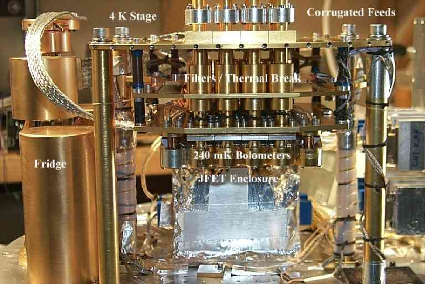
Figure 7: Photo showing the different elements of the Acbar focal plane.

We use the $\sim 100~{}\mu$W of cooling power of the 370 mK intercooler still as a thermal buffer between the 4 K horn plate and the 240 mK detector stage. This intercepts most of the heat load that would otherwise overwhelm the small heat lift of the ultracold stage. There are multiple types of Vespel material and we use SP-1 between 4 K and 370 mK and SP-22 between 370 mK and 240 mK. We estimate the thermal loads from the Vespel legs to be $\sim 40~{}\mu$W on the intercooler stage (370 mK) and $\lesssim 0.1~{}\mu$W on the ultracold stage (240 mK). Figure 7 shows an image of the Acbar focal plane structure along with the sorption fridge.

Flexible thermal straps (see Figure 7) are used to couple the fridge stills to the two thermal stages. These are made from nickel-plated copper braid in which indium is embedded at each end for clamping. The flexible thermal straps reduce the coupling of mechanical resonances of the fridge to the focal plane while providing good thermal conductivity.

All of the isothermal wiring inside Acbar is Teflon-coated gold-plated copper wire and all of the wiring that traverses multiple temperature regions is Teflon-coated stainless wire. Both of these are surgical-quality wires manufactured by Cooner Wire. The stainless wiring is bundled into six twisted pairs within a common stainless shield (corresponding to the six detector channels per bias) with no insulating outer jacket. Stainless wiring has low thermal conductivity but relatively high electrical impedance. All of the wiring for high-current devices (such as resistive heaters) is doubled-up to reduce the power dissipation in the wiring. The wires joining stages at different temperatures are heat sunk at each stage by embedding the wires in a gold-plated copper tab with Stycast epoxy. The stainless wiring is estimated to contribute less than 50 $\mu$W of power on the intercooler stage and around 0.5 $\mu$W on the ultracold stage.

5 Electronics

5.1 Signal Electronics

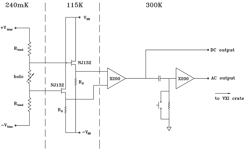
Figure 8: Schematic of the Acbar signal electronics chain. Dashed vertical lines denote thermal boundaries.

The Acbar signal electronics are designed to provide DC bias across the bolometers and read out all channels with low noise from nearly DC to $\sim 100$ Hz. Figure 8 shows a schematic of the Acbar signal electronics chain. The DC bias board supplies a low-noise voltage of 0 to 500 mV symmetrically across the bias resistor stack. There are four bias voltages – one for each row of detectors – which can be set independently and are applied to six detectors each. Two sets of twisted pair stainless wires (one set for redundancy) bring each of the bias voltages to the focal plane where they are broken out to six detectors. In addition to the four optically-loaded bolometers per bias, each of the four biases is also applied to a “dark bolometer” (a bolometer which has been blanked off with a blackened load at 240 mK) and a “fake bolometer” (a 10 M$\Omega$ resistor in place of the bolometer) for use as monitors of base plate thermal drifts, microphonic noise, and amplifier noise.

Each bolometer is in series with two 30 M$\Omega$ metal-film load resistors which were custom made by Mini-systems, Inc.. The load resistor package is surface mounted to a PCB board which is epoxied directly onto the back of the bolometer module. Also mounted on the PCB board is an RFI filter on each side of the bolometer composed of surface-mount 47 nH inductors and 10 pF capacitive feed-through filters which provide filtering above a few hundred MHz directly on the bolometer module.

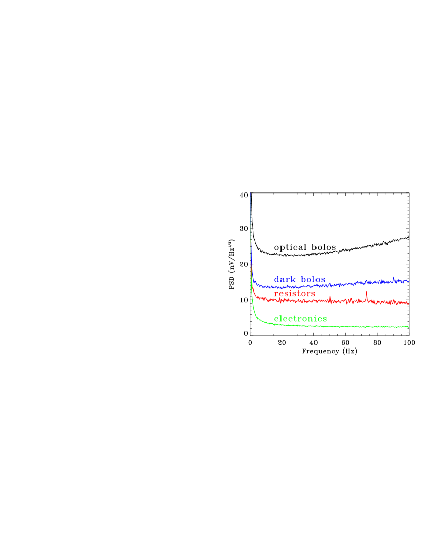
Figure 9: Average voltage noise PSDs of the Acbar signal channels in 2001. The electronics noise (green/bottom) is measured from a pair of JFETs with their gates shorted together and shunted to ground with a 10 k$\Omega$ resistor. The resistor channel (red/second) is for a 10 M$\Omega$ “fake bolometer” mounted on the 240 mK stage. The dark bolometers (blue/third) are blanked off at 240 mK and the optical bolometers (black/top) are the average of all 16 optical channels. A narrow 60 Hz line filter was applied and we corrected for the transfer function of the electronics. As shown in Figure 15, the used signal band is less than 60 Hz and frequencies above the band are removed with a step-function filter. The rise in the optical bolometer noise at high frequency results from correcting for the detector time constants. This is because the Johnson and amplifier noise contributions are not attenuated at high frequency by the detector time constants.

The high impedance ($\sim 7\,{\rm M}\Omega$) of the bolometer signals makes them susceptible to microphonics caused by vibrating wires and RF pickup. In order to reduce these potential sources of noise, pairs of matched JFETs are placed close to the detectors to reduce the output impedance of the signals. The bolometer signal voltages are sent to the JFET modules on twisted pairs of stainless wire. The bolometer signals of a common bias are carried by a shielded bundle of six twisted pairs. Each side of the bolometer voltage is sent into one side of a matched NJ132 JFET source follower pair (see Figure 8). The JFET dies were manufactured by Interfet; they are wire bonded to a single alumina substrate that holds 24 pairs of matched JFETS. These devices have low noise ($\sim 2~{}{\rm nV\,Hz^{-1/2}}$ and an extremely low 1/$f$ knee ($\sim 1~{}{\rm Hz}$); the noise from the JFET followers is small compared to the contributions of the detectors and atmosphere (refer to Figure 9). The dies were probed and selected to form pairs with $<20\,$mV difference in gate-source voltage; this criteria guarantees that the sum of the offset and the detector signal will not saturate the analog to digital converter after applying a gain of 200.

The JFETs cannot operate at 4 K and achieve their lowest noise performance at a temperature of $\sim 115\,$K. The entire JFET module is stood off from the 4 K cold plate with low thermal conductivity G-10 fiberglass legs. A heater is used to raise the temperature of the JFETs to their operating point. In order to minimize the heat load on the helium stage, the heat from the JFET module is intercepted half way down the G-10 legs by a 77 K cold finger that extends from the nitrogen can through the helium can (see Figure 3).

In order to reduce vibrations of the high impedance wiring connecting the detectors and JFETs, the JFET module and detector array are both secured with a tensioned Kevlar support harness. The Kevlar strands are tensioned with spring washers to overcome the negative coefficient of thermal expansion of Kevlar. The addition of this harness pushes the vibrational resonance frequencies of the focal plane and JFET module well above the signal band.

RFI entering the 4 K vacuum space can couple to the high impedance wiring on the focal plane; this can heat the detectors and degrade their sensitivity or introduce noise to the signals. All wires entering the 4 K vacuum space pass through additional RFI filter modules mounted in the wall of the liquid helium radiation shield. The filters used in these modules are muRata EMI $\pi$-filters which have been embedded, along with the wires from the connectors, in castable Eccosorb. These RFI filter modules were measured to attenuate signals above 1 GHz better than -60 dB (Leong 2001).

The signal wires exit the dewar through hermetic connectors and enter the warm electronics signal box where they are filtered and amplified. The electronics boxes are mounted directly on the cryostat. The boxes have RF shielding gaskets at all mating surfaces. The raw signals are low-pass filtered at $650\,$Hz and amplified by a factor of 200. The DC offset is removed with a low-pass filter at $\sim 16$ mHz ($10\,$s time constant). In order to avoid a long wait for the readout to settle after a change in elevation, a MOSFET switch is used to momentarily short the capacitor in the low-pass filter and remove the DC offset. The AC signals are amplified by another factor of 200 (for a total gain of 40,000). The total noise contribution from the JFETs and warm electronics is $<10~{}{\rm nV\,Hz^{-1/2}}$ for $\nu>2$ Hz with a white noise level of $\sim 3~{}{\rm nV\,Hz^{-1/2}}$ for $\nu>10$ Hz. Figure 9 shows the voltage noise of the electronics, resistor channels, dark bolometers, and optically loaded bolometers. The electronics noise contributes a small fraction of the total noise of the optically loaded detectors over most of the signal bandwidth.

The signals are then low-pass filtered at 650 Hz and sent to an Agilent Technologies VXI data acquisition system housed in a heated enclosure on the back of the telescope primary mirror. There the signals are anti-alias filtered by a 1-pole filter with 3dB point at $100\,$Hz, sampled with 16-bit resolution at $2400\,$Hz, and averaged over 8 samples to reduce the data rate. The averaging puts the Nyquist frequency at 150 Hz and does not effect our signal bandwidth. We transfer the data to the U.S. using the TDRSS satellite network. This allows the local science team to monitor the state of the instrument and analyze data within a day of acquisition.

5.2 Transfer Function

Modulated optical signals undergo a considerable amount of filtering between absorption by the detectors and the digitized voltages written to disk. The transfer function of the system quantifies the amplitude attenuation and phase shift of modulated optical signals as a function of modulation frequency. The filter components of the Acbar transfer function are single-pole detector time constants, $RC$ filter from detector impedance and capacitance from wiring and JFETs, 650 Hz low-pass $RC$ filter, 100 Hz single-pole anti-aliasing filter in the A/D, and a sinc filter from the box-car averaging of 8 samples. We measure the complete transfer function by varying the frequency of a small, chopped, thermal source from 5 to 200 Hz and record the amplitude and phase of the output signal. The time-stream data for each optical channel is corrected for the complete transfer function with the appropriate detector time constants.

5.3 Computer Control and Housekeeping

Acbar can be configured for either manual or computer control of all system elements by flipping large toggle switches (for ease of use with gloved hands) on the electronics boxes. Under manual control, all receiver settings can be made with turn pots. Under computer control the settings are changed with a digital bus. The digital bus allows remote setting of all of the following: bolometer bias levels, all heaters on fridge and cold stages, calibrator temperature and modulation frequency, and all thermometer settings (reference impedance and excitation voltage). This allows the observer to control virtually all aspects of the instrument from within the main station dome, located approximately 1 km away from the telescope. All of the housekeeping information is read by the A/D at 2 Hz and saved to disk. This includes all bias levels, thermometry readings, DC levels of all 24 detectors, and the two-axis tilt meter mounted on the telescope.

6 Observations

6.1 Beam Sizes

Accurate measurement of the beam sizes on the sky is important for calibrating the instrument and generating CMB window functions. The planets Mars and Venus are our objects of choice for measuring beam sizes. The beam solid angle is determined by integrating the source voltage over raster maps (that have been flat-fielded) and dividing by the source amplitude. The measured beam sizes from Mars on 2001 July 17 and Venus on 2002 September 22 are listed in Table 4.

The beam sizes for the 150 and 350 GHz channels differ from the nominal $4^{\prime}$ Gaussian FWHM. The 150 GHz beams are diffracted by the aggressive edge taper (-18dB) on the 2 m primary mirror and the $\sim 20\%$ increase in size agrees with the level predicted for a truncated Gaussian (Goldsmith 1998). The 350 GHz beams are properly sized exiting the cryostat and are not improved by focusing the telescope; the large beams sizes are most likely the result of telescope surface roughness.

The beam size varies within a frequency column/row, indicating some aberration across the focal surface. We chose the dewar focus position that, on average, resulted in the minimum beam size from galactic source raster maps. We made a particular effort to minimize the beam size of the 150 GHz channels because they are the most sensitive for CMB and SZ observations.

The beam sizes change slightly with chopper angle, indicating that the beams are distorted as the chopper rotation changes the optical path through the telescope. The effect was measured to be $\sim 5\%$ in 2001 but was reduced by about a factor two in 2002 with an improved alignment of the optics. The changing beam sizes also affect the CMB window functions of the instrument. This effect is discussed in detail in Kuo et al. (2002). The conservation of optical throughput with chopper angle was tested by making complete raster maps of galactic sources at multiple chopper offset positions and integrating the maps over solid angle. We used the compact HII region MAT6a (Puchalla et al. 2002) for this measurement because of the limited availability of planets and bright point sources. The integrated source voltage of MAT6a versus chopper position is found to be flat, indicating good conservation of optical throughput.

In late September 2002 we noticed that ice crystals had accumulated on the foam dewar window and removed them. From maps of Venus before and after the ice removal, we discovered a significant change in some of the beams. The ice on the curved surface of the window acted like a thin lens, distorting the focal plane. The average FWHM beam sizes before the ice removal were $4.89^{\prime}$, $4.30^{\prime}$, and $4.23^{\prime}$ at 150, 220, and 280 GHz, respectively. After the ice removal, the average beams measured $4.69^{\prime}$, $4.25^{\prime}$, and $3.95^{\prime}$. In addition, the positions of some of the beams were shifted by a substantial fraction of an arcminute on the sky. Both of these effects tend to smear the effective beam size of the coadded maps. Fortunately, we included a bright point source in our CMB fields (see §6.6) and observed galactic sources multiple times per day; these allow us to measure changes in the position and size of each beam and correct for the effects of ice accumulation over time.

6.2 Chopper Synchronous Offsets

When the chopper is running, the bolometer signals are dominated by a chopper synchronous offset that is well described by a second-order polynomial. The chop across the sky is roughly constant latitude at $45^{\circ}$ elevation and we would expect an offset from motion of the beams through the atmosphere at different elevations. The amplitude of the temperature offset due to motion through the atmosphere is approximately equal to

$$\Delta T\sim 2.6~{}{\rm mK}\left({\frac{T_{sky}}{220~{}{\rm K}}}\right)\left({\frac{\tau}{0.03}}\right)\left({\frac{\Delta}{1^{\prime}}}\right)$$ (3)

where $T_{sky}$ is the temperature of the atmosphere, $\tau$ is the atmospheric opacity, and $\Delta$ is the elevation change from the curvature of the chop. However, the observed temperature change is at times much larger than the predicted amplitude from the atmosphere, and sometimes has the opposite sign. This indicates the offset is often dominated by effects other than the changing elevation of the beams through a smooth atmosphere.

The offset structure is observed to depend on a number of factors. Modulated chopper spillover, accumulation of snow on the telescope, and atmospheric conditions appear to be the dominant contributors to offset amplitude. The first two sources are within our ability to control and we take steps to mitigate their effects. We reduced modulated mirror spillover by mounting a blackened circular light baffle between the tertiary mirror and the chopper. This light baffle is somewhat smaller than the projected area of the chopper and intercepts beam power which would otherwise spill over and modulate as the chopper rotates. The baffle significantly reduced the offset amplitude of the chopper offset. As discussed below in §6.4, this warm baffle contributes to the loading of the system because it intercepts beam power at ambient temperature.

6.3 Snow

Snow accumulation is another large contributor to the chopper synchronous offsets. The mirror surfaces collect blowing snow as well as develop a thin layer of frost over time. As the chopper rotates, the detector beams view different projections of the chopper mirror and are swept across the secondary mirror. The chopper is placed at an image of the primary, so the illumination of the primary mirror is approximately constant. Unevenly distributed snow on the chopper and secondary mirrors contributes an optical signal (or “chopper offset”) through emission and scattering. To avoid this, we clean and defrost the mirrors frequently.

In addition to contributing to offset structure, snow accumulation also attenuates astronomical signals. The method of signal loss is likely to be a combination of absorption and scattering by crystals with size comparable to $\lambda$. This signal attenuation was discovered by comparing the measured amplitude of galactic sources versus chopper offset amplitude. To test the effects of snow on signal attenuation we performed raster maps of the galactic source RCW38 with the mirrors very snowy and then repeated the observation with the mirrors cleaned. The average signal ratios for RCW38 with the mirrors snowy versus clean were 70%, 45%, and 20% at 150, 220, and 280 GHz, respectively, indicating a strong frequency dependence of the signal loss. The beam solid angles are effectively unchanged between the snowy versus clean measurements, which indicates that any scattering would have to be relatively isotropic to explain the signal loss without an appreciable broadening of the beams. We minimize the effects of snow accumulation by identifying periods when the data may be contaminated from snow and discarding them.

To develop a criteria for cutting data with snow contamination, we investigated the correlation of chopper offset amplitude with integrated source signal and found a strong correlation at high frequency and a weaker correlation at low frequency. This frequency dependence allows us to tune the level of tolerable snow attenuation to the science goal being investigated. For example, the weaker dependence at 150 GHz means that a more aggressive snow cut threshold (fewer files removed) can be used for science only incorporating the low-frequency channels. However, pointed cluster observations rely on the high-frequency data to remove the CMB contribution from the maps and must therefore employ a more conservative snow cut threshold (more files removed) to prevent severe signal attenuation at the higher frequencies.

6.4 Optical Loading

The optical loading on all channels can be determined at any time from the DC voltage levels of the bolometers and the detector cold plate temperature using the measured properties of the bolometers. The average RJ loading temperature for 2002 at all three frequencies is listed in Table 5. The variation in optical loading is found to correlate well with atmospheric opacity.

The dominant sources of loading for Acbar are warm filter optics, atmosphere, and a warm telescope. We took great pains to reduce the internal optical loading from the dewar by maximizing the in-band transmission of the warm filters and blocking high-frequency leaks at cold temperatures. The atmospheric contribution is given by $T_{atm}=T_{sky}(1-e^{-\tau/\cos\zeta})$ where $T_{sky}$ is the physical temperature of the atmosphere, $\tau$ is the average in-band zenith opacity, and $\zeta$ is the zenith angle of the observation. On a typical day, the temperature loading from the atmosphere at $EL=60^{\circ}$ is 8, 13, and 24 K at 150, 220 and 280 GHz, respectively. The telescope consists of four warm aluminum mirrors, each of which has a theoretical emissivity of a fraction of a percent from Ohmic loss. The actual emissivity of the surface is greater than this value because of reduced conductivity from surface roughness. Surface roughness also contributes to loading through Ruze scattering onto warm surfaces. The introduction of a light baffle to reduce chopper synchronous offsets also contributes to the optical loading. The large beams of the 150 GHz channels are truncated at the baffle aperture at a level which contributes $\sim 5$ K, but the beams from the higher frequencies are sufficiently small that the baffle contribution is $\lesssim 1$ K. The average total RJ loading on the bolometers at $60^{\circ}$ elevation in 2002 (and associated $1\sigma$ dispersion) was $39\pm 6$ K at 150 GHz, $37\pm 10$ K at 220 GHz, and $65\pm 15$ K at 280 GHz. The variation in loading is highly correlated with changes in atmospheric opacity.

6.5 Scan Strategy

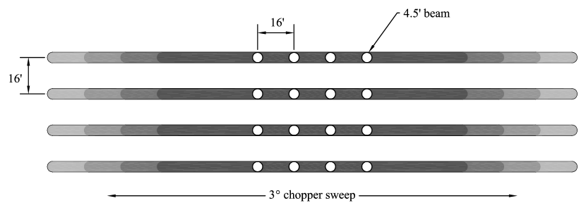
Figure 10: Illustrates the sky coverage geometry of a single declination “stare.” The 16 pixels are swept $\sim 3^{\circ}$ on the sky and the darkness of the shading indicates the degree of overlap of the four channels within each row. Full raster maps are built up by tipping the telescope down $1^{\prime}$ in elevation and repeating this process approximately 100 times.

We perform elevation raster maps when observing the CMB with Acbar. We track a fixed RA-DEC position with the chopper running for 30 to 60 seconds; this is referred to as a “stare.” We then tip the telescope down $1^{\prime}$ in elevation and repeat the process. We perform $\sim 100$ elevation steps which results in a large patch of sky sampled by all four rows of the focal plane. The sky coverage of the array during a single stare is illustrated in Figure 10.

As described above, the dominant signal in the raw raster maps is a roughly parabolic signal a few mK in amplitude. The chopper synchronous offset signals change with time and we were concerned that changing small-scale variations in the offset signal could contaminate the maps. We devised an observing strategy to remove as much chopper synchronous offset as possible – even if slowly time varying – while preserving the large-scale CMB power in the map.

We employ a LEAD-MAIN-TRAIL (LMT) observing strategy in which we raster three $\sim 3^{\circ}\sec\delta$ wide fields that almost touch in RA. The raster progresses by observing the three fields in succession at fixed elevation before proceeding to the next elevation. The fields are usually observed for 30 seconds on LEAD, 60 seconds on MAIN, and 30 seconds on TRAIL. If the offset is constant or changing linearly with time, then the average offset of the LEAD and TRAIL fields should equal the offset in MAIN. By forming the difference $LMT=M-(L+T)/2$, we eliminate both constant and linearly drifting offsets. We also divide the observations into $A$ and $B$ halves which are shifted by $\sim 0.5^{\circ}\sec\delta$ in RA. This shift provides an additional test of systemic effects.

The three fields are separated by about $3^{\circ}$ on the sky, which is larger than the $\sim 1^{\circ}$ peak correlation of the CMB; thus the $LMT$ subtraction should not remove much CMB power. In fact, if the CMB fluctuations are random and uncorrelated, then the $LMT$ map should have $\sqrt{3/2}$ times the CMB signal of the MAIN field alone. When searching for SZ clusters, we are not concerned with preserving the large-scale CMB power in the maps. We can treat the three $LMT$ fields as separate and remove an average offset plus higher order polynomial to eliminate the chopper synchronous signal; this preserves the unique frequency spectrum of the thermal SZ effect so that clusters will always appear as decrements at 150 GHz in the three separate fields. This is discussed in more detail in Runyan et al. (2003).

6.6 Field Selection

When selecting fields for deep CMB observations at millimeter wavelengths, the primary foreground contaminant of concern is dust emission (Tegmark & Efstathiou 1996). Most of the Southern celestial hemisphere is available for continuous observation and we select regions of very low dust contrast for our observations. The IRAS/DIRBE dust map of Finkbeiner et al. (1999) provides a template of galactic dust emission with the best region of the Southern Hemisphere lying roughly between $21^{h}$ to $5^{h}$ in RA and $-20^{\circ}$ to $-70^{\circ}$ in DEC.

With thousands of square degrees of clean sky available, we decided to center the fields on millimeter-bright point sources. These sources provide a continuous monitor of pointing during CMB observations, as well as a bright point source for measuring the final beam size in the coadded maps. The coadded point source image incorporates the physical extent of the beams as well as beam smearing due to pointing jitter. We surveyed many of the flat-spectrum radio sources in the Southern Hemisphere observed by SEST (Beasley et al. 1997; Tornikoski et al. 1996, 2000) searching for candidates bright enough to detect with high S/N in a single raster map. The sources selected for the CMB fields observed by Acbar in 2001 and 2002 are listed in Table 6.

6.7 Data Cuts

We apply a variety of cuts to the raw data set before inclusion in the coadded maps. Our total observing efficiency during the winter of 2002, including galactic source observations and calibrations, was $\sim 60\%$ before any data cuts were applied. The first data cut is based on the reliability of the pointing solution for a given observation. There are brief periods of time where the observation of galactic sources does not yield a consistent pointing solution and observations during these periods are excluded. We next verify that the ³He refrigerator base temperature is cold ($<$ 250 mK) during the entire observation to prevent significant changes in detector responsivity; if the refrigerator is still cooling down or warming up during an observation, we do not include that data. We also cut an entire chopper sweep for a channel with a detectable cosmic ray spike above $5\sigma$.

Our final data cut is referred to as the “snow cut.” As mentioned above in §6.3, accumulation of snow on the telescope mirrors causes a chopper synchronous signal and attenuates astrophysical signals before they reach the detectors. The magnitude of signal attenuation depends strongly upon frequency and the snow cut threshold can be relaxed for an analysis incorporating only the low-frequency data. Figure 11 shows a histogram of chopper synchronous offset RMS during observations of the CMB5 field. The snow cut employed for the analysis of the 150 GHz CMB power spectrum presented in Kuo et al. (2002) corresponds to a chopper offset RMS of 20 mV. This cut level limits the signal attenuation from snow to $\lesssim 5\%$ at 150 GHz and removed $\sim 40\%$ of the raw data. There is a high degree of correlation between the data corrupted by snow accumulation and the data with increased atmospheric correlation. This indicates that rapid snow accumulation is associated with poor atmospheric observing conditions.

7 Calibration

7.1 Planetary Observations

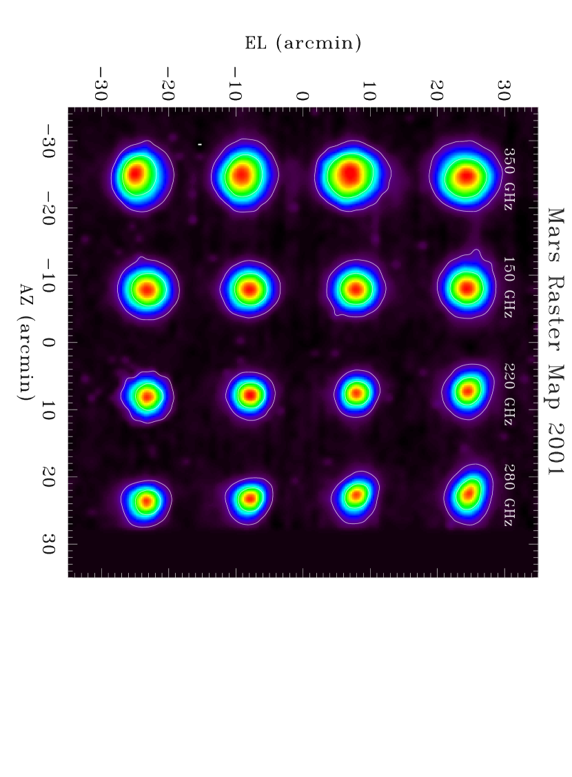
Figure 12: Raster map of Mars at an elevation of $26.5^{\circ}$ taken on 2001 July 16. The angular diameter of Mars was $19^{\prime\prime}$ on this date and the map has been smoothed with a $1^{\prime}$ FWHM Gaussian. The white contours correspond to power levels of 10% and 50%.

To convert measured signal voltages to physically meaningful units, we observe an object of known flux. Our primary calibration source for the 2001 season was the planet Mars, which has been well studied at millimeter wavelengths (Griffin et al. 1986). We observed Mars multiple times during the year in an effort to develop a consistent calibration and check for systematic effects. For the 2002 season, we used the planet Venus as our primary calibrator. Venus was only visible above the horizon at the end of the 2002 season. Much less is known about Venus at millimeter wavelengths and its complicated atmosphere makes the uncertainty of its brightness temperature quite high ($\sim 8\%$ at 150 GHz) (Ulich 1981). Raster maps of Mars and Venus used to calibrate the instrument are shown in Figures 12 and 2.

We determine the flux of Mars during an observation using the FLUXES software package developed for the JCMT telescope on Mauna Kea. FLUXES provides the brightness temperature of some of the planets on any date across a range of millimeter and sub-millimeter wavelengths. FLUXES incorporates a model to correct the Martian brightness temperature with varying Sun-Mars distance. For Venus, we use the table of published brightness temperatures listed in Weisstein (1996). We determine the position and solid angle, $\Omega_{P}$, of the planets from the online NASA planetary ephemeris (Espenak 1996). Typical brightness temperatures for Mars were $\sim 208$ K at 150 GHz during our CMB observations in 2001 with a reported error of $5\%$. The brightness temperature of Venus is approximately 294 K at 150 GHz (Ulich 1981) with an error of 8%. The planetary brightness temperatures as a function of frequency, $T_{B}(\nu)$, are well fit by a straight line between 100 and 400 GHz. For each planetary observation, we convolve this linear fit with the frequency response of our detectors, $f(\nu)$, to determine the band-average planetary flux density for each channel

$$\bar{S}_{P}=\frac{\int 2kT_{B}(\nu)(\nu/c)^{2}\Omega_{P}f(\nu)d\nu}{\int f(\nu)\,d\nu}.$$ (4)

However, we observe the planet through an attenuating atmosphere and must correct for the atmospheric opacity to determine the actual planetary flux arriving at the instrument.

7.2 Atmospheric Opacity

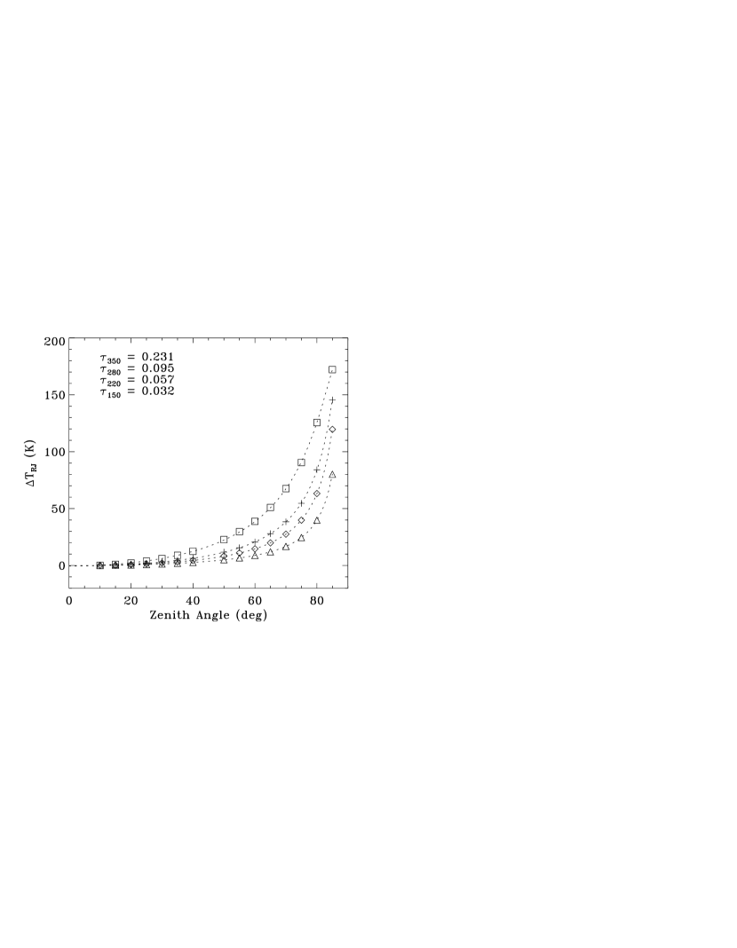
Figure 13: Skydip performed on 2001 February 13 when the 350 $\mu$m zenith opacity was measured to be 1.77. The figure shows the change in sky temperature from the zenith (averaged over the four channels at each frequency) versus zenith angle ($\zeta$). The four sets of points are 350 (squares), 280 (pluses), 220 (diamonds) and 150 GHz (triangles) and the dotted lines are analytic fits to $\Delta T_{RJ}(\zeta)=T_{atm}\left({e^{-\tau}-e^{-\tau/\cos\zeta}}\right)$.

To determine to actual planetary flux incident on our detectors – as well as astrophysical source flux during normal observations – we need to characterize the transmission of the atmosphere. We perform sky dips to determine the atmospheric zenith opacity for each channel, $\tau$ (see Figure 13). Typical measured values of zenith opacity are 0.033, 0.052, 0.10, and 0.18 at 150, 220, 280, and 350 GHz, respectively.

Because sky dips are a time consuming process, we developed a method which avoids having to perform sky dips regularly but still permits frequent monitoring of the atmospheric transmission. We determined the relationship between the measured in-band opacities for Acbar and a 350 $\mu$m tipper experiment located on the adjacent AST/RO building (Radford 2002) which measures the sub-millimeter opacity of the South Pole atmosphere approximately every 15 minutes. We performed many sky dips during both observing seasons and correlated the measured in-band zenith opacities with those measured by the 350 $\mu$m tipper; the relationship is very linear.

7.3 Detector Responsivity

We also correct for the change in detector responsivity due to the different optical loadings at low elevation for planets and high elevation for CMB and cluster observations. After each planetary observation, we run the small calibrator source mounted behind a hole in the tertiary at 5 Hz. The chopped source provides a reference signal at planetary elevations for each channel, $V^{cal}_{P}$, that is used to scale the bolometer responsivity for future observations. To correct the change in bolometer responsivity with elevation, we run the chopped calibrator source again at the elevation of the CMB observations and divide the responsivity by the measured ratio of the observation calibrator voltage, $V^{cal}_{obs}$, to the planetary calibrator voltage. The slow chop frequency makes the measured calibrator signal insensitive to any changes in detector time constants with loading.

Because of the gradual accumulation of snow around the hole in the tertiary, this responsivity transfer is only useful for observations spaced closely in time. However, after the snow cut, the measured signal from the galactic source RCW38 has an RMS scatter of $<4\%$ which is largely due to residual signal attenuation from the snow. This also demonstrates that the detector responsivity at high elevation is quite stable. The calibration for each observation is then

$$R=\frac{\bar{S}_{P}}{\int V_{P}(\Omega)\,d\Omega}\frac{e^{-\tau_{P}/cos(\zeta_{P})}}{e^{-\tau_{obs}/cos(\zeta_{obs})}}\frac{V^{cal}_{P}}{V^{cal}_{obs}}\qquad\text{[Jy V${}^{-1}$sr${}^{-1}$]},$$ (5)

where $\int V_{P}(\Omega)\,d\Omega$ is the integral of the planetary voltage map over the sky and $\tau$ and $\zeta$ are the atmospheric opacity and zenith angle of the observation, respectively.

Observations of the cosmic microwave background are usually calibrated into CMB temperature units. Because we measure fluctuations in the CMB (rather than total power) the conversion between flux density and temperature is given by

$$\Delta S=\frac{dB_{\nu}}{dT}\Omega_{B}\Delta T,$$ (6)

where $B_{\nu}$ is the black body spectral energy density and $dB_{\nu}/dT$ is evaluated at $T_{CMB}$. The desired calibration from signal voltage to CMB temperature units is given by

$$R^{CMB}=R\left[{\frac{\int\frac{dB_{\nu}}{dT}f(\nu)\,d\nu}{\int f(\nu)\,d\nu}}\right]^{-1}\qquad\text{[K V${}^{-1}$]},$$ (7)

where we have averaged the conversion from flux density to Kelvin over the frequency band. We estimate the total $1\sigma$ uncertainty in the calibration for 2001 and 2002 to be $\pm 10\%$.

The breakdown of contributions to the 2002 calibration uncertainty at 150 GHz is $8\%$ from the brightness temperature of Venus, $2\%$ from the residual RMS in the planetary voltage map integral, $2\%$ from calibrator responsivity scaling, and $<1\%$ from the transmission of the atmosphere. As discussed in the following section, we cross-calibrated the galactic source RCW38 in 2001 and 2002 to check for systematic effects. We include an additional calibration uncertainty of $3\%$ from the scatter in cross-calibrated RCW38 flux from Venus at 150 GHz and $3\%$ systematic uncertainty from the consistency of the RCW38 calibration between 2001 and 2002. Table 8 includes a list of potential systematics and their contribution to the calibration uncertainty at 150 GHz.

7.4 Galactic Source Cross-Calibration

During the 2002 observing season, there were no bright planets available until September 2002. To monitor the calibration during the year, we use the frequent galactic source observations and cross-calibrate the galactic sources with a planet. We determine the band-averaged integrated flux density of an object, $S_{2}$, from an object of known flux density, $S_{1}$, by

$$S_{2}=S_{1}\frac{\int V_{2}d\Omega}{\int V_{1}d\Omega}\frac{V_{1}^{cal}e^{-\tau_{1}/\cos\zeta_{1}}}{V_{2}^{cal}e^{-\tau_{2}/\cos\zeta_{2}}},$$ (8)

where the ratio $(V_{1}^{cal}e^{-\tau_{1}/\cos\zeta_{1}})/(V_{2}^{cal}e^{-\tau_{2}/\cos\zeta_{2}})$ accounts for the change in atmospheric transmission and bolometer responsivity between the two observations.

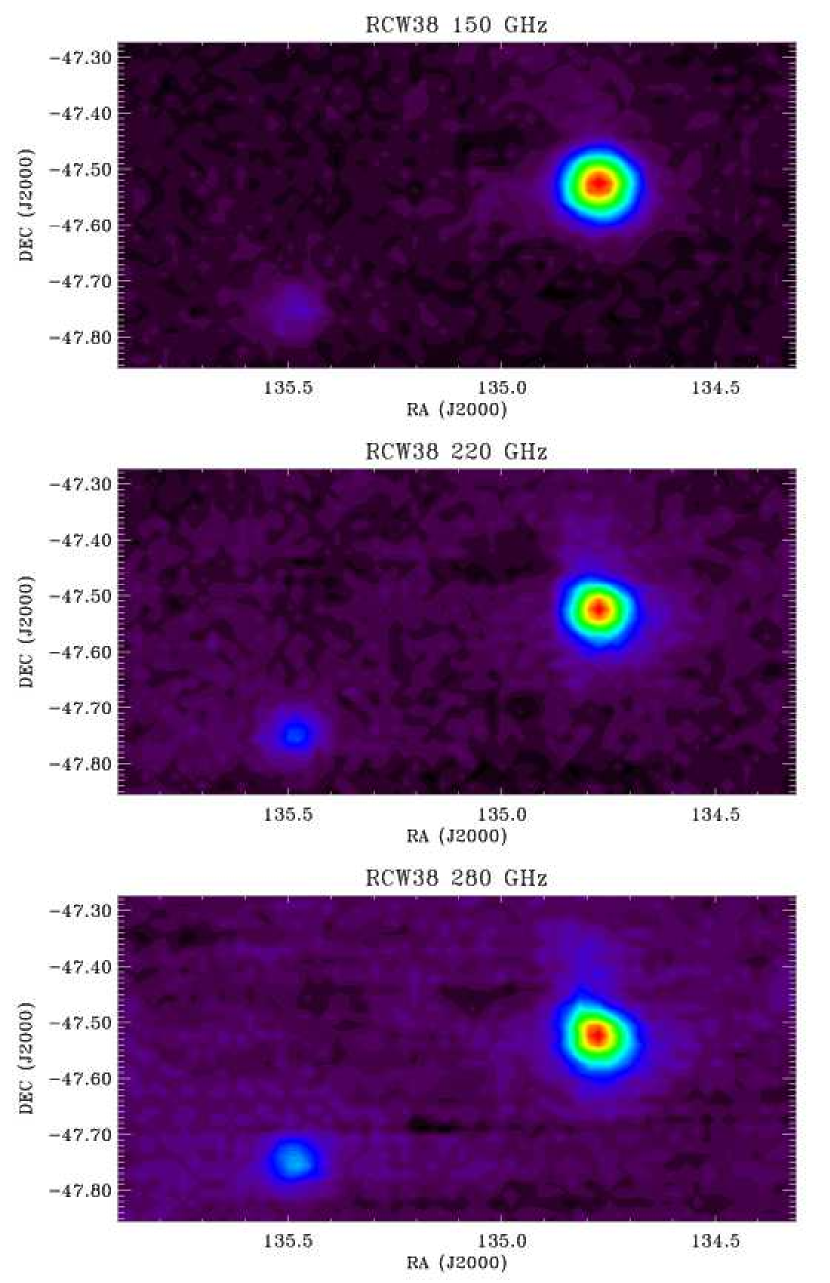
Figure 14: Single-channel raster maps of RCW38 taken on 2001 June 9. The signal-to-noise on the source is very high in a single raster map. We use RCW38 to monitor both the telescope pointing and instrument calibration. The source in the lower-left corner of the maps appears to be associated with IRAS 09002-4732.

We apply this method to RCW38 in both 2001 and 2002 with Mars and Venus, respectively. We used RCW38 and planetary observations taken within one day of each other and insist that both observations have calibrator runs for scaling the detector responsivity. We integrate the flux within $8^{\prime}$ of the source center; these results are given in Table 7. The agreement between the integrated flux is good at 150 and 280 GHz but the 220 GHz observations in 2001 suffer from low number statistics. A raster map of RCW38 taken on 2001 June 9 is shown in Figure 14. The complex extended structure of RCW38 – particularly at 220 and 280 GHz – is apparent even in a single raster image.

8 Noise and Sensitivity

There are multiple sources that contribute to noise in the Acbar instrument (Richards 1994; Mather 1984) but the instrument is fundamentally limited by the random arrival of background photons. Characteristics that determine whether the system will be background limited are: optical power incident on a detector, bandwidth of observed light, optical efficiency, detector impedance, detector thermal conductivity, operating temperature, electronics noise, as well as the atmospheric conditions of the site (Griffin & Holland 1988). The complete noise budget for Acbar in 2002 is presented in Table 5; we have included estimates of the noise contributions from the photon background ($NEP_{\gamma}$), Johnson noise ($NEP_{J}$), phonon noise ($NEP_{G}$), and amplifier noise ($NEP_{A}$). Refer to Richards (1994) and Mather (1984) for details on the calculation of noise contributions in bolometric systems. We have included expected contributions from both the counting and photon bunching in $NEP_{\gamma}$ in our estimated noise table. See Appendix B for a discussion on the inclusion of photon bunching.

The average total $NET_{RJ}$ between 10 and 20 Hz (above the $1/f$ knee from the electronics and atmosphere but well within the signal band) for 2002 were 200, 250, and 280 $\mu{\rm K}\sqrt{\rm s}$ at 150, 220, and 280 GHz, respectively. For comparison, the $NET_{RJ}$ on a very good day in 2001 were 340, 380, 270, and 950 $\mu{\rm K}\sqrt{\rm s}$ at 150, 220, 280, and 350 GHz, respectively. The substantial improvement at the lower frequencies resulted from a filter upgrade in December 2001. When combined with the addition of a second row of 150 GHz channels (replacing the 350 GHz detectors), the upgrade resulted in a nearly six-fold improvement in 150 GHz mapping speed. A plot of the average $NET_{CMB}$ versus frequency for the 150 GHz channels in 2002 is shown in Figure 15.

9 Conclusions

We have described the design and performance of the Arcminute Cosmology Bolometer Array Receiver (Acbar). We have taken advantage of improvements in bolometric detector technology and the superb observing conditions afforded by the South Pole to make very sensitive, high resolution maps of the CMB at multiple millimeter wavelengths. Acbar was installed on the Viper telescope in January 2001 and has mapped the microwave sky through November 2002. The instrument is background photon limited at all frequencies, with an average $NET_{CMB}$ per detector of $350~{}\mu{\rm K}\sqrt{\rm s}$ at 150 GHz, and the measured noise level is more consistent with the noise model if we include the photon bunching contribution.

The CMB power spectrum measurement from a subset of Acbar’s 2001 and 2002 data is presented in Kuo et al. (2002) and the constraints on cosmological parameters derived from this power spectrum are given in Goldstein et al. (2002). We have searched within these maps for SZ clusters of galaxies (Runyan et al. 2003) to constrain models of structure formation. As part of a multi-wavelength investigation of nearby cluster physics, we have also surveyed a fluxed-limited sample of clusters at $z<0.1$ with sufficient sensitivity at multiple frequencies to separate the primary CMB and thermal SZ emission (Gomez et al. 2002).

We acknowledge assistance in the fabrication of Acbar by the capable staff of the U.C. Berkeley, U.C. Santa Barbara, and Caltech machine shops and the U.C. Berkeley electronics shop. The support of Center for Astrophysics Research in Antarctica (CARA) polar operations has been essential in the installation and operation of the telescope. We would like to thank John Carlstrom and Steve Meyer for their early and continued support of the project. We gratefully acknowledge Simon Radford for providing the 350 $\mu$m tipper data. We thank Charlie Kaminski and Michael Whitehead for their assistance with winter observations. This work has been primarily supported by NSF Office of Polar Programs grants OPP-8920223 and OPP-0091840. Marcus Runyan acknowledges many useful discussions with B. P. Crill, S. Golwala, W. C. Jones, P. D. Mauskopf, and B. J. Philhour, help with lab measurements by Dan Marrone, and the support of a NASA Graduate Student Researchers Program fellowship. Chao-Lin Kuo acknowledges support from a Dr. and Mrs. CY Soong fellowship. We also thank the referee for useful suggestions on the manuscript.

Appendix A Bandwidth and Optical Efficiency

In this appendix we discuss the subjects of system bandwidth and optical efficiency. Traditionally, the optical bandwidth of a system is defined as the full-width at half the maximum transmission of a measured frequency spectrum. Although this number is quantitative in the sense that it can be measured precisely from any given spectrum, it does depend intrinsically upon the resolution of the spectrum from which it is calculated. For example, fringes in a high-resolution spectrum will tend to push the “half-maximum” point further up the band compared to a smooth low-resolution spectrum from the same optical system.

Consider an optical system with measured spectral response, $f(\nu)$. This spectrum is normalized by measuring the multiplicative optical efficiency coefficient, $\eta$, such that the optical power, $Q$, measured from a beam-filling source of spectral intensity, $I(\nu)$, is given by

$$Q=\eta\int f(\nu)I(\nu)A(\nu)\Omega(\nu)d\nu,$$ (A1)

where $A(\nu)\Omega(\nu)$ is the frequency-dependent optical throughput of the system; $A\Omega=\lambda^{2}$ in the case of a single-moded system. We define the efficiency normalized spectral response as $\tilde{f}(\nu)=\eta f(\nu)$. In the case of a RJ emitting source at temperature $T$, the spectral intensity is given by $I(\nu)=2kT\nu^{2}/c^{2}$ and the optical power absorbed by the detector in a single-moded system is $Q=2kT\int\tilde{f}(\nu)d\nu$.

We would like to identify the quantities bandwidth, $\Delta\nu$, and average optical efficiency, $\bar{\eta}$, such that $Q=2NkT\bar{\eta}\Delta\nu$, where $N$ is the number of optical modes supported by the system. Limiting ourselves to the case of a single optical mode ($N=1$) this leads to the relation $\int\tilde{f}(\nu)=\bar{\eta}\Delta\nu$. The key point is that the average optical efficiency and effective bandwidth are not separable quantities. As long as the bandwidth is clearly defined, then the average optical efficiency is given by $\bar{\eta}=\Delta\nu^{-1}\int\tilde{f}(\nu)d\nu$. Although the width of the band at half maximum will give a ball park measurement of the bandwidth, we would like to use a bandwidth estimator that is robust to changes in the resolution of the spectrum.

The derivative of a transmission spectrum with frequency, $\tilde{f}^{\prime}=d\tilde{f}/d\nu$, emphasizes those regions of the spectrum where the band is changing significantly – it has a large positive value when the band is rising and a large negative value when the band is falling. Using the derivative of the band as a weight, we can determine the edges of the band. High-resolution spectra will result in fringing in the derivative but these fringes will average out.

Consider an arbitrarily normalized transmission spectrum, $f(\nu)$, with band center $\nu_{0}=\frac{\int\nu f(\nu)d\nu}{\int f(\nu)d\nu}$ and frequency derivative, $f^{\prime}(\nu)$. We identify the lower and upper band edges as

$$\nu_{L}=\frac{\int_{0}^{\nu_{0}}\nu f^{\prime}(\nu)d\nu}{\int_{0}^{\nu_{0}}f^{\prime}(\nu)d\nu},\quad\nu_{U}=\frac{\int_{\nu_{0}}^{\infty}\nu f^{\prime}(\nu)d\nu}{\int_{\nu_{0}}^{\infty}f^{\prime}(\nu)d\nu}.$$ (A2)

The bandwidth is then defined as $\Delta\nu=\nu_{U}-\nu_{L}$. This bandwidth estimator depends only weakly upon the exact value of $\nu_{0}$ used in the integrals for reasonably contiguous bands (eg. bands with only have one main “lobe”).

To see that this definition of bandwidth is sensible, consider the two cases of a top-hat and Gaussian band. In the case of the top-hat band, the derivatives become delta functions at the band edges and the result is straight forward. For the Gaussian case, the band does not have well defined “edges” and the derivative will have maxima and minima at the inflection points of the Gaussian. Even for a Gaussian band with much non-localized transmission, calculating the bandwidth with the equations above results in a bandwidth a few percent larger than the FWHM of the band.

Real-world bands are not so nicely behaved as the two examples above. In Figure 16 we show the average of the Acbar 150 GHz bands as well as its derivative. We show both the raw derivative as well as a smoothed derivative to show where the derivative will weight the band edges most heavily. Because the frequency, $\nu$, is a smoothly varying function, the rapid variations in the derivative are averaged out in the integral. This method was used to calculate the bandwidths and average optical efficiencies presented in this paper and should yield normalization and resolution independent measures of bandwidth for well behaved spectral bands (eg. bands that do not have bulk features such as a large gouge in the middle of the band).

Appendix B Photon Noise

Photon noise is the result of temporal fluctuations in the rate of photon arrival at the detectors. A series of pioneering papers by Hanbury Brown & Twiss (1957, 1958a, 1958b) showed that in addition to the Poisson counting noise, there is a bunched component due to the Bose statistics describing the photons. The same authors also showed that if the detection bandwidth is much smaller than the optical bandwidth ($30$ Hz vs. $30$ GHz for Acbar), both noise components have a white power spectrum (Hanbury Brown & Twiss 1957).

Following the derivation given in Appendix A of Hanbury Brown & Twiss (1958a), Lamarre (1986) finds an expression for the noise equivalent power ($NEP$) of the fluctuations in optical power;

$$NEP^{2}=\left[2\int h\nu Q_{\nu}d\nu+(1+\!P^{2})\int{\mathcal{D}}_{\nu}Q_{\nu}^{2}d\nu\right]\qquad\left[\rm W^{2}Hz^{-1}\right],$$ (B1)

where $P$ is the degree of polarization, $Q_{\nu}$ is the specific flux (${\rm WHz^{-1}}$), and the partial coherence factor ${\mathcal{D}}_{\nu}$ is

$${\mathcal{D}}_{\nu}\equiv\frac{1}{Q_{\nu}^{2}}\int\!\frac{d^{2}\xi d^{2}\xi^{\prime}d^{2}xd^{2}x^{\prime}}{R^{4}}\sqrt{I_{\nu}({\bf x},{\boldsymbol{\xi}})I_{\nu}({\bf x^{\prime}},{\boldsymbol{\xi}})I_{\nu}({\bf x},{\boldsymbol{\xi}^{\prime}})I_{\nu}({\bf x^{\prime}},{\boldsymbol{\xi}^{\prime}})}\cos\left\{\frac{2\pi\nu}{cR}\left[({\bf x}-{\bf x^{\prime}})\cdot({\boldsymbol{\xi}}-{\boldsymbol{\xi}^{\prime}})\right]\right\}\;.$$ (B2)

${\boldsymbol{\xi}},{\boldsymbol{\xi}^{\prime}}$ are points on the source and ${\bf x},{\bf x^{\prime}}$ are points on the detector. $R$ is the distance to the source in the far field. $I_{\nu}({\bf x},{\boldsymbol{\xi}})$ is the optical intensity field. For a given source/detector geometry, ${\mathcal{D}}_{\nu}$ represents the degree of second-order coherence (intensity coherence). It is very similar to van Cittert-Zernike’s degree of coherence (Born & Wolf 1999), the only difference being that the latter is defined for the first order coherence (amplitude coherence).

There has been considerable confusion as to the correct form of the photon noise. It was argued that the second term in equation (B1) (the bunching term) should be further suppressed due to the loss of temporal coherence [See Richards (1994) for review]. We show that this is not the case, since equation (B1) directly leads to the correct expression for fluctuations in photon counts.

If $Q_{\nu}$ does not vary significantly within the IR bandwidth $\Delta\nu$, the average number of photons detected in time $\Delta t$ is

$$\langle N\rangle=\frac{Q_{\nu}\Delta\nu\Delta t}{h\nu}.$$ (B3)

The photon noise is white, and the variance of $N$ can be easily calculated from the $NEP$,

$$\langle(\Delta N)^{2}\rangle=\frac{\Delta t^{2}({NEP}^{2}\Delta B)}{h^{2}\nu^{2}}=2(\Delta B\;\Delta t)\left[\langle N\rangle+\frac{1+P^{2}}{2}\frac{{\mathcal{D}}_{\nu}\langle N\rangle^{2}}{\Delta t\Delta\nu}\right]\equiv\langle N\rangle+\frac{\langle N\rangle^{2}}{g}\;.$$ (B4)

Here $\Delta B$ is the signal bandwidth, $\Delta B=1/2\Delta t$, and

$$g\equiv\frac{2}{1+P^{2}}\frac{\Delta\nu\Delta t}{{\mathcal{D}}_{\nu}}\;,$$ (B5)

For a polarized ($P=1$) point source (${\mathcal{D}}_{\nu}=1$, see below), $g$ reduces to $\Delta\nu\Delta t$. In that limit, equation (B4) is in agreement with results derived by Jakeman and Pike (Jakeman & Pike 1968; Loudon 1983) for photon counting statistics. On the other hand, the mean square of the instantaneous photon occupation number $n$ for blackbody radiation is

$$\langle(\Delta n)^{2}\rangle=\langle n\rangle+\langle n\rangle^{2}\;.$$ (B6)

Compared with this standard result, there is an extra factor of $g$ in equation (B4). This extra factor should not be interpreted as an averaging effect and should not be applied to the second term of equation (B1). Since the factor $g$ does not reduce the relative contribution from the bunching term even in the limit that $(\Delta\nu\Delta t)\gg 1$. The ratio of the Bose term to the Poisson term is fixed by frequency and independent of integration time or bandwidth:

$$\frac{{\rm Bose}}{{\rm Poisson}}=\frac{\langle N\rangle}{g}=\frac{Q_{\nu}{\mathcal{D}}_{\nu}}{h\nu}\frac{1+P^{2}}{2}\;.$$ (B7)

However in multi-moded systems $\mathcal{D}_{\nu}<1$, and the bunching term is suppressed.

Lamarre (1986) shows that for a point source, ${\mathcal{D}}_{\nu}=1$; in the other limit, if the source fills the beam and the throughput $U$ of the detector is much greater than the coherence etendue $c^{2}/\nu^{2}$ (diffraction-limited throughput), equation (B2) reduces to

$${\mathcal{D}}_{\nu}=\frac{c^{2}}{U\nu^{2}}.$$ (B8)

Note that this equation is only applicable when ${\mathcal{D}}_{\nu}\ll 1$. The physical interpretations of these two limits are the following. In the case of a point source, the photons received across the detector are in perfect spatial coherence and exhibit maximal bunching. On the other hand, if the light source is extended, not only the first order coherence (van Cittert-Zernike integral), but the second order coherence (${\mathcal{D}}_{\nu}$ defined above) decreases due to cancelation. The decrease in first/second order coherence was used by Michelson/Hanbury Brown & Twiss to determine the apparent size of stars (Jakeman et al. 1970).

For a diffraction-limited experiment like Acbar, the exact value of ${\mathcal{D}}$ requires explicit evaluation of equation (B2) for all sources of optical loading (filters, sky, telescope, etc.). We have not performed this imposing calculation, but expect that ${\mathcal{D}}_{\nu}$ should be of order unity and lie in the interval $0<{\mathcal{D}}_{\nu}<1$. This qualitatively explains why $NEP_{\rm w/o\;bunching}<NEP_{\rm achieved}<NEP_{\rm w/\;bunching}$ (Table 5).

Figure 1: Images of the Acbar focal plane layout for 2001 (left) and 2002 (right).

Figure 5: Average Acbar spectral bands over-plotted on the thermal (solid) and kinetic (dashed) SZ intensity spectra. The spectral bands are arbitrarily normalized and have a dynamic range of $\sim-25$dB. The model cluster parameters used are: Compton $y$-parameter of $10^{-4}$, optical depth of $\tau=0.01$, and peculiar velocity of $\pm 1000~{}{\rm km\,s^{-1}}$. Refer to Birkinshaw (1999) for a discussion of the SZ effects in clusters of galaxies.

Figure 6: Load curves from one row of 150 GHz channels on 2002 March 21. These are four optically-loaded detectors while on the Viper telescope. The baseplate temperature was 238 mK and telescope elevation was $60^{\circ}$. The different line types separate the four detectors in the row. The upper-left panel is the signal voltage versus bias current load curve. The upper-right panel shows the impedance of the detectors versus applied electrical power. The lower-left panel is the DC responsivity of the detectors versus bias current. The lower-right panel is the detector $NEP$ (which includes both the Johnson and phonon noise contributions) versus bias current. The detector is shunted by two 30 M$\Omega$ load resistors as illustrated in Figure 8.

Figure 11: Histogram of 220 GHz chopper synchronous offset RMS (in volts) during observations of the CMB5 blank field in 2002. The approximate calibration from voltage to RJ temperature at 220 GHz is $0.4~{}{\rm K\,V^{-1}}$. The snow cut applied to this data was an RMS less than 0.02 V; this conservative cut removed $\sim 40\%$ of the data.

Figure 15: Average noise spectrum (in CMB temperature units) at 150 GHz (solid line) while on the telescope with the chopper running on 2002 May 5. Johnson and amplifier noise do not depend upon frequency and result in a rise in the noise level after dividing by the transfer function. Also shown are arbitrarily normalized spectra for a point source (dashed) and a $\Lambda$CDM concordance power spectrum (dash-dot) where we have used the chopper velocity for a $3^{\circ}$ chop at 0.3 Hz. Harmonics of the chopper sweep appear as small spikes in the noise spectrum. At this scan velocity, the conversion from frequency to $\ell$ is approximately $\ell\sim 200\nu$ with frequency in Hz. One can see from the figure that the peak sensitivity for this chopping speed overlaps with the damping tail of the CMB power spectrum and the $1/f$ rises in for the largest angular scales where Acbar is dominated by cosmic variance.

Figure 16: Top panel shows the measured spectral response, $\tilde{f}(\nu)$, from one of the 150 GHz Acbar channels. The spectrum has been normalized by the optical efficiency such that the optical power absorbed by the detector from a RJ source is given by $Q=2kT\int\tilde{f}(\nu)d\nu$. The bottom panel shows the raw frequency derivative of the spectral response, $f^{\prime}(\nu)=df/d\nu$, (dotted) as well as the smoothed derivative (solid) to emphasize those frequencies where the weighting is largest. The dashed lines in both figures are the band edges as determined by the equations presented in Appendix A.

Table 1: Feed Dimensions and Measured and Expected Beam Widths

Frequency	$a$	$L$	$d$	$w$	$p$	Gaussian	Model
(GHz)	(mm)	(mm)	(mm)	(mm)	(mm)	Fit FWHM	FWHM
150	6.1	35.0	0.80	0.72	1.08	$12.52^{\circ}\pm 0.01^{\circ}$	$12.57^{\circ}$
220	6.1	45.0	0.54	0.48	0.72	$8.65^{\circ}\pm 0.03^{\circ}$	$8.66^{\circ}$
280	6.2	53.0	0.44	0.40	0.60	$6.79^{\circ}\pm 0.08^{\circ}$	$6.81^{\circ}$
350	5.9	22.1	0.34	0.36	0.54	$5.14^{\circ}\pm 0.02^{\circ}$	$5.27^{\circ}$

Table 2: 2002 Filter Arrangement

Filter	Temp (K)	150 GHz	220 GHz	280 GHz
Blocker #1	240 mK	255 GHz	360 GHz	420 GHz
Edge	240 mK	169 GHz	235 GHz	300 GHz
alkali-halide	4 K	1.6 THz	1.6 THz	1.6 THz
Pyrex	4 K	1.2 THz (0.019′′)	1.2 THz (0.02′′)	1.2 THz (0.021′′)
Blocker #2	4 K	234 GHz	360 GHz	420 GHz
Waveguide	4 K	131 GHz (0.053′′)	204 GHz (0.03′′)	252 GHz (0.0275′′)
Blocker #3	77 K	420 GHz	420 GHz	420 GHz

Table 3: Measured Optical, Electrical, and Thermal Bolometer Properties

Freq	$R_{0}$	$G_{0}$	$\beta$	$\nu_{0}$	$\Delta\nu$	$\bar{\eta}$	$\tau$
(GHz)	$(\Omega)$	(pW $K^{-1}$)		(GHz)	(GHz)	(%)	(ms)
150	150	376	1.11	151	31	40	3.6
220	143	403	1.14	222	31	34	5.8
280	138	630	1.15	283	48	33	1.8
350	165	651	1.06	352	24	28	0.9

Table 4: Beam Sizes

Year	150 GHz	220 GHz	280 GHz	350 GHz
2001	$4.80^{\prime}\pm 0.17^{\prime}$	$4.00^{\prime}\pm 0.21^{\prime}$	$3.97^{\prime}\pm 0.30^{\prime}$	$5.66^{\prime}\pm 0.44^{\prime}$
2002	$4.69^{\prime}\pm 0.15^{\prime}$	$4.25^{\prime}\pm 0.36^{\prime}$	$3.94^{\prime}\pm 0.25^{\prime}$	–

Table 5: Noise Budget for 2002

Frequency (GHz)	150	220	280
$\Delta\nu$ (GHz)	31	31	48
$\bar{\eta}$ (%)	40	34	33
$FWHM$ ($\prime$)	4.7	4.2	3.9
$Q_{\rm total}$ (pW)	13.3	10.7	29.2
$T_{RJ}$ (K)	39	37	65
$R$ (M$\Omega$)	6.9	7.4	7.1
$T_{\rm bolo}$ (mK)	360	350	360
$G(T)$ ${\rm pW~{}K^{-1}}$)	460	480	760
$S$ ($10^{8}~{}{\rm V~{}W^{-1}}$)	-2.4	-2.5	-1.8
$NEP_{A}~{}(10^{-17}~{}{\rm W\,Hz^{-1/2}})$	1.3	1.2	1.6
$NEP_{J}~{}(10^{-17}~{}{\rm W\,Hz^{-1/2}})$	2.5	2.4	3.4
$NEP_{G}~{}(10^{-17}~{}{\rm W\,Hz^{-1/2}})$	4.5	4.5	5.7
$NEP_{\gamma{\rm counting}}~{}(10^{-17}~{}{\rm W\,Hz^{-1/2}})$	5.2	5.7	10.3
$NEP_{\gamma{\rm bunching}}~{}(10^{-17}~{}{\rm W\,Hz^{-1/2}})$	7.1	5.8	12.1
$NEP_{\rm total~{}w/o~{}bunching}~{}(10^{-17}~{}{\rm W\,Hz^{-1/2}})$	7.4	7.7	12.4
$NEP_{\rm total~{}w/~{}bunching}~{}(10^{-17}~{}{\rm W\,Hz^{-1/2}})$	10.3	9.7	17.3
$NEP_{\rm achieved}~{}(10^{-17}~{}{\rm W\,Hz^{-1/2}})$	9.4	9.5	14.8
$NET_{CMB}$ ($\mu K\sqrt{\rm s}$)	350	770	1550
$NET_{RJ}$ ($\mu K\sqrt{\rm s}$)	200	250	280
$NEFD$ (mJy $\sqrt{\rm s}$)	290	640	990

Table 6: CMB Field Central Point Sources

FIELD	name	$\alpha$ (J2000)	$\delta$ (J2000)
CMB2	PMN J0455-4616	$73.962^{\circ}$	$-46.266^{\circ}$
CMB5	PMN J0253-5441	$43.372^{\circ}$	$-54.698^{\circ}$
CMB6	PMN J0210-5101	$32.692^{\circ}$	$-51.017^{\circ}$
CMB7	PMN J2235-4835	$338.805^{\circ}$	$-48.600^{\circ}$

Table 7: Bootstrapped Flux of RCW38

Freq (GHz)	$S_{\text{RCW38}}^{2001}$ (Jy)	$S_{\text{RCW38}}^{2002}$ (Jy)
150	$146\pm 15$	$144\pm 14$
220	$229\pm 30$	$260\pm 26$
280	$318\pm 32$	$323\pm 32$

Table 8: Potential Sources of Systematic Error

Source of error	Uncertainty	Mitigation
Solid angle variation with chop	$\sim 5\%$	Measured with sources and accounted
		for in analysis.
Snow attenuation and chopper offsets	4%	LMT observing strategy. Correlated
		with signal attenuation and cut.
Planetary flux consistency	3%	Cross-calibrated galactic sources with
		multiple planets.
Planetary voltage integral uncertainty	2%	No action taken.
Loading-induced detector responsivity	2%	Measured with calibrator source and
changes		corrected.
Measured passband	$\sim 1\%$	No action taken.
Baseplate drifts	$<1\%$	Measured with thermometer and cut.
High-frequency leakage	$<1\%$	No action taken.
Atmospheric opacity	$<0.5\%$	Correlated measured opacity with
		350$\mu$m tipper and corrected.
Detector time constant variation	$<0.1\%$	No action taken.
RFI	-	Multiple layers of filtering and shielding.
Ground pickup	-	Primary guard ring, light baffle,
		telescope ground shield, LMT strategy.

References

- Ade et al. (1984) Ade, P. A. R., Griffin, M. J., Cunningham, C. T., Radostitz, J. V., Predko, S., & Nolt, I. G. 1984, Infrared Physics, 24, 403
- Beasley et al. (1997) Beasley, A. J., Conway, J. E., Booth, R. S., Nyman, L.-A., & Holdaway, M. 1997, A&AS, 124, 469
- Benoit et al. (2000) Benoit, A., Zagury, F., Coron, N., De Petris, M., Désert, F.-X., Giard, M., Bernard, J.-P., Crussaire, J.-P., Dambier, G., de Bernardis, P., Delabrouille, J., De Luca, A., de Marcillac, P., Jegoudez, G., Lamarre, J.-M., Leblanc, J., Lepeltier, J.-P., Leriche, B., Mainella, G., Narbonne, J., Pajot, F., Pons, R., Puget, J.-L., Pujol, S., Recouvreur, G., Serra, G., Soglasnova, V., Torre, J.-P., & Vozzi, B. 2000, A&AS, 141, 523
- Bhatia et al. (2000) Bhatia, R. S., Chase, S. T., Edgington, S. F., Glenn, J., Jones, W. C., Lange, A. E., Maffei, B., Mainzer, A. K., Mauskopf, P. D., Philhour, B. J., & Rownd, B. K. 2000, Cryogenics, 40, 685
- Birkinshaw (1999) Birkinshaw, M. 1999, Phys. Rep., 310, 98
- Bock (1994) Bock, J. J. 1994, Ph.D. Thesis
- Bond et al. (2002) Bond, J. R., Contaldi, C. R., Pen, U.-L., Pogosyan, D., Prunet, S., Ruetalo, M. I., Wadsley, J. W., Zhang, P.and Mason, B. S., Myers, S. T., Pearson, T. J., Readhead, A. C. S., Sievers, J. L., & Udomprasert, P. S. 2002, Submitted to ApJ, astro-ph/0205386
- Born & Wolf (1999) Born, M. & Wolf, E. 1999, Principles of Optics, 7th edn. (New York: Cambridge Uiniversity Press)
- Cheng (1994) Cheng, E. S. 1994, in Present and Future of the Cosmic Microwave Background, Proceedings of the Workshop Held in Santander, Spain, 28 June - 1 July 1993. Edited by J. L. Sanz, E. Martinez-Gonzalez, and L. Cayon. Springer-Verlag Berlin Heidelberg New York. Also Lecture Notes in Physics, volume 429, 1994, p.76, 76–+
- Church (1996) Church, S. E. 1996, private communication
- Church et al. (1996) Church, S. E., Philhour, B., Lange, A. E., Ade, P. A. R., Maffei, B., Nartallo-Garcia, R., & Dragovan, M. 1996, in Submillimetre and Far-Infrared Space Instrumentation; Proc. 30th ESLAB Symposium, ESA SP-388, 77
- Clarricoats & Olver (1984) Clarricoats, P. J. B. & Olver, A. D. 1984, Corrugated Horns for Microwave Antennas, IEE Electromagnetic Wave Series 18 (London: Peter Peregrinus)
- Clarricoats & Saha (1969) Clarricoats, P. J. B. & Saha, P. K. 1969, Electron. Lett., 5, 592
- Cooray & Melchiorri (2002) Cooray, A. & Melchiorri, A. 2002, Phys. Rev. D, in press, astro-ph/0204250
- Crill et al. (2002) Crill, B. P., Ade, P. A. R., Artusa, D. R., Bhatia, R. S., Bock, J. J., Boscaleri, A., Cardoni, P., Church, S. E., Coble, K., deBernardis, P., deTroia, G., Farese, P., Ganga, K. M., Giacometti, M., Haynes, C. V., Hivon, E., Hristov, V. V., Iacoangeli, A., Jones, W. C., Lange, A. E., Martinis, L., Masi, S., Mason, P. V., Mauskopf, P. D., Miglio, L., Montroy, T., Netterfield, C. B., Paine, C. G., Pascale, E., Piacentini, F., Polenta, G., Pongetti, F., Romeo, G., Ruhl, J. E., Scaramuzzi, F., Sforna, D., & Turner, A. D. 2002, Preprint, astro-ph/0206254
- Dawson et al. (2002) Dawson, K. S., Holzapfel, W. L., Carlstrom, J. E., Joy, M., LaRoque, S. J., & Reese, E. D. 2002, ApJ, in press, astro-ph/020601
- Espenak (1996) Espenak, F. 1996, NASA Reference Publication 1349: Twelve Year Planetary Ephemeris: 1995 - 2006 (http://lep694.gsfc.nasa.gov/code693/TYPE/TYPE.html)
- Finkbeiner et al. (1999) Finkbeiner, D. P., Davis, M., & Schlegel, D. J. 1999, ApJ, 524, 867
- Fixsen et al. (1996) Fixsen, D. J., Cheng, E. S., Cottingham, D. A., Folz, W. C., Inman, C. A., Kowitt, M. S., Meyer, S. S., Page, L. A., Puchalla, J. L., Ruhl, J. E., & Silverberg, R. F. 1996, ApJ, 470, 63
- Glenn et al. (1998) Glenn, J., Bock, J. J., Chattopadhyay, G., Edgington, S. F., Lange, A. E., Zmuidzinas, J., Mauskopf, P. D., Rownd, B., Yuen, L., & Ade, P. A. 1998, in Proc. SPIE Vol. 3357, p. 326-334, Advanced Technology MMW, Radio, and Terahertz Telescopes, Thomas G. Phillips; Ed., Vol. 3357, 326–334
- Goldsmith (1998) Goldsmith, P. F. 1998, Quasioptical Systems: Gaussian Beam Quasioptical Propagation and Applications (Piscataway, NJ: IEEE Press)
- Goldstein et al. (2002) Goldstein, J., Ade, A. R., Bock, J. J., Bond, J. R., Cantalupo, C., Cantaldi, C., Daub, M. D., Holzapfel, W. L., Kuo, C. L., Lange, A. E., Lueker, M., Newcomb, M., Peterson, J. B., Pogosyan, D., Ruhl, J., Runyan, M. C., & Torbet, E. 2002, Preprint, astro-ph/0212517
- Gomez et al. (2002) Gomez, P., Romer, K., Cantalupo, C., Peterson, J., Goldstein, J. H., Daub, M. D., Holzapfel, W. L., Kuo, C. L., Lange, A. E., Newcomb, M., Ruhl, J., Runyan, M. C., & Torbet, E. 2002, In Preparation
- Griffin et al. (1986) Griffin, M. J., Ade, P. A. R., Orton, G. S., Robson, E. I., Gear, W. K., Nolt, I. G., & Radostitz, J. V. 1986, Icarus, 65, 244
- Griffin & Holland (1988) Griffin, M. J. & Holland, W. S. 1988, International Journal of Infrared Millimeter Waves, 9, 861
- Hanbury Brown & Twiss (1957) Hanbury Brown, R. & Twiss, R. Q. 1957, Royal Society of London Proceedings Series A, 242, 300
- Hanbury Brown & Twiss (1958a) —. 1958a, Royal Society of London Proceedings Series A, 243, 291
- Hanbury Brown & Twiss (1958b) —. 1958b, Royal Society of London Proceedings Series A, 248, 199
- Holder & Carlstrom (1999) Holder, G. P. & Carlstrom, J. E. 1999, in ASP Conf. Ser. 181: Microwave Foregrounds, 199–+
- Holland et al. (1999) Holland, W. S., Robson, E. I., Gear, W. K., Cunningham, C. R., Lightfoot, J. F., Jenness, T., Ivison, R. J., Stevens, J. A., Ade, P. A. R., Griffin, M. J., Duncan, W. D., Murphy, J. A., & Naylor, D. A. 1999, MNRAS, 303, 659
- Holzapfel et al. (1997) Holzapfel, W. L., Wilbanks, T. M., Ade, P. A. R., Church, S. E., Fischer, M. L., Mauskopf, P. D., Osgood, D. E., & Lange, A. E. 1997, ApJ, 479, 17
- Jakeman et al. (1970) Jakeman, E., Oliver, C. J., & Pike, E. R. 1970, Journal of Physics A Mathematical General, 3, L45
- Jakeman & Pike (1968) Jakeman, E. & Pike, E. R. 1968, Journal of Physics A Mathematical General, 1, 128
- Kildal et al. (1984) Kildal, P. S., Jacobsen, K., & Sudhakar Rao, K. 1984, IEE Proc. H, 131, 390
- Komatsu & Seljak (2002) Komatsu, E. & Seljak, U. 2002, MNRAS, 336, 1256
- Kreysa et al. (1987) Kreysa, E., Haslam, G., & Haller, E. E. 1987, in Infrared astronomy with arrays, Proceedings of the Workshop on Ground-based Astronomical Observations with Infrared Array Detectors, held at University of Hawaii, Hilo, March 24-26, 1987. Edited by C.G. Wynn-Williams and E.E. Becklin. Honolulu, Hawaii: University, Institute for Astronomy, 1987., p.263, 263–+
- Kuo et al. (2002) Kuo, C. L., Ade, P. A. R., Bock, J. J., Cantalupo, C., Daub, M. D., Goldstein, J. H., Holzapfel, W. L., Lange, A. E., Lueker, M., Newcomb, M., Peterson, J. B., Ruhl, J., Runyan, M. C., & Torbet, E. 2002, Preprint, astro-ph/0212289
- Lamarre (1986) Lamarre, J. 1986, Applied Optics, 25, 870
- Lamarre (1994) Lamarre, J. et al.. 1994, Infrared Physics & Technology, 35, 277
- Lane (1998) Lane, A. P. 1998, in ASP Conf. Ser. 141: Astrophysics From Antarctica, 289–+
- Lee et al. (1999) Lee, A. T., Ade, P., Balbi, A., Bock, J., Borrill, J., Boscaleri, A., Crill, B. P., de Bernardis, P., del Castillo, H., Ferreira, P., Ganga, K., Hanany, S., Hristov, V., Jaffe, A. H., Lange, A. E., Mauskopf, P., Netterfield, C. B., Oh, S., Pascale, E., Rabii, B., Richards, P. L., Ruhl, J., Smoot, G. F., & Winant, C. D. 1999, in AIP Conf. Proc. 476: 3K cosmology, 224–+
- Lee et al. (1996) Lee, C., Ade, P. A. R., & Haynes, C. V. 1996, in Submillimetre and Far-Infrared Space Instrumentation; Proc. 30th ESLAB Symposium, ESA SP-388
- Leong (2001) Leong, J. R. 2001, Senior Thesis, California Institute of Technology
- Loudon (1983) Loudon, R. 1983, The Quantum Theory of Light, 2nd edn. (New York: Oxford University Press)
- Mason et al. (2003) Mason, B. S., Pearson, T. J., Readhead, A. C. S., Shepherd, M. C., Sievers, J., Udomprasert, P. S., Cartwright, J. K., Farmer, A. J., Padin, S., Myers, S. T., Bond, J. R., Contaldi, C. R., Pen, U., Prunet, S., Pogosyan, D., Carlstrom, J. E., Kovac, J., Leitch, E. M., Pryke, C., Halverson, N. W., Holzapfel, W. L., Altamirano, P., Bronfman, L., Casassus, S., May, J., & Joy, M. 2003, ApJ, 591, 540
- Mather (1984) Mather, J. C. 1984, Appl. Opt., 23, 584
- Mauskopf et al. (2000) Mauskopf, P. D., Ade, P. A. R., Allen, S. W., Church, S. E., Edge, A. C., Ganga, K. M., Holzapfel, W. L., Lange, A. E., Rownd, B. K., Philhour, B. J., & Runyan, M. C. 2000, ApJ, 538, 505
- Meyer et al. (1983) Meyer, S. S., Jeffries, A. D., & Weiss, R. 1983, ApJ, 271, L1+
- Peterson et al. (2000) Peterson, J. B., Griffin, G. S., Newcomb, M. G., Alvarez, D. L., Cantalupo, C. M., Morgan, D., Miller, K. W., Ganga, K., Pernic, D., & Thoma, M. 2000, ApJ, 532, L83
- Peterson et al. (2002) Peterson, J. B., Radford, S. J. E., Ade, P. A. R., Chamberlin, R. A., O’Kelly, M. J., Peterson, K. M., & Schartman, E. 2002, PASP submitted, astro-ph/0211134
- Philhour (2002) Philhour, B. J. 2002, Ph.D. Thesis, California Institute of Technology
- Pizzo et al. (1995) Pizzo, L., Andreani, P., dall’Oglio, G., Lemke, R., Otarola, A., & Whyborn, N. 1995, Experimental Astronomy, 6, 249
- Platt et al. (1997) Platt, S. R., Kovac, J., Dragovan, M., Peterson, J. B., & Ruhl, J. E. 1997, ApJ, 475, L1
- Puchalla et al. (2002) Puchalla, J. L., Caldwell, R., Cruz, K. L., Devlin, M. J., Dorwart, W. B., Herbig, T., Miller, A. D., Nolta, M. R., Page, L. A., Torbet, E., & Tran, H. T. 2002, AJ, 123, 1978
- Radford (2002) Radford, S. 2002, in ASP Conf. Ser. 266: Astronomical Site Evaluation in the Visible and Radio Range, 148
- Richards (1994) Richards, P. L. 1994, Journal of Applied Physics, 76, 1
- Runyan et al. (2003) Runyan, M. C., Ade, P. A. R., Bock, J. J., Cantalupo, C., Daub, M. D., Goldstein, J. H., Gomez, P., Holzapfel, W. L., Kuo, C. L., Lange, A. E., Lueker, M., Newcomb, M., Peterson, J. B., Romer, A. K., Ruhl, J., & Torbet, E. 2003, In Preparation
- Silk (1968) Silk, J. 1968, ApJ, 151, 459
- Sunyaev & Zeldovich (1972) Sunyaev, R. A. & Zeldovich, Y. B. 1972, Comments on Astrophysics, 4, 173
- Tegmark & Efstathiou (1996) Tegmark, M. & Efstathiou, G. 1996, MNRAS, 281, 1297
- Tornikoski et al. (2000) Tornikoski, M., Lainela, M., & Valtaoja, E. 2000, AJ, 120, 2278
- Tornikoski et al. (1996) Tornikoski, M., Valtaoja, E., Teraesranta, H., Karlamaa, K., Lainela, M., Nilsson, K., Kotilainen, J., Laine, S., Laehteenmaeki, A., Knee, L. B. G., & Botti, L. C. L. 1996, A&AS, 116, 157
- Ulich (1981) Ulich, B. L. 1981, AJ, 86, 1619
- Weisstein (1996) Weisstein, E. W. 1996, Ph.D. Thesis
- White (2001) White, M. 2001, ApJ, 555, 88
- Wylde (1984) Wylde, R. J. 1984, IEE Proceedings H: Microwaves Optics and Antennas, 131, 258
- Yamada et al. (1962) Yamada, Y., Mitsuishi, A., & Yoshinaga, H. 1962, Jour. Opt. Soc. Am., 52, 17
- Yun et al. (2002) Yun, M., Beeman, J., Bhatia, R. S., Bock, J. J., Holmes, W., Husted, L., Koch, T., Mulder, J., Lange, A. E., Turner, A. D., & Wild, L. 2002, in Submitted to Proceedings of the SPIE, Waikoloa, HI, 22-28 August 2002
- Zhang (1993) Zhang, X. 1993, IEEE Trans. Microwave Theory Tech., MT-41, 1263