Discovery of powerful millisecond flares from Cygnus X-1

Abstract

We have found a large number of very strong flares in the available RXTE/PCA data of Cyg X-1 (also seen in available HEXTE and BATSE data) with 13 flares satisfying our chosen threshold criterion, occuring both in the hard and the soft states. We analyze here in detail two of them. The strongest one took place in the soft state, with the 3–30 keV energy flux increasing 30 times with respect to the preceding 16-s average. The e-folding time is $\sim 7$ ms for the main flare and $\sim 1$ ms for its precursor. The spectrum strongly hardens during the flare. On the other hand, flares in the hard state have generally lower amplitudes and longer e-folding times, and their spectra soften during the flare, with the hardness of the spectrum at the flare peak similar for both types of the flares. The presence of the flares shows unusually dramatic events taking place in the accretion flow of Cyg X-1. On the other hand, the rate of occurence of hard-state flares shows they may represent a high-flux end of the distribution of shots present in usual lightcurves of Cyg X-1.

1 Introduction

Among Galactic black-hole X-ray sources, Cyg X-1 is both the best-studied and the first one discovered (Bowyer et al. 1965). Its X-ray variability on various time scales has been considered to be relatively modest. In its dominant hard state, lightcurves for a wide range of time scales consist of repeating flares and dips, in which the flux departs from its average value by a factor of at most a few (Negoro, Miyamoto & Kitamoto 1994; Feng, Li & Chen 1999, hereafter F99; Zdziarski et al. 2002, hereafter Z02). The corresponding rms variability over the range of time scales of $\la 10^{3}$ s is typically $\la 50$ per cent (Lin et al. 2000). In the soft state, the overall X-ray variability corresponds to an even lower rms, and it can be decomposed into a constant blackbody-like component and a tail varying within a factor of $\sim 2$ (Churazov et al. 2001; Z02). Recently, occasional departures from the above patterns have been reported by Stern, Beloborodov & Poutanen (2001) and Golenetskii et al. (2003), who reported several long outbursts lasting $\ga 10^{3}$ s during which the 15–300 keV flux increased about an order of magnitude above the average.

On short timescales, (relatively weak) flares or shots are seen in the X-ray light curves, although the description of the variability of Cyg X-1 in terms of this model is not unique (e.g., Lochner, Swank & Szymkowiak 1991; Negoro et al. 1994, 1995; Pottschmidt et al. 1998; F99) as well as the shots cannot correspond to independent, randomly occurring, events (e.g., Uttley & McHardy 2001). The shot profiles depend on the spectral state, with shots in the soft state being faster than those in the hard state (F99).

In this Letter, we report the discovery with the RXTE/PCA of very strong subsecond flares occuring both during the hard and the soft states (with the count rate increasing by a factor up to $\sim 20$). The strongest and fastest flare occured during the extended soft state in 2002 (Z02). During that flare, the 3–30 keV flux increased by a factor of $\sim 30$. The flare was preceded by a weaker precursor, which showed an e-folding time scale of $\la 2$ ms. This is similar to the light travel time across an inner accretion disc around a $10{\rm M}_{\sun}$ black hole (1 ms $\simeq 20GM/c^{3}$), and it is $\la 1/2$ of the Keplerian period on the minimum stable orbit in the Schwarzschild metric. It also closely corresponds to the e-folding time of the 1999 flare of Sgr A^∗ (Baganoff et al. 2001) of $\sim 400$ s, which is $\sim 30GM/c^{3}$ for a $3\times 10^{6}{\rm M}_{\sun}$ black hole. Although variability on ms time scales in Cyg X-1 was reported from early experiments (Rothschild et al. 1974, 1977; Boldt 1977; Meekins et al. 1984), its reality was questioned (Press & Schechter 1974; Weisskopf & Sutherland 1978; Chaput et al. 2000). Also, no power on time scales $<2$ ms has been detected in the PCA data for Cyg X-1 (Revnivtsev, Gilfanov & Churazov 2000), which appears to be generally the case for black-hole binaries (Sunyaev & Revnivtsev 2000).

The occurence of strong flares during the soft state is especially interesting because that state of black-hole binaries is likely to be the stellar counterpart of Narrow Line Seyfert 1s (NLS1s, Pounds, Done & Osborne 1995). This correspondence has sometimes been questioned on the ground of the relatively weak variability in the soft state of Cyg X-1. However, the variability of the soft-state flare reported here does resemble, in fact, the extreme variability of NLS1s (e.g., Boller et al. 1997; Brandt et al. 1999).

2 Data Analysis

We have searched the entire RXTE/PCA Cyg X-1 public data (2.3 Ms available as of 2003 March) for fast flares using the following algorithm. We extract the PCA Standard-1 lightcurves (from all layers and detectors available) with 0.125 s timing resolution in 128 s segments. For each segment, we calculate the average count rate, $\langle C\rangle$, and its standard deviation, $\sigma$ (which is dominated by the intrinsic source variability, i.e., $\gg$ the Poissonian $\sigma$ of the count rate). Then, we look for events with excess count rate $>10\sigma$ over the average in each segment. This condition is chosen to correspond to events much stronger than those expected from a normal distribution of fluctuations of any nature [the relevant value of the errror function is ${\rm erfc}(10)\simeq 2\times 10^{-45}$]. Table 1 gives a log of the 13 fast strong flares we have found.

Table 1: Strong flares in Cyg X-1 from RXTE. The last colum gives the maximum excess flux divided by the standard deviation during 128 s segment of a 0.125-s lightcurve containing the flare. We list all flares where it is $>10$.

No.	Obs. ID	UTpeak	$C_{\rm peak}-\langle C\rangle\over\sigma$
1	10236-01-01-00	1996-12-16 06:55:19.8	11.5
2	10236-01-01-00	1996-12-16 13:10:31.3	10.1
3	10236-01-01-020	1996-12-16 16:31:55.8	11.8
4	10236-01-01-020	1996-12-16 22:56:23.4	10.1
5	20173-01-01-00	1997-01-17 00:51:35.3	11.4
6	20173-01-01-00	1997-01-17 05:46:21.3	10.2
7	30157-01-04-00	1997-12-30 18:48:41.0	11.2
8	30157-01-06-00	1998-01-15 23:16:55.3	10.5
9	30157-01-10-00	1998-02-14 00:14:58.8	11.6
10	40100-01-12-03	1999-11-24 03:01:09.6	10.7
11	40100-01-19-00	1999-12-30 22:41:31.3	10.2
12	40102-01-01-030	2000-01-09 01:15:48.5	10.3
13	70414-01-01-02	2002-07-31 00:06:30.5	12.8

Figure 1: The PCA 2–60 keV lightcurves of the flares 1, 9 and 13 of Table 1. The first two (with 5 PCUs on) and the third (with 4 PCUs on) occured during the hard and soft state, respectively. Each point has an accuracy better than 20 per cent, which required rebinning of the original 2-ms lightcurve.

Since the bin length of 0.125 s is rather long in comparison to the ms time scales present in the flares, the peak intensities of some short flares may be significantly diminished by averaging over the bin duration. Therefore, the procedure we apply may not find all short events above a given threshold. Thus, the number of flares given here represents a lower limit on the actual $>10\sigma$ population.

For in-depth analysis, we have selected the flares 1 and 13, in the hard and soft state (see below), respectively. For both, we have extracted the PCA lightcurves from Single-Bit and Event modes in three energy bands (2–5.1, 5.1–13, 13–60 keV for flare 1, and 2–5.7, 5.7–14.8, 14.8–60 keV for flare 13). We dynamically adjust the bin length in order to limit the statistical errors. The lightcurves were corrected for the dead time of the detectors using a standard prescription given by the RXTE team (both VLE and non-VLE and taking into account the loss of a Propane layer in PCU0 after 2000 May 13). This correction reaches 23 per cent at the peak of the flare 13, and it is less for other flares. We assumed the dead-time effects to be energy independent. A constant background level estimated from the Standard 2 data has been subtracted. The background rate is $\ll$ that of the source even outside the flares. We note that the events were detected by all the PCA detectors available as well as by the HEXTE, which excludes their origin from high-energy particles hitting a detector. The HEXTE data have also been corrected for the background and dead time. We plot their lightcurves in Fig. 1 together with that of flare 9 shown for comparison. For the flares 1 and 3, we have also been able to obtain simultaneous 1-s resolution BATSE data (B. Stern, private communication). The BATSE lightcurves in the channel $<50$ keV show increases of the countrate in the 1-s interval containing the flare with respect to the preceeding one at the level of $4.8\sigma$, $5.6\sigma$, respectively. This further confirms the reality of the flares.

We calculate the hardness ratios between the above energy bands. Then, we use an absorbed power-law model in xspec to simulate PCA spectra for different values of the spectral index, $\Gamma$. By comparing the count rate and hardness ratios in the lightcurves and in the simulated spectra, we estimate unabsorbed $\Gamma$ and the energy flux in each time bin. A power law with that $\Gamma$ yields then the same hardness ratio as the actual spectrum, thus representing the overall spectral hardness (see Z02). We also extract energy spectra within 200 and 70 ms around the peak for flares 1 and 13, respectively, from Binned and Event modes of the PCA. Unfortunately, low energy channels in the Binned modes suffer from overflowed counters at high count rates, so only the data at $\ga$ 10 keV are usable.

Fig. 2 shows ASM and BATSE lightcurves showing the times of the occurence of the flares. Based on the ASM data, 1.89 Ms, 0.15 Ms, and 0.21 Ms of the studied exposure time correspond to the hard, intermediate and soft state, respectively (see Z02 for the definitions). Notably, 12 flares occured in the rather average hard state, with the 3–12 keV and 20–300 keV hardness corresponding to $\Gamma\simeq 1.6$ and 2.0, respectively, and outside of any strong peaks of the ASM flux. The corresponding PCA data yield the intrinsic indices (corrected for absorption and reflection) in a narrow range around $\Gamma\simeq 1.7$. On the other hand, the last flare occured during a part of the extended 2002 soft state when the 3–12 keV slope was the softest ever, $\Gamma\ga 3.5$.

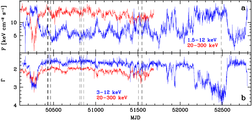
Figure 2: (a) The ASM (blue, till 2003 June 5) and BATSE (red) lightcurves with the dashed lines showing the times of the occurence of the flares. The line width is proportional to the number of flares within a given day. (b) The corresponding average spectral indices. Note the recent state transitions in 2001 September, 2002 October and 2003 May/June.

3 Flares in the soft state

The lightcurve of the flare 13 is shown in Figs. 1c and 3. Fig. 3 gives detailed PCA profiles of both the main flare and the precursor, as well as the HEXTE lightcurve, very similar in shape to the PCA one. The peak of the count rate profile of the main flare is not well fitted by an exponential function, and therefore we used a stretched exponential, $C_{0}\exp[-(|\Delta t|/\tau)^{\beta}]+C_{1}$, where $\beta=0.65\pm 0.05$, $0.70\pm 0.10$ and $\tau=17\pm 5$, $21\pm 6$ ms before and after the peak, respectively. Even this function does not provide a good overall fit ($\chi^{2}/\nu=590/220$), as the main flare appears to be superposition of several subflares much faster, $\ga 2$ ms, than the overall profile. If we fit the peak profile with the sum of two exponentials and a constant on each side of the peak (Negoro et al. 1994; F99), the shorter time scale is $\tau\simeq 7$ ms for both rise and decline, which is comparable to those obtained by F99 for the average soft-state shot (with the relative amplitude $\la 2$). The residuals for this model are very similar to those shown in Fig. 3a. After the initial fast decline, we see a slow return to the average level (see Fig. 1c) with the e-folding time of $3.2\pm 0.6$ s. On the other hand, the precursor profile (Fig. 3b) shows the rise and decline with the e-folding time as short as 1 ms and 2 ms, respectively.

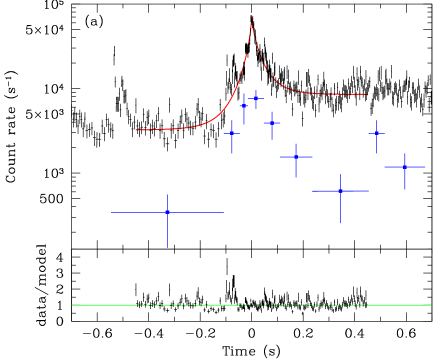
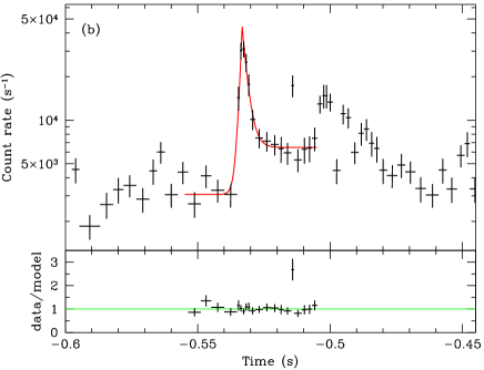
Figure 3: (a) The 2–60 keV PCA and 15–60 keV HEXTE (error bars with filled squares, multiplied by a factor of 20) lightcurves, and PCA residuals of the flare 13 fitted (solid curve) by stretched exponential rise/decline. The average PCA count rate immediately preceding the flare was $\sim 3000$ s^-1, which first increased to $\sim 4\times 10^{4}$ s^-1 over $\sim 2$ ms during the precursor, and then to the peak of $\sim 7\times 10^{4}$ s^-1 with the FWHM $\simeq 25$ ms. The flare was then followed by a period of enhanced flux for about 10 s. (b) A detailed view of the profile of the precursor, fitted (the solid curve) by exponential rise/decline.

The 3–30 keV flux during 2 ms containing the peak of the flare reached $(3.0\pm 0.6)\times 10^{-7}$ erg cm^-2 s^-1, which is $\sim 30$ times the corresponding average flux in a 16 s period before the flare [and corresponds to $L\simeq(1.4\pm 0.3)\times 10^{38}$ erg s^-1 at $d=2$ kpc, which distance we assume hereafter]. Fig. 4 shows the 3–30 keV energy flux profile as well as the average spectral indices in the spectral bands of 2–14.8 keV and 5.7–60 keV. We see a strong hardening in both bands during both the main flare and the precursor, with $\Gamma_{2-14.8}$ decreasing from $\sim 4$ to $2.2\pm 0.1$ during 10 ms around the peak of the flux, and then correlated with the flux during the $\sim 10$ s-long decline. The evolution of $\Gamma_{5.7-60}$ is from $\sim 3$ to $1.7\pm 0.2$ at the peak 10 ms. We note that an even stronger hardening occured during the precursor. All these changes are much stronger than a moderate hardening found by F99 for the soft-state shots (with the amplitude $\la 2$).

Figure 4: Evolution of the 3–30 keV flux and the average spectral indices in two bands for the flare 13.

Given the values of the flux and spectral indices at the peak, we can plot schematically the peak 3–30 keV spectrum in Fig. 5a. We also show the PCA spectrum from a 70 ms period containing the flare, which we plot normalized to the peak flux. Fig. 5a also shows the PCA spectrum from a 16 s interval preceding the flare as well as the average PCA/HEXTE spectrum from the entire observation of 2002 July 30–31. For comparison, we also show the broad-band spectrum of the soft state in 1996 June from BeppoSAX and CGRO (McConnell et al. 2002).

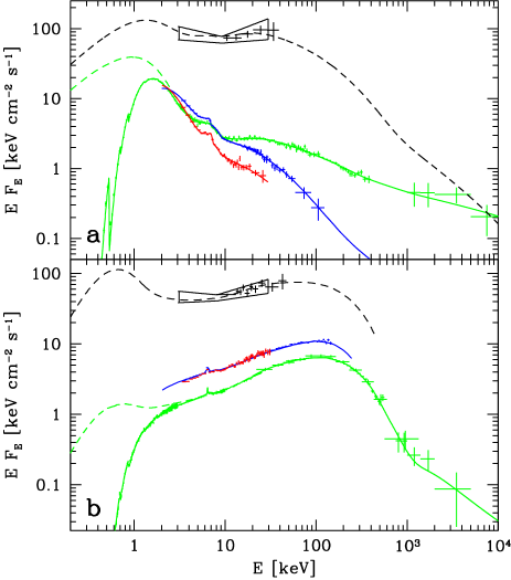
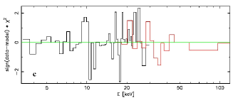
Figure 5: Spectra related to the flare (a) on 2002-07-31, with the 1996 soft state spectrum from BeppoSAX and CGRO shown for comparison in green; and (b) on 1996-12-16, with the average hard-state spectrum from CGRO and a BeppoSAX spectrum matching the CGRO data at $\la 20$ keV shown in green. On both panels, the green dashed curve shows the corresponding intrinsic spectrum before absorption. The PCA/HEXTE average spectra during the observations containing the flares, and the PCA spectra from 16 s before the flare are shown in blue and red, respectively. The black error contours show the spectra at the peak of the flare estimated from the ratios of count rates in three energy bands, and the black crosses give the PCA spectra from $\sim 0.1$–0.2 s around the peak of the flare and renormalized to the peak flux. The black dashed curves show possible blackbody/Compton scattering models. (c) Residuals to the hybrid-Compton model for the 2002 July 30–31 observation.

The last three soft-state spectra have been fitted with a hybrid Comptonization model, in which disc blackbody emission is upscattered by electrons with a Maxwellian distribution and a non-thermal tail (Coppi 1999; Gierliński et al. 1999). The tail is formed due to electron acceleration at a power-law rate with an acceleration index, $\Gamma_{\rm acc}$. Then, the steady-state electron distribution is solved for self-consistently, taking into account all important processes. The 2002 soft-state spectra are adequately described by this model. In particular, $\chi^{2}/\nu=75/81$ (assuming a 1 per cent systematic error for the PCA) for the fit to the PCA/HEXTE spectrum from the entire 2002 July 31 observation, with low $\chi^{2}$ residuals shown in Fig. 5c. We have found that the 2002 spectra have much softer tails, corresponding to $\Gamma_{\rm acc}\simeq 3.9\pm 0.6$, compared to $\Gamma_{\rm acc}\sim 2.5$ in 1996 June (Gierliński et al. 1999; Frontera et al. 2001; McConnell et al. 2002). Also, the luminosity in the tail is significantly lower than that during the 1996 soft state. In both cases, that power is much less than that in the blackbody disc emission, shown for the 1996 spectrum (which was measured at soft X-rays) by the green dashed curve in Fig. 5a.

The question arises what is the nature of the spectrum during the flare. We note that transient black-hole binaries go through the so-called very high state at high luminosities (e.g. Miyamoto et al. 1991), with a high amplitude of the high-energy tail with respect to the blackbody. Recently, Gierliński & Done (2003) have shown that the very high state spectrum of the transient XTE J1550–564 is well fitted by the hybrid model with the ratio between the power in the Comptonizing plasma to that in the blackbody disc of $\sim 1$. Then, the tail starts near the peak of the blackbody spectrum. Motivated by this, we have looked into the possibility that the flare spectrum is of similar nature, and found this indeed plausible. The black dashed curve in Fig. 5a shows the intrinsic spectrum of a possible model, with the blackbody component higher by a factor of $\sim 2$ than that during the 1996 soft state. The presence of non-thermal electrons is not constrained by the data, and we assumed that the power supplied to electron acceleration is the same as that in electron heating (similarly to the case of XTE J1550–564, Gierliński & Done 2003). The hardening at $\sim 10$ keV is due to the onset of Compton reflection (Magdziarz & Zdziarski 1995), assumed here to correspond to a solid angle of $2\pi$.

The bolometric flux of this model is $9\times 10^{-7}$ erg cm^-2 s^-1, which is $\sim 6$ times the bolometric flux of the intrinsic emission observed by BeppoSAX and CGRO in 1996, and corresponds to $L\simeq 4.5\times 10^{38}$ erg s^-1, i.e. $\sim 0.3$ of the Eddington luminosity of a $10{\rm M}_{\sun}$ star. The physical origin of the flare may be related to a disc instability close to its inner edge, in which there is a sudden conversion of energy accumulated in the Keplerian disc into magnetic heating of a hot plasma (e.g., Machida & Matsumoto 2003), or to flipping among multiple state of the accretion flow with large amplitude on short dynamical timesclaes as exhibited in recent MHD simulations by Proga & Begelman (2003). Another possibility is accumulation of a very large amount of energy in a flare above the disc surface and its subsequent fast release (e.g., Beloborodov 1999).

Interestingly, we also found two weaker flares (with the excess flux divided by rms of $\sim 8$, thus not listed in Table 1) in the 2002 soft state, during which the X-ray spectrum softened. This is opposite to the case above, indicating more than one physical scenario leading to flaring in the soft state.

4 Flares in the hard state

Figs. 1a and 6 show the count rate history of the first flare on 1996 Dec. 16. By fitting by a streched exponential, we obtain $\tau=27\pm 10$, $79\pm 24$ ms and $\beta=0.50\pm 0.08$, $0.45\pm 0.10$ during the rise and decline, respectively. Although relatively strong, this flare is representative for other hard-state flares, see, e.g. the profile of flare 9 in Fig. 1b. Note also the appearance of four flares within 16 hr on 1996 Dec. 16, and two flares within 5 hr on 1997 Jan. 17. This indicates flare clustering with the correlation time of several hours.

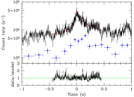
Figure 6: The 2–60 keV PCA and 15–60 keV HEXTE (error bars with filled squares, multiplied by a factor of 7) lightcurves, and PCA residuals of the flare 1 fitted (solid curve) by stretched exponential rise/decline.

Fig. 7 shows the corresponding profile in energy flux units as well as the average spectral indices in the spectral bands of 2–13 keV and 5.1–60 keV. The 3–30 keV flux during 2 ms containing the peak reached $(1.9\pm 0.3)\times 10^{-7}$ erg cm^-2 s^-1, which is $11\pm 2$ times the corresponding average flux in a 16 s period before the flare, and corresponds to $L\simeq(9\pm 1)\times 10^{37}$ erg s^-1. We now see a softening during the flare (more pronounced in the 2–13 keV band), with $\Gamma_{2-13}$ and $\Gamma_{5.1-60}$ increasing from $\sim 1.7$ to $2.0\pm 0.1$ and from $\sim 1.5$ to $1.7\pm 0.1$, respectively, averaged over 33 ms containing the peak. A similar softening during the shots in the hard state has been found by Negoro et al. (1994) and F99. Note that the X-ray spectrum at the peak is rather similar to the corresponding one of the soft-state flare.

Figure 7: Evolution of the 3–30 keV flux and the average spectral indices in two spectral bands for the hard-state flare of 1996-12-16 (No. 1 in Table 1).

Given the values of the flux and spectral indices at the peak, we can plot schematically the peak 3–30 keV spectrum in Fig. 5b, together with the PCA spectrum from a 16 s interval preceding the flare as well as the average PCA/HEXTE spectrum from the entire observation of 1996 Dec. 16. We also obtained the PCA spectrum from 0.2 s containing the flare peak, which is shown in Fig. 5b, and is fully compatible with the estimate from broad-band fluxes. For comparison, we also show the average hard-state spectrum from CGRO and BeppoSAX (McConnell et al. 2002). Given the form of the flare spectra, a large increase of the flux of seed photons for Comptonization is required, as illustrated by the black dashed curve in Fig. 5b. This model is based on those for the hard state by Frontera et al. (2001) and Di Salvo et al. (2001), where there are two thermal Comptonization regions, dominating in soft and hard X-rays, respectively. The bolometric flux of this model is $\sim 8\times 10^{-7}$ erg cm^-2 s^-1, which is $\sim 20$ times the average bolometric flux in the hard state (Z02), and corresponds to $L\simeq 3.7\times 10^{38}$ erg s^-1. Note that the similarity of the peak spectrum of this flare to that in the soft state implies that a hybrid model similar to that shown in Fig. 5a is also possible. Notably, the $\ga 10^{3}$-s flares found by Goleneetski et al. (2003) also show similar peak spectra and fluxes.

5 Statistics of the flares

An important question is that of the relation of our flares to the much weaker peaks seen in X-ray lightcurves of Cyg X-1. Apart from the issue of the applicability of the shot-noise model to Cyg X-1, we can still consider the distribution of the relative amplitudes of those peaks, or shots, with respect to the local average. That was studied by Negoro et al. (1995) and Negoro & Mineshige (2002) for the hard state. The overall shape and time scales of their shots, although with much lower amplitudes, is relatively similar to that of the 12 flares found here. Those authors have found good fits to the distribution of the peak shot count rates in 31.25 ms time bins by either an exponential or a log-normal function (with a power law strongly ruled out). Their results for $1.5\la r\la 3.5$, where $r$ is the ratio of the shot peak count rate to the average, can be expressed as the integral distribution of ${\rm d}N/{\rm d}t(>r)\sim 40\exp(-2.8r)$ s^-1 or $\sim 4\int_{r}^{\infty}{\rm d}r^{\prime}\exp(-4\ln^{2}r^{\prime})$ s^-1 (using the net exposure of 8320 s, H. Negoro, private communication).

For our hard-state flares, we have found the increase of the count rate in 32 ms bins (which is significantly lower than the actual increase seen with ms resolution) with respect to the preceding 10 s is by a factor of 6.5 for the flares 1, 3 and 9 (and slightly less for the others). Then, the rate of events stronger or equal than that is $4\times 10^{-7}$ s^-1, $1.7\times 10^{-6}$ s^-1 for the two above distributions, respectively. Given our hard-state exposure of 1.9 Ms, the former and the latter distribution predicts 0.7, 3.3 events, respectively. Thus, the flares in the hard state can represent the extreme end of the shot distribution, with its log-normal form (proposed by Negoro & Mineshige 2002) preferrred by our data.

Although shots in the soft state have been studied by F99, no distribution of their amplitudes is available. If we still apply the formula for the log-normal distribution in the hard state to the obtained relative increase of the 32-ms count rate of 9.2 for the flare 13, we obtain one predicted event per $1.3\times 10^{8}$ s, i.e., a much longer time interval than our soft-state exposure. Thus, the distribution of flare amplitudes in the soft state has most likely a different form.

References

- [1] Baganoff F. K. et al., 2001, Nat, 413, 45
- [2] Beloborodov A. M., 1999, in Poutanen J. & Svensson R., eds., High Energy Processes in Accreting Black Holes. ASP Conf. Ser. Vol. 161, San Francisco, ASP, p. 295
- [3] Boller T., Brandt W.N., Fabian A.C., Fink H.H., 1997, MNRAS, 289, 393
- [4] Boldt, E., 1977, Ann. N. Y. Ac. Sci., 302, 329
- [5] Bowyer S., Byram E.T., Chubb T.A., Friedman M., 1965, Sci, 147, 394
- [6] Brandt W. N., Boller T., Fabian A. C., Ruszkowski M., 1999, MNRAS, 303, L53
- [7] Chaput, C. et al., 2000, ApJ, 541, 1026
- [8] Churazov E., Gilfanov M., Revnivtsev M., 2001, MNRAS, 321, 759
- [9] Coppi P. S., 1999, in Poutanen J. & Svensson R., eds., High Energy Processes in Accreting Black Holes, ASP Conf. Ser. Vol. 161, San Francisco, ASP, p. 375
- [10] Di Salvo T., Done C., Życki P. T., Burderi L., Robba N. R., 2001, ApJ, 547, 1024
- [11] Feng Y. X., Li T. P., Chen L., 1999, ApJ, 514, 373 (F99)
- [12] Frontera F. et al., 2001, ApJ, 546, 1027
- [13] Gierliński M., Done C., 2003, MNRAS, in press
- [14] Gierliński M., Zdziarski A. A., Done C., Johnson W. N., Ebisawa K., Ueda Y., Haardt F., Phlips B. F., 1997, MNRAS, 288, 958
- [15] Gierliński M., Zdziarski A. A., Poutanen J., Coppi P. S., Ebisawa K., Johnson W. N., 1999, MNRAS, 309, 496
- [16] Golenetskii S., Aptekar R., Frederiks D., Mazets E., Palshin V., Hurley K., Cline T., Stern B., 2003, ApJ, submitted
- [17] Lin D., Smith I.A., Böttcher M., Liang E.P., 2000, ApJ, 531, 963
- [Lochner 1991] Lochner J.C., Swank J.H., Szymkowiak A.E., 1991, ApJ, 376, 295
- [Machida 2003] Machida M., Matsumoto R., 2003, ApJ, 585, 429
- [18] Magdziarz P., Zdziarski A. A., 1995, MNRAS, 273, 837
- [19] McConnell M. L. et al., 2002, ApJ, 572, 984
- [20] Meekins J. F., Wood K. S., Hedler R. L., Byram E. T., Yentis D. J., Chubb T. A., Friedman H., 1984, ApJ, 278, 288
- [Miyamoto 1991] Miyamoto S., Kimura K., Kitamoto S., Dotani T., Ebisawa K., 1991, ApJ, 383, 784
- [21] Negoro H., Mineshige S., 2002, PASJ, 54, L69
- [22] Negoro H., Miyamoto S., Kitamoto S., 1994, ApJ, 423, L127
- [23] Negoro H., Kitamoto S., Takeuchi M., Mineshige S., 1995, ApJ, 452, L49
- [Pottschmidt 1998] Pottschmidt K., Koenig M., Wilms J., Staubert R., 1998, A&A, 334, 201
- [24] Pounds K. A., Done C., Osborne J. P., 1995, MNRAS, 277, L5
- [25] Press W. H., Schechter P., 1974, ApJ, 193, 437
- [26] Proga D., Begelman M. C., 2003, ApJ, in press
- [27] Revnivtsev M., Gilfanov M., Churazov E., 2000, A&A, 363, 1013
- [28] Rothschild R. E., Boldt E. A., Holt S. S., Serlemitsos P. J., 1974, ApJ, 189, L13
- [29] Rothschild R. E., Boldt E. A., Holt S. S., Serlemitsos P. J., 1977, ApJ, 213, 818
- [30] Stern B.E., Beloborodov A.M., Poutanen J., 2001, ApJ, 555, 829
- [31] Sunyaev R., Revnivtsev M., 2000, A&A, 358, 617
- [Uttley 2001] Uttley P., McHardy I.M., 2001, MNRAS, 323, L26
- [32] Weisskopf M.C., Sutherland P.G., 1978, ApJ, 221, 228
- [33] Zdziarski A. A., Poutanen J., Paciesas W.S., Wen L., 2002, ApJ, 578, 357 (Z02)