Optimal Techniques in Two-dimensional Spectroscopy: Background Subtraction for the 21st Century

Abstract

In two-dimensional spectrographs, the optical distortions in the spatial and dispersion directions produce variations in the sub-pixel sampling of the background spectrum. Using knowledge of the camera distortions and the curvature of the spectral features, one can recover information regarding the background spectrum on wavelength scales much smaller than a pixel. As a result, one can propagate this better-sampled background spectrum through inverses of the distortion and rectification transformations, and accurately model the background spectrum in two-dimensional spectra for which the distortions have not been removed (i.e. the data have not been rebinned/rectified). The procedure, as outlined in this paper, is extremely insensitive to cosmic rays, hot pixels, etc. Because of this insensitivity to discrepant pixels, sky modeling and subtraction need not be performed as one of the later steps in a reduction pipeline. Sky-subtraction can now be performed as one of the earliest tasks, perhaps just after dividing by a flat-field. Because subtraction of the background can be performed without having to “clean” cosmic rays, such bad pixel values can be trivially identified after removal of the two-dimensional sky background.

1 Introduction

For more than 100 years, optical astronomers have employed long-slit spectrographs to study the internal physics of heavenly objects. Such data contain the target’s spectrum dispersed at every location along a single position angle on the sky (unless the target is an unresolved source). Unfortunately, at every location along the slit, one also collects photons from the night-sky emission. This background must be removed from the data in order to reveal the spectrum of the intended target. With the expansion of spectroscopy to wide fields-of-view, one can employ multi-slit aperture plates to collect spectra for many objects simultaneously, or observe with a very long slit. Over the past several years, important advances have been made in the art of background subtraction, though largely in the area of small-aperture spectroscopy, either with fibers or “micro-slits” (e.g., Kurtz & Mink, 2000; Glazebrook & Bland-Hawthorn, 2001; Viton & Milliard, 2003). However, or typical long- and multi-slit spectroscopy, the most common reduction procedures do not make optimal use of the data, and the resultant spectra with which one must perform one’s science suffer in quality compared to what is achievable with more modern techniques and modest computing power.

This paper outlines a new technique which makes optimal use of the data to accurately perform the subtraction of the unwanted background spectrum from two-dimensional spectra before any rebinning of the data is performed. In the procedure one makes full use of the spectrograph distortions to improve the sampling of the sky background spectrum. The quality of the background subtraction is completely insensitive to the magnitude of the distortions imposed by the spectrograph’s camera, to the severity of the curvature of the spectral lines that is caused by the dispersive element, or even to any tilting of individual slitlets in an aperture mask. Furthermore, by explicitly employing maps of the y-distortion and line curvature in a two-dimensional spectrum, the model two-dimensional background spectrum not only follows the same line curvature and y-distortion as the data, but the spectral features are sampled (pixelated) in exactly the same way as the features are sampled in the raw observations. As a result, when one subtracts the model from the data, there are absolutely no sharp residuals at the edges of night-sky emission lines. With more traditional methods, two-dimensional spectra must be rectified before one can perform the subtraction of the background; such rectification procedures introduce artifacts into the data, particularly when the sampling is poor. These artifacts can manifest themselves as sharp residuals at the edges of features with strong gradients, e.g., the night sky lines. Furthermore, in traditional methods, observers are required to identify (and remove) cosmic rays and other bad pixels before rebinning the data. With the method discussed in this paper, the sky subtraction is performed before the data have been rebinned, and, as a result, cosmic rays can be “cleaned” after the task of removing the sky background.

In the following sections, the method for fitting the two-dimensional night-sky background is described. Subsequently, this powerful new technique is applied to data riddled with cosmic rays and bright night-sky emission lines. The examples include data from three spectrographs, in which the data span a range of sampling from marginal (LRIS), to slightly under-sampled (NIRSPEC), to grossly under-sampled (MIKE). And finally the the advantages of this method over traditional methods will be summarized.

2 The Basic Procedure

Two-dimensional spectra, when ultimately imaged onto a detector, suffer from two problems that must be dealt with before or during the process of background subtraction: (1) the fact that the two-dimensional spectra are not aligned exactly along the rows (or columns) of the detector and are often curved with respect to the natural coordinate system of the detector (the y-distortion); and (2) the general tendency for dispersers to impose a wavelength-dependent line curvature onto the two-dimensional spectra (which may have already been tilted or curved if the slit has been so cut into the aperture plate). Furthermore, the coarse pixel sizes of modern detectors impose a third problem which normally limits the accuracy with which one could previously deal with the first two.

In order to discuss these issues and their resolution, we first define the image of two-dimensional spectroscopic data as $P(x,y)$, where $(x,y)$ are pixel coordinates in the system of the original image (e.g., a CCD frame). Because of distortions imposed by the optics, the spatial coordinate on the sky, $y_{t}$, for a given pixel $(x,y)$ is a non-linear function, $y_{t}=Y(x,y)$. Furthermore, the wavelength of light, $\lambda$, incident onto a pixel $(x,y)$ is also a non-linear function of image position. For the purposes of modeling the two-dimensional background spectrum, we are less concerned with the actual wavelength, $\lambda$, of incident light than we are with the fact that there exists a coordinate system, $(x_{r},y_{t})$, in which $x_{r}$ is a wavelength-dependent coordinate that is orthogonal to the spatial coordinate $y_{t}$. The transformation to this system is $x_{r}=X(x,y_{t})$ such that the wavelength of light incident on a pixel can be written $\lambda=L(x_{r})$, where $x_{r}=X(x,Y(x,y))$. Thus there exists a convenient coordinate system $(x_{r},y_{t})$ for which $\partial L/\partial y_{t}=0$. The transformations $Y(x,y)$ and $X(x,y_{t})$ can be measured with great precision from comparison lamp spectra or from the night-sky features themselves (see, e.g., Kelson et al., 2000, for a description of a robust algorithm using FFTs and cross-correlations in order to make full use of the available data to map these distortions).

With knowledge of $Y(x,y)$ and $X(x,y_{t})$, the traditional method of sky-subtraction required one to interpolate $P(x,y)$ onto a regular grid in $(x_{r},y_{t})$ before fitting the two-dimensional sky spectrum at every individual interval of $\lambda$ in the rebinned image. Unfortunately, the process of rebinning the data (1) introduces correlated noise; (2) smears cosmic rays and other bad pixels which might not have been flagged/cleaned beforehand; and (3) produces artifacts at the edges of sharp features. This last problem sometimes leads users to invoke high spatial orders in the fitting of the sky background in order to subtract such artifacts at the edges of sky lines. Furthermore, the rebinning of the data forces every sky spectrum used in the fit to have a common pixelation. This process limits one’s ability to accurately model the two-dimensional sky spectrum where gradients (e.g., $\partial P/\partial x_{r}$) can be large.

Instead of rebinning the data before performing the modeling of the two-dimensional sky spectrum, we propose that one should perform a least-squares fit to the sky spectrum using the original data-frame, in which the distortions and line curvature have not been removed. Using $y_{t}=Y(x,y)$ and $x_{r}=X(x,y_{t})$ one should model the background spectrum in $P(x,y)$ as a function of the rectified coordinates $(x_{r},y_{t})$.

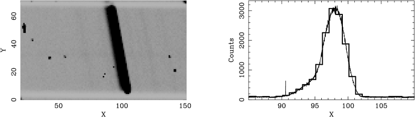
Figure 1: (left) A subsection of an LRIS two-dimensional spectrum surrounding the 5577Å night-sky emission line. (right) The thick line shows the intensity of the 5577Å line from a single CCD row. The thin line shows the value of every pixel in the left-hand panel, plotted as a function of its rectified position, $x_{r}=X(x,y_{t})$, along the wavelength-dependent coordinate in the rectified coordinate system. Note that the shape of the line is actually quite well sampled as a result of the tilt of the spectral line, due to both the tilting of the slit on the aperture plate and the line curvature imposed by the instrument’s grating. If the data were to be rebinned, this over-sampling would be lost. Note the spike at $x\approx 91$, at which a cosmic ray is clearly visible above the rest of the data (see Figure 2).

Each pixel in the original image represents an integral of the flux within a box the size of 1 pixel, but in the analysis each observed pixel’s location is assumed to be $(x_{r},y_{t})$, rather than $(x,y)$. In this way, each pixel samples the sky spectrum at a known sub-pixel position. Figure 1, in which a small section of an LRIS (Oke et al., 1995) spectrum is shown, demonstrates the utility of this change in coordinate systems. The left-hand panel shows a region around 5577Å in a short two-dimensional spectrum obtained using the 600 g/mm grating ($\sim 1.28$Å/pixel). The resolution is $\sim 3.5$ pixels (FWHM). Note in the image how pixelated the edges of the sky line are. Rebinning such data would lead to spatially periodic artifacts along the edge of the line. In the right-hand panel, the thick line shows the spectrum from one row, indicating how pixelated and poorly sampled the gradients in the line profile are in a given CCD row. The thin line shows the pixel values in the image $P(x,y)$ as a function of $x_{r}=X(x,y_{t})$, revealing how well the CCD frame samples the sky spectrum. Such over-sampling is lost when one rebins the data.

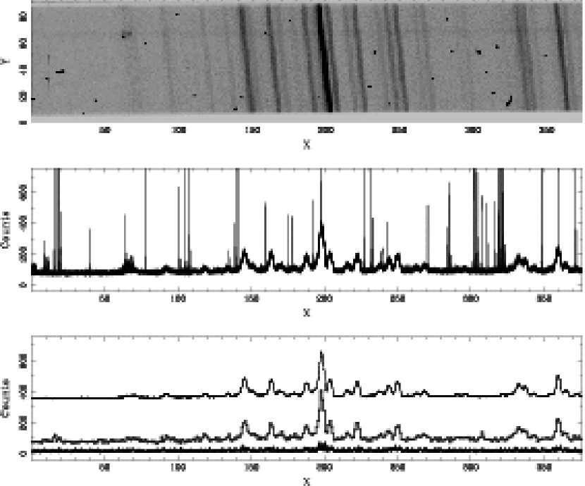
Figure 2: (top) A subsection of an LRIS two-dimensional spectrum surrounding the 6300Å night-sky emission line. (middle) The raw spectrum as sampled in every row of the image section, where the pixel values are plotted as a function of $x_{r}$ (the rectified wavelength-dependent coordinate). Note that, as in Figure 1 the night-sky emission lines are well-sampled as a result of the distortions and line curvature. Also note that many spikes in the data, representing cosmic rays and other bad pixels, are clearly visible. (bottom) The thick line shows the spectrum from a single row, indicating the coarse sampling by the LRIS pixels. Artificially shifted higher is the 30%-smoothed version of the spectrum shown in the middle figure. The line hovering near zero in the bottom panel shows the $4\times\sigma$ scatter as a function of $x_{r}$. Using the percentile-smoothing of the data along the $x_{r}$ direction together with a robust $\sigma$-clipping algorithm allows one to reject cosmic rays and bad pixels from the fitting of the B-spline.

In Figure 2, a larger section of the same LRIS frame is shown in the top panel. The middle panel shows $P(x,y)$ plotted as a function of $X(x,y_{t})$. Note that many spikes in the data are visible. These discrepant points correspond to cosmic rays and other bad pixels. Fortunately, the sky spectrum is actually quite over-sampled in the rectified coordinate system, with many redundant measurements of the sky at nearly the same sub-pixel location.

Because of the redundancy in the sampling of the background spectrum, it becomes straightforward to identify the cosmic rays and bad pixels, even when they appear where gradients in the background spectrum are large. In the bottom panel, the thick line shows the spectrum sampled by a single row. The smooth line, shifted towards positive values, is a smoothed version of the data in the middle panel. The smoothing that was adopted was a running 30th-percentile within a window 30 data elements wide in $x_{r}$. In the bottom panel, we also show the running $4\sigma$ scatter (robustly determined) within the same sliding window. By comparing $P(x,y)$ with the smoothed spectrum in the middle panel, one can employ a simple $\sigma$-clipping algorithm to reject the cosmic rays and bad pixels, even where there are strong gradients in $P(x,y)$. Normally, the rejection/identification of cosmic rays or bad pixels involves the comparison of a pixel in an image with its nearest neighbors. However, because of the poor sampling of strong gradients in the background spectrum, one should compare a given pixel to those nearest only in $x_{r}=X(x,Y(x,y))$, i.e. sampled at the same sub-pixel interval. Thus, the smoothing is done on a copy of the array $P(x,y)$ that has been sorted in order of increasing $x_{r}$. Because the line curvature (plus the additional tilt of the slitlet) has improved the sampling of the night-sky spectrum, cosmic rays that fall where there are strong gradients in the sky spectrum can still be robustly identified, as other CCD rows have sampled the sky spectrum with similar sub-pixel sampling as at the location of a given cosmic ray.

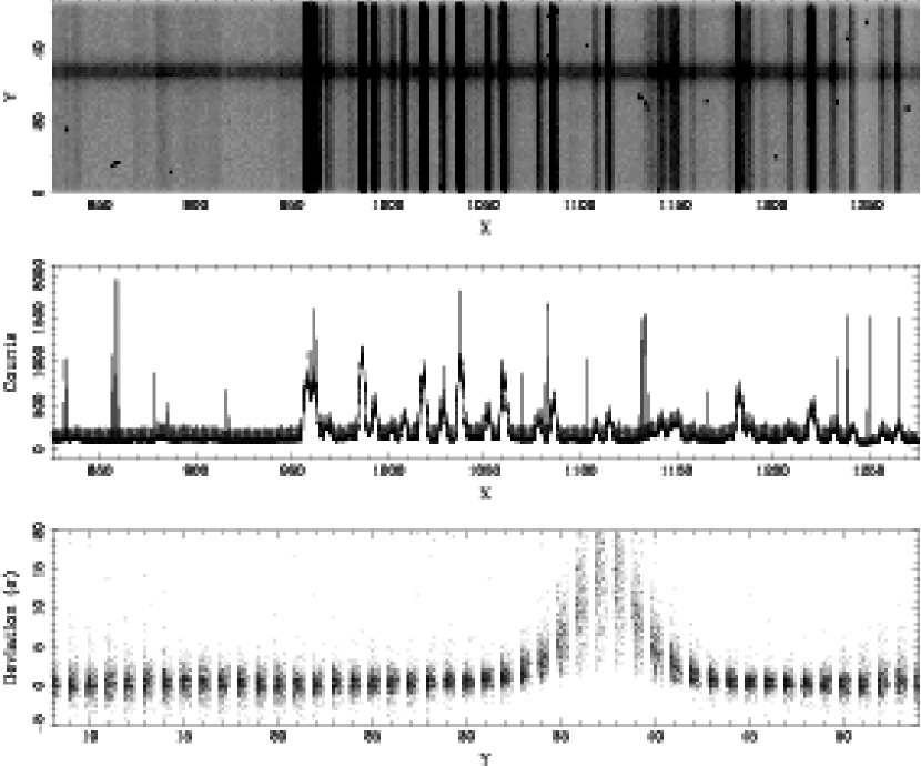
Figure 3: (top) A subsection of an LRIS two-dimensional spectrum in the red, with a bright object in the slit. (middle) The spectrum as sampled in every row of the image section shown, where the pixel values are plotted as a function of $x_{r}$ (the wavelength-dependent coordinate in the rectified coordinate system). Note that while many cosmic rays are clearly visible, there also appear to be spikes peaking above the data at regular intervals in $x_{r}$. These discrepant pixels have counts which are dominated by flux from the object. (bottom) The deviations from the percentile-smoothed data plotted as a function of spatial position along the slit. Note that the same $\sigma$-clipping algorithm that rejects cosmic rays also rejects pixels contaminated by objects.

While cosmic rays and other bad pixel values tend to be isolated sharp features, objects are generally extended in $(x_{r},y_{t})$. The top panel of Figure 3 shows a subsection of data for a slitlet containing a bright object. The middle panel shows every pixel $P(x,y)$ plotted, again, as a function of $X(x,y_{t})$. Most of the pixels in the data only contain flux from the night-sky background, and these data points follow a locus in the figure with very small scatter. As in Figure 2, the cosmic rays are clearly visible above the well-defined background spectrum. Also visible, however, is a collection of points in the data which peak above the sky spectrum at regular intervals of $X(x,y_{t})$. If we take the residuals of $P(x,y)$ from the robustly-smoothed version of the sky spectrum in the middle panel, and plot the statistical significance of those residuals against the spatial coordinate $y_{t}=Y(x,y)$, as in the bottom panel of the figure, the object pixels are clearly visible as a significant positive deviation from zero. By employing the $\sigma$-clipping described above for flagging cosmic rays, one also singles out those pixels that are significantly contaminated by flux from the object. In general a choice of clipping at 3 or $4\sigma$ is very effective at rejecting cosmic rays from the fit to the sky background, and it also rejects objects which could seriously affect the fit to the sky. Faint objects, which do not peak above the adopted threshold tend not to affect the modeling of the sky and most such objects tend to cover too small a spatial area to adversely affect the fit anyway. While a clipping method works sufficiently well for most applications, one can straightforwardly implement an input set of sky apertures, outside of which pixels are simply ignored. Sky apertures may be specifically useful in very short slitlets, where the the sky covers $\lower 1.29167pt\hbox{$\scriptscriptstyle\;\buildrel<\over{\sim}\;$}10\%$ of the spatial extent of the slit.

Once the discrepant pixels are rejected, a bivariate B-spline (e.g., de Boor, 1978; Dierckx, 1993) is constructed as an approximation to the remaining remaining data points as a function of their positions. However, the pixel values are not considered to represent a bivariate function of $(x,y)$ (the original CCD coordinates) but the data are treated as a bivariate function of $(x_{r},y_{t})=(X(x,Y(x,y)),Y(x,y))$. In the author’s implementation of the method, the DIERCKX surface- and curve-fitting library available from NETLIB was used. This library allows one to weight each pixel during the fit for the B-spline coefficients, and these weights were set equal to the inverse of the expected noise.

When fitting for the B-spline representation of a bivariate dataset, the smoothness of the model is set by the density of knots in the two cardinal directions. In the simplest construction of the two-dimensional sky background, the knot locations, $t_{x}$ and $t_{y}$, are chosen with a high density in $x_{r}$ such that $t_{x}=\{{\rm min}(x_{r}),{\rm min}(x_{r})+1,\ldots,{\rm max}(x_{r})\}$ with intervals of $\Delta x_{r}=1$. The knots in $y_{t}$ are chosen to be $t_{y}=\{{\rm min}(y_{t}),{\rm max}(y_{t})\}$, where the minima and maxima in $x_{r}$ and $y_{t}$ are derived for the slit being analyzed. In this way, the B-spline is non-parametric function in $x_{r}$ and a polynomial of order $k_{y}$ in $y_{t}$. The choice of $k_{y}\in\{1,3,5,\ldots\}$ sets the order of the spatial variation in the sky spectrum at a fixed $x_{r}$ (e.g., fixed $\lambda$).

With the default choice of knots in $x_{r}$ described in the previous paragraph, the fit to the data very nearly approximates an interpolating spline along the wavelength-dependent coordinate. However, the B-spline was generated using data with finer sampling than that available in a single CCD row. As a result, the spline is a smooth representation of the sky spectrum at those locations $(x_{r},y_{t})$ in the original data frame. One can reduce the number of knots in $t_{x}$ to impose greater smoothness on the model sky spectrum in those ranges of $x_{r}$ with little structure, while leaving a higher density of knots near bright night-sky emission lines in order to better match the gradients there. While such optimization of the knots in $t_{x}$ can improve the background modeling with particularly noisy data, the selection of $t_{x}$ described above is generally sufficient. One can also insert more knots in $t_{y}$ to model more complicated spatial variation in the sky (at fixed $\lambda$). With clever placement of knots in the spatial direction, the model can better map high-frequency spatial variations such as in data containing residual fringes in the very red portions of a spectrum. If the spatial variation in the sky spectrum is expected to be negligible, such as in very short slits, a one-dimensional B-spline can be fit to the values of $P(x,y)$ as a univariate function of $x_{r}$.

Regardless of the complexity of the knot placement, the B-spline representation of the data is well-behaved because every pixel location in the original image, $(x,y)$ has a correspondingly unique, rectified coordinate $(x_{r},y_{t})$. As a result the bivariate fit is well-defined and computationally inexpensive to construct. Once the B-spline representation has been computed, it can be quickly evaluated at every $(x_{r},y_{t})$ location in the spectrum being analyzed. In this way, the two-dimensional background spectrum is only evaluated at the locations where the original pixels exist. Therefore no interpolation at sub-pixel locations (in $x,y$) occurs in the original data frame. As a result, there are no artifacts at strong gradients.

Some examples of the application of this method of optimal background subtraction are shown in the next section. The examples shown below used the simplest knot selection in the above discussion. No optimization of knot location was implemented. Finally, the examples were generated using $k_{x}=3$ and $k_{y}=1$.

3 Examples

3.1 LRIS

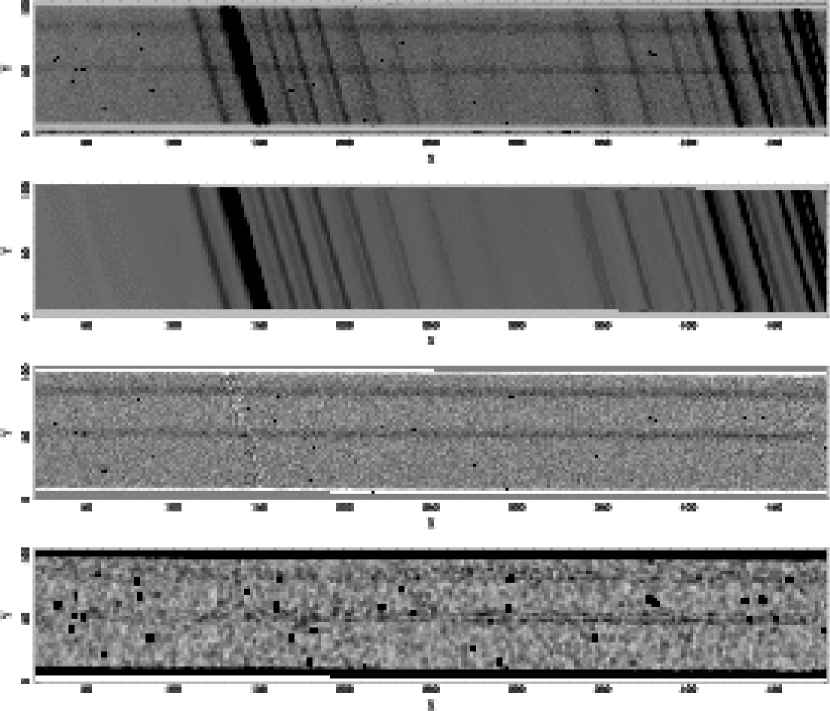
Figure 4: (top) A subsection of an LRIS two-dimensional spectrum covering from Na I to 6300Å. (top-middle) The two-dimensional fit to those pixels remaining after the $\sigma$-clipping. (bottom-middle) The background-subtracted spectrum. (bottom) An $rms$-smoothed image of the background-subtracted spectrum, divided by the expected noise (photon and read noise). Other than at the locations of the cosmic rays, the noise in the final sky-subtracted two-dimensional spectrum has no additional artifacts or unexpected features, such as would have arisen at the edges of rebinned night-sky emission lines.

The top panel of Figure 4 shows a section of two-dimensional spectrum from one strongly tilted slitlet. The wavelength range covers from blueward of Na I to approximately 6300Å. The second panel shows the model sky spectrum, derived using the new method. The third panel shows the difference between the two (i.e., the background-subtracted spectrum). Note how well the night-sky emission lines are subtracted, with no residual systematic structure. The bottom panel shows an $rms$-smoothed version of the background-subtracted image, normalized by the expected noise. This representation of the data illustrates that there is no additional noise at the locations of the sharp sky lines.

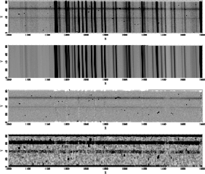
Figure 5: Same as in Figure 4 but for a different slitlet, between 7000Å and 7700Å.

Figure 5 follows a similar format as Figure 4 but for a different slitlet, and for a wavelength range 7000Å $\lower 1.29167pt\hbox{$\scriptscriptstyle\;\buildrel<\over{\sim}\;$}\lambda\lower 1.29167pt\hbox{$\scriptscriptstyle\;\buildrel<\over{\sim}\;$}$ 7700Å. As in the previous figure, the background subtraction is free of any residual systematic structure, and the noise in the background-subtracted image is as expected.

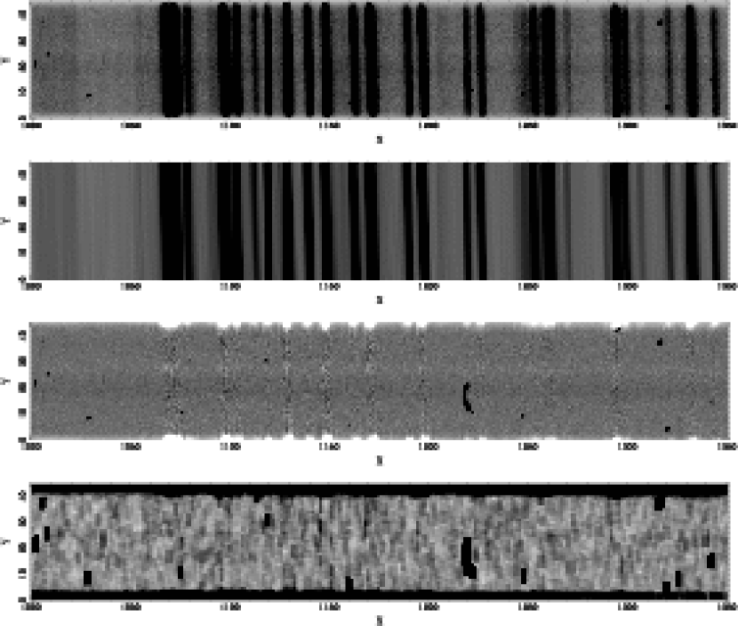
Figure 6: Same as in Figure 4 but for a short slitlet in which a serious cosmic ray sits along the top of a sky line. The robust $\sigma$-clipping algorithm easily handles such nasty occurrences.

Figure 6 shows a section of data with a wavelength range 7200Å $\lower 1.29167pt\hbox{$\scriptscriptstyle\;\buildrel<\over{\sim}\;$}\lambda\lower 1.29167pt\hbox{$\scriptscriptstyle\;\buildrel<\over{\sim}\;$}$ 7600Å. This section has a very strong cosmic ray at $(x,y)\approx(1220,15)$ that sits along a large portion of a sky line. Note how clean the sky-subtracted image is, again, with no systematic residuals at the locations of bright lines.

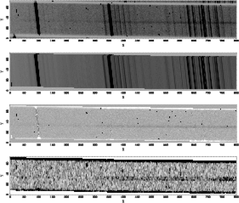
Figure 7: Same as in Figure 4 but for a tilted slit covering from 5500Å to 6500Å. Also note the strong gradient in the $y$-distortion with wavelength ($\partial Y/\partial x$). Note how cleanly 5577Å is subtracted, leaving only the expected level of Poisson noise.

Figure 7 shows a section of data with a wavelength range 5500Å $\lower 1.29167pt\hbox{$\scriptscriptstyle\;\buildrel<\over{\sim}\;$}\lambda\lower 1.29167pt\hbox{$\scriptscriptstyle\;\buildrel<\over{\sim}\;$}$ 6500Å. These data were taken from a slitlet at the edge of the LRIS field, at which the $y$-distortion, $Y(x,y)$, has a very strong derivative with respect to $x$. Note how cleanly the bright sky lines 5577Å, 5890Å, 5896Å, 6300Å, etc., are modeled and subtracted. As in the previous examples, there are no systematic residuals at the locations of bright night-sky features.

3.2 NIRSPEC

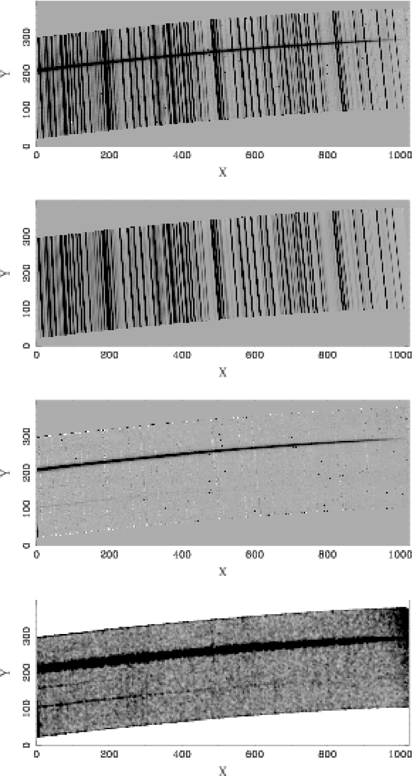
Figure 8: A single $H$-band long-slit spectrum obtained with NIRSPEC. The distortions are quite large, and the sampling is poor. Note how cleanly the night sky emission lines are subtracted, leaving only the expected level of Poisson noise.

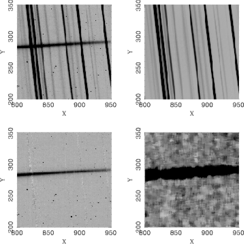
Figure 9: A section of the data in Figure 8. Note the coarse sampling (first panel). The second panel shows the model background spectrum for the same section, in which sampling in the model is identical. As discussed in the text, it is the exact reproduction of the sampling that allows one to remove the sharp features in the background with great accuracy. Extraction of the object spectrum can be performed with or without rebinning the data, depending on the needs of the individual observer.

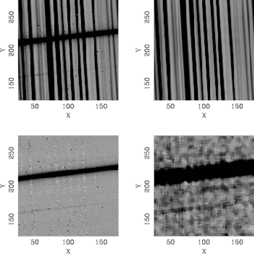
Figure 10: Same as in Figure 9, but for a different section of the NIRSPEC data.

Figure 8 shows a two-dimensional $H$-band spectrum obtained with NIRSPEC (McLean et al., 1998). The dispersion is approximately 2.8Å/pixel. The distortions in the data are large, and the sampling is poor. Small sections of these data are also shown in Figures 9 and 10. In this example, the knots in the dispersion direction were located at half-pixel intervals. This choice was motivated by the strong distortions and length of the slit. Together these allow for higher resolution in the reconstructed background spectrum.

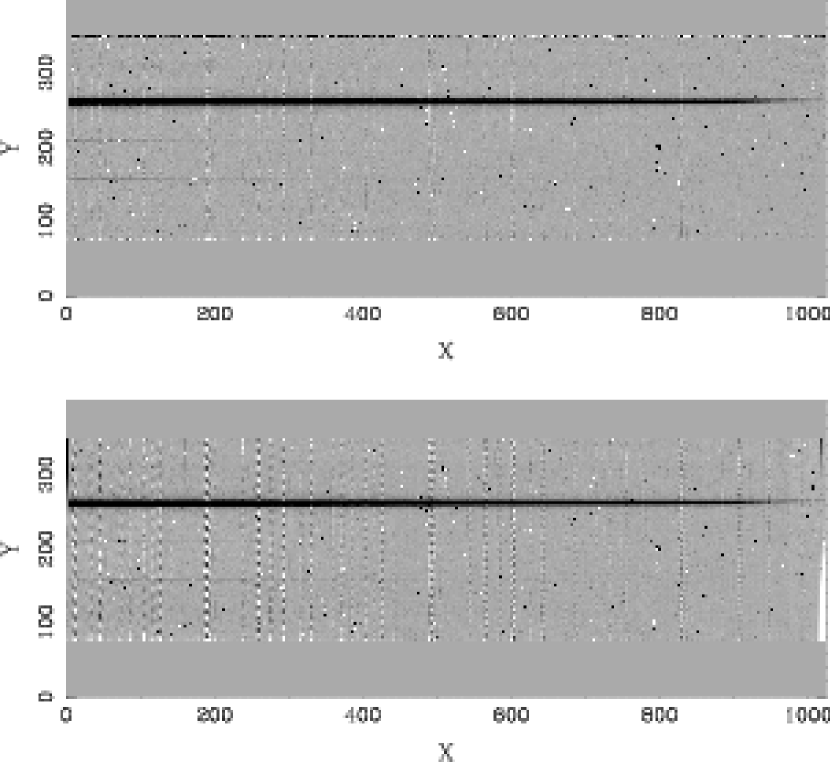
Figure 11: (top) Rectified two-dimensional sky-subtracted spectrum from Figure 8, where the rectification was performed after the task of sky-subtraction. (bottom) The same data frame but where the sky subtraction was performed after rectification of the data. By rebinning the under-sampled night sky lines, one is left with periodic artifacts in the data. In the top panel the night sky background was subtracted from the original unrebinned data prior to rectification. As a result, the noise in the sky is rebinned but not the sharp features themselves.

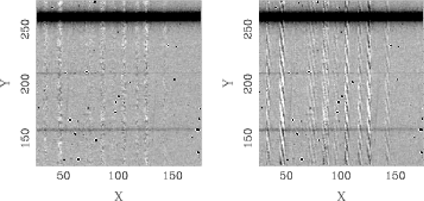
Figure 12: (left) A subsection of the rectified data, where the task of sky-subtraction was performed first; (right) a subsection of the rectified data, where the task of sky-subtraction was performed after rebinning the data. Undesired artifacts are clearly visible in the right-hand panel at the locations of the under-sampled night sky emission lines.

Even in coarsely sampled near-IR spectra, the method provides a two-dimensional model of the background with identical sampling as in the original data. Thus, the sky background subtracts cleanly, with no systematic residuals at the locations of the night sky emission lines. When the sampling is this coarse, the observer should avoid interpolating sharp features, and observers now can choose whether to rebin the sharp features in the raw data or to rebin the sky-subtracted frame. Figures 11 and 12 employ these NIRSPEC data to directly compare this new methodology for sky-subtraction with traditional procedures. In the figures, we show the NIRSPEC data in two states: (1) sky-subtracted first and rectified second; and (2) rectified first and sky-subtracted second. In the latter form, strong, periodic artifacts are plainly visible at the locations of the night sky emission lines, where the under-sampled edges were rebinned. In the former, where the task of sky-subtraction was performed first, no sharp gradients remain in the data to introduce artifacts into the rectified frame. While this example shows a comparison of rectified two-dimensional sky-subtracted data, some readers may choose not to rebin their two-dimensional spectra at all, and opt for extracting one-dimensional spectra directly from the unrectified background-subtracted frames (using knowledge of the two-dimensional wavelength solution).

3.3 MIKE

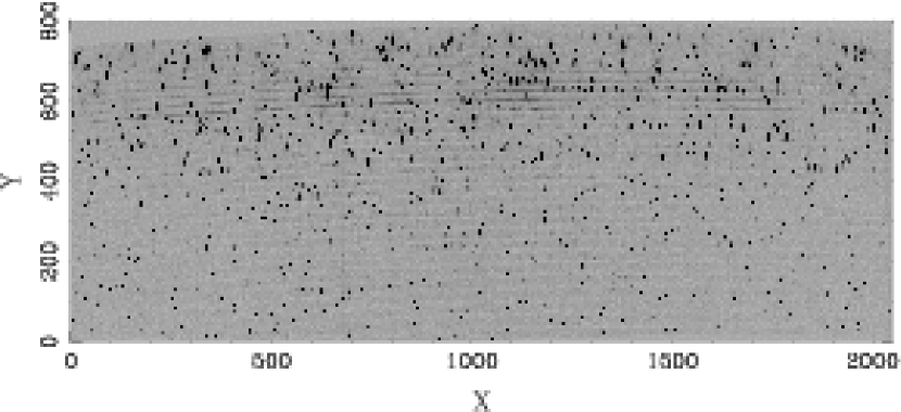
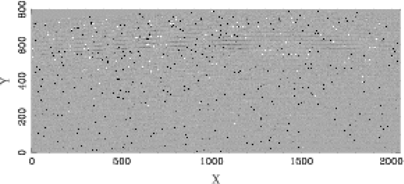
Figure 13: (a) One hour exposure of a QSO at $z=5.8$ using the red side of the MIKE echelle spectrograph on the Clay telescope at Magellan. This exposure covers order #62 (bottom, central wavelength $\sim 5540$Å) through order #33 (top, central wavelength $\sim 10300$Å). The data were binned $2\times 2$, effectively increasing the fraction of the image contaminated by cosmic rays by a factor of four. The binned data also have a dispersion of $\sim 0.1$Å/pixel. Because the data were binned, the night sky emission lines are heavily under-sampled and traditional rectification and sky subtraction techniques introduce artifacts into the data (see Figure 15). (b) Same as (a) but with the background subtracted from it.

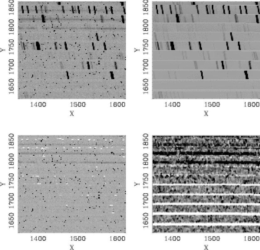
Figure 14: A subsection of the data shown in Figure 13. This section of the data has little order curvature, but the line curvature is clearly visible. With accurate maps of the distortions and line curvature, the bivariate B-spline accurately recovers the night sky spectrum at wavelength intervals smaller than a pixel, leaving only the object spectrum, cosmic-rays, and Poisson noise.

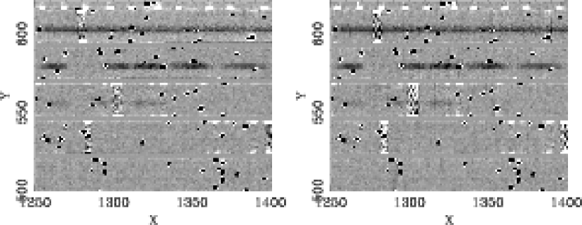
Figure 15: (left) A section of the rectified two-dimensional sky-subtracted spectrum from Figure 13, where the rectification was performed after the task of sky-subtraction. (right) The same data frame but where the rectification was performed before sky subtraction. By rebinning the under-sampled night sky lines, one is left with periodic artifacts in the data. By rectifying the sky-subtracted frame, one rebins the noise in the sky but not the sharp features themselves. Of course if one is only interested in one-dimensional spectra, then the data need not ever be rebinned.

Figures 13 – 15 show data from a one hour integration with the red side of the MIKE echelle spectrograph on the Clay 6.5m telescope at Magellan. Because the optical path in MIKE (Bernstein et al., 2003) involves using one prism as the primary disperser and the cross-disperser, the orders have large curvature and the spectra themselves show large line curvature. This exposure covers order #62 (bottom, central wavelength $\sim 5540$Å) through order #33 (top, central wavelength $\sim 10300$Å). The data had been binned $2\times 2$ while reading the CCD to avoid being read-noise dominated, even with the one hour integration. The binning increases the fraction of the image contaminated by cosmic rays by a factor of four, and reduces the spatial extent of the slit to about 20 pixels. Many users also use $1\times 3$ and even $2\times 4$ binning with MIKE, and as a result, most data obtained with MIKE will be severely under-sampled, and the binning leads to higher contamination rates with cosmic rays.

In Figure 15 we show a direct comparison of a portion of the rectified sky-subtracted MIKE data (similar to the comparison for NIRSPEC data in Figure 11). While at such high resolution the night sky lines do not affect much of the data, one may still wish to recover accurate estimates of the object flux at the locations of the sky lines. In the right-hand panel of Figure 15 there are clear artifacts at the locations of the sky-lines and such artifacts render the science data useless at those wavelengths. In the left-hand panel, the object spectrum is not contaminated by the artifacts introduced by the rebinning of night sky lines.

The examples shown in this section illustrate a range of results from the modeling procedure outlined in this paper. In all cases, when the distortions and line curvature are accurately known, the sky background shows very little spatial variation when fit in the rectified coordinate system (see §2). The need for a high spatial order is only required when using traditional methods, and artifacts at the edges of sky lines are not well modeled with low-order polynomials. Because of this, observers can also apply this method to short slitlets using one-sided sky, restricting the B-spline to one dimension (wavelength) or perhaps only limiting the spatial order to $k_{y}=1$. In such cases, the only factor limiting the accuracy of the sky subtraction would be flat-fielding and other techniques may prove more valuable (e.g., Glazebrook & Bland-Hawthorn, 2001).

4 Summary

This paper describes a new method for modeling the background in two-dimensional slit spectroscopy. This method makes full use of the data in its “raw” state — before the data have been rectified (rebinned). The distortions inherent in the data provide the means by which the background spectrum can be accurately modeled at repeated sub-pixel locations. Because of the improved sampling of the background spectrum in the original data compared to a rectified image, one can also robustly reject pixels contaminated with cosmic rays and bright objects. Because of these advantages over traditional background-subtraction techniques, the task of subtracting the two-dimensional background spectrum should now be performed as one of the first steps in any pipeline of spectroscopic reduction, even before cosmic rays and other bad pixels have been “cleaned”.

The subtraction of the background can now be performed on raw spectra, riddled with cosmic rays. As a result, the procedure can be adopted as one of the first steps in a pipeline for spectral reduction, and not as one of the last. The task is computationally inexpensive and can allow observers to quickly analyze incoming data at the telescope, assuming the distortion maps have been characterized from calibration data during the previous afternoon, or are known a priori from an optical model of the instrument. After the background has been subtracted the cosmic rays can be flagged trivially, without the need for complicated cosmic ray identification procedures.

Because the algorithm is utilizing the full sampling of the background spectrum produced by the distortions in the raw data, the method is making optimal use of the available data. While this procedure has been presented in the context of taking full advantage of the optical distortions and spectral line curvature to recover better sampling of areas with strong gradients in the data, the method works just as well on data for which the line curvature is negligible. This recovery of the two-dimensional background spectrum leaves no systematic residuals at the locations of strong gradients simply because the model is never interpolated at locations where the data do not exist. The model is always sampled where the original data exist. As a result, the sharp gradients, such as those at the edges of bright sky emission lines, are never rebinned and ringing does not occur.

For spectrograph/detector combinations that over-sample the data (e.g., DEIMOS and the IMACS long camera), traditional methods may be deemed satisfactory by many observers. However, in near-IR or high-resolution echelle spectroscopy, the data may be binned and/or under-sampled in order to reduce the importance of read noise. Regardless of the source of one’s spectroscopic data, observers now can choose whether to rebin their data with or without the sharp night-sky features present. Observers may now choose the latter, as the rebinning of coarsely sampled features produces unwanted artifacts that prevent the accurate modeling of the background, and prevent the accurate recovery of an object’s flux at every observed wavelength.

Nevertheless, for observers who wish to proceed from the telescope to extracted spectra in the fewest number of steps possible, without the additional correlated noise introduced by rebinning ones data, and without any artifacts caused by rebinning any strong gradients, computational machinery has now caught up to your demands.

References

- Bernstein et al. (2003) Bernstein, R. et al. 2003, Proc. SPIE, in press
- de Boor (1978) de Boor, C., Applied Mathematical Sciences, New York: Springer, 1978
- Dierckx (1993) Dierckx, P., Curve and Surface Fitting with Splines, New York: Oxford University Press, 1993
- Glazebrook & Bland-Hawthorn (2001) Glazebrook, K. & Bland-Hawthorn, J. 2001, PASP, 113, 197
- Kelson et al. (2000) Kelson, D.D., Illingworth, G.D., van Dokkum, P.G., & Franx, M. 2000, ApJ, 531, 159
- Kurtz & Mink (2000) Kurtz, M. J. & Mink, D. J. 2000, ApJ, 533, L183
- McLean et al. (1998) McLean, I. S. et al. 1998, Proc. SPIE, 3354, 566
- Oke et al. (1995) Oke, J.B., et al. 1995, PASP, 107, 375
- Viton & Milliard (2003) Viton, M. & Milliard, B. 2003, PASP, 115, 243