Differential Neutrino Rates and Emissivities from the Plasma Process in Astrophysical Systems

Abstract

The differential rates and emissivities of neutrino pairs from an equilibrium plasma are calculated for the wide range of density and temperature encountered in astrophysical systems. New analytical expressions are derived for the differential emissivities which yield total emissivities in full agreement with those previously calculated. The photon and plasmon pair production and absorption kernels in the source term of the Boltzmann equation for neutrino transport are provided. The appropriate Legendre coefficients of these kernels, in forms suitable for multi-group flux-limited diffusion schemes are also computed.

I Introduction

A wide range of astrophysical phenomena are significantly influenced by weak interaction processes that involve the emission or absorption of neutrinos in matter at high density and/or temperature. Examples include neutrino energy loss in degenerate helium cores of red giant stars Gross ; Raffelt(2000) , cooling in pre-white dwarf interiors O'BrienKawaler(2000) , the short- and long-term cooling of neutron stars Prak02 ; Yak02 , the deflagration stages of white dwarfs which may lead to type Ia supernovae Wolfgang ; Iwamoto , explosive stages of type II (core-collapse) supernovae Bur00 , and thermal emission in accretion disks of gamma-ray bursters Matteo ; Kohri . (The selected references contain more complete references to prior and ongoing work.) Depending on the density and temperature of ambient matter, the emission of neutrinos via both neutral and charged current interactions is an important energy-loss mechanism, while scattering and absorption of neutrinos serve to deposit energy into matter. In recent years, it has been realized that neutrino cross-sections in matter and the implementation of accurate neutrino transport are critical to understand the precise mechanisms which trigger explosive events. A sterling example is provided by gravitational-core-collapse supernova simulations in which a strong coupling between neutrino transport and hydrodynamics (in many cases supplemented by convection, rotation, and magnetic fields) has been realized Trans .

Neutrino transport in the supernova environment is described by a Boltzmann transport equation, which is a nonlinear integro-partial differential equation that describes the time rate of change of the neutrino distribution function $f$. Advances made to date in the numerical solution of this equation in the supernova context may be found in Refs. Trans . Historically, multigroup methods (in which the equation is discretized in energy groups) have involved the use of moment equations. When the temporal derivative of the first order deviation in $f$ is set to zero, a diffusion equation is obtained, but this cannot adequately handle the free-streaming regime at low densities. Flux limiting schemes have been used to bridge the diffusive and free-streaming regimes, but these are somewhat arbitrary and calibrations vary depending upon neutrino opacities and dynamics. In addition, there is a coupling of different neutrino-energy groups, especially because of neutrino-electron scatterings which involve large energy transfers. An additional complication in supernovae is that the approach to thermal and chemical equilibrium, and the passage from diffusive flow to free streaming, require careful treatment. Even with modern parallel supercomputers, it is necessary to integrate the Boltzmann equation over solid angles to reduce the dimensionality of the problem, with a corresponding loss of information about the neutrino angular distribution function. This could be important in regimes in which neutrino-driven convection, a 3-D phenomenon, is occuring.

The basic microphysical inputs of accurate neutrino transport coupled in hydrodynamical situations are the differential production and absorption rates and their associated emissivities. The precise forms in which such inputs are required for multienergy treatment of neutrinos is detailed in Ref. BRUENN1 (see also Ref. BT02 in which other current developments are summarized). The objective of this work is to make available differential rates and emissivities for the thermal production of neutrino pairs from a plasma ($\gamma^{*}\rightarrow\nu+\bar{\nu}$). Similar quantities for the photoneutrino process, $e+\gamma\rightarrow e+\nu+\bar{\nu}$, will be presented separately.

We wish to note that the total neutrino pair emissivity from the plasma process has been investigated in several prior works BRAATEN1 ; BEAUDET1 ; BEAUDET2 ; DICUS1 ; BOND1 ; SCHINDER1 , and a comprehensive treatment of this process valid over a wide range of density and temperature can be found in Ref. BRAATEN1 . (The results of this latter reference are used extensively in this work.) However, in prior works in which total emissivities were computed the energy and angular dependences of the emitted neutrinos were eliminated with the help of Lenard’s identity:

$$\int\frac{d^{3}q_{1}}{2E_{1}}\frac{d^{3}q_{2}}{2E_{2}}\delta^{4}(K-Q_{1}-Q_{2})Q_{1}^{\mu}Q_{2}^{\nu}=\frac{\pi}{24}\Theta(K^{2})(2K^{\mu}K^{\nu}+K^{2}g^{\mu\nu})\,,$$ (1)

where $Q_{1}^{\mu}=(E_{1},{\bf q_{1}})$ and $Q_{2}^{\mu}=(E_{2},{\bf q_{2}})$ are the 4-momenta of the outgoing neutrinos, and $K^{\mu}=(\omega,{\bf k})$ is the 4-momentum of the massive photon in the medium. While the use of Eq. (1) simplifies considerably the calculation of the total emissivity, differential information about the neutrinos is entirely lost. In addition, calculations of differential rates and emissivities entail the calculation of the relevant squared matrix elements, which was hitherto bypassed in obtaining the total rates and emissivities.

Section II is devoted to obtaining the squared matrix elements which are employed in the calculation of the differential rates and emissivities discussed in detail in Sec. III. A check of these results is provided by comparing the total emissivities obtained by both analytical and numerical integrations of the differential emissivities. The results for the total emissivities reported in Ref. BRAATEN1 are used as an additional check of our results. Qualitative and quantitative discussions of the numerical results obtained here are presented in Sec. IV. Sec. V contains production and absorption kernels in forms suitable for detailed calculations of neutrino transport. In order to assess the relative importance of neutrino pair production from the plasma process, a comparison with competing processes is made in Sec. VI over a wide range of density and temperature. A summary of this work is provided in Sec. VII. For completeness, a brief description of the standard model effective coupling is included in Appendix A. Except when presenting numerical results, we use units in which $\hbar=c=k_{B}=1$.

Figure 1: Leading order Feynman diagrams describing the emission of a neutrino pair from the plasma process. The charged current process in which the $W$-boson is exchanged produces only $\nu_{e}\bar{\nu_{e}}$, while that in which the neutral $Z$-boson is exchanged results in pairs of all three neutrino ($e,~{}\mu,~{}{\rm and}~{}\tau$) flavors.

II Photon and Plasmon Decay

Our discussion will be restricted to the case of an equilibrium plasma in which the net negative electric charge of electrons and positrons is cancelled by a uniform positively charged background of protons, alpha particles, and heavier ions. The equation of state and the phase structure of matter, and the abundances of the various constituents including those of dripped neutrons at sub-nuclear densities are determined by the minimization of free energy.

As is well known, $e^{+}e^{-}$ pairs in a plasma cause the photon to acquire an effective mass $K^{2}=\Pi\neq 0$, which arises from electromagnetic interactions (cf. Ref. BRAATEN1 and references therein). Therefore, we can consider the photon to be a massive spin–1 particle that couples to the $\nu\bar{\nu}$ pair through the two one-loop diagrams shown in Fig. 1. The channel in which the exchange of the $Z$-boson occurs can produce any of the three species ($\nu_{e,\mu,\tau}$) of neutrinos and their anti-particles, whereas the channel in which the $W$-boson is exchanged, only the $\nu_{e}\bar{\nu}_{e}$ pair is produced.

II.1 Effective Coupling

At the low energies of interest here, the matrix element for neutrino pair production from the plasma is given by

$$\mathcal{M}=\epsilon^{\mu}(K)\Gamma_{\mu\nu}(K)\biggl{[}\bar{u}_{1}(Q_{1})\gamma^{\nu}(1-\gamma_{5})v_{2}(Q_{2})\biggr{]}\,,$$ (2)

where $\epsilon^{\mu}$ is the photon’s polarization, $\Gamma_{\mu\nu}(K)$ is the effective vertex tensor, $u_{1}$ and $v_{2}$ are the wave functions of the outgoing neutrinos, and the Dirac $\gamma$-matrices have their usual meaning. The 4-momenta $K,~{}Q_{1}$ and $Q_{2}$ are defined earlier in connection with Eq. (1). The effective vertex can be expressed as

$$\Gamma_{\mu\nu}(K) \equiv \frac{eG_{F}T}{\sqrt{2}}\mathbf{Tr}\bigg{[}\sum_{l=-\infty}^{+\infty}\int\frac{d^{3}p}{(2\pi)^{3}}\,\,\gamma_{\mu}\frac{1}{\not\!P+\not\!K-m_{e}}\gamma_{\nu}\left(C_{V}^{f}-C_{A}^{f}\gamma_{5}\right)\frac{1}{\not\!P-m_{e}}\bigg{]}\,,$$ (3)

where $e$ and $m_{e}$ are the charge and mass of the electron, $G_{F}$ is Fermi’s weak interaction coupling constant, and $T$ is the temperature. $C_{V}^{f}$ and $C_{A}^{f}$ are the vector and axial couplings for a neutrino of flavor $f$. The trace is taken over the spin states and $\sum_{l}$ denotes the sum over the Matsubara frequencies

$$P_{0}=(2l+1)\pi Ti+\mu_{e}$$ (4)

of the $e^{+}e^{-}$ loop in a heat bath with chemical potential $\mu_{e}$. The $e^{-}$ and $e^{+}$ loop momenta are denoted by $P_{1}^{\mu}=(E_{e1},{\bf p_{1}})\equiv P^{\mu}=(E_{e},{\bf p})$ and $P_{2}^{\mu}=(E_{e2},{\bf p_{2}})=P^{\mu}-K^{\mu}$, respectively. The $\Gamma_{\mu\nu}(K)$ in Eq. (3) satisfies current conservation, i.e., $K^{\mu}\Gamma_{\mu\nu}(K)=0$. It is advantageous to decompose the vertex tensor $\Gamma_{\mu\nu}$ into its vector and axial parts:

$$\Gamma_{\mu\nu}(K) = V_{\mu\nu}(K)+iA_{\mu\nu}(K)\,,$$

$$V_{\mu\nu}(K) \equiv 4\frac{eG_{F}TC_{V}^{f}}{\sqrt{2}}\sum_{l}\int\frac{d^{3}p}{(2\pi)^{3}}\,\,\bigg{[}\frac{2P_{\mu}P_{\nu}+g_{\mu\nu}(m_{e}^{2}-P^{2}-K\cdot P)+K_{\mu}P_{\nu}+K_{\nu}P_{\mu}}{(P^{2}-m_{e}^{2})((P+K)^{2}-m_{e}^{2})}\bigg{]}\,,$$

$$A_{\mu\nu}(K) \equiv 4\frac{eG_{F}TC_{A}^{f}}{\sqrt{2}}\sum_{l}\int\frac{d^{3}p}{(2\pi)^{3}}\,\,\frac{\varepsilon_{\mu\nu\alpha\beta}P^{\alpha}K^{\beta}}{(P^{2}-m_{e}^{2})((P+K)^{2}-m_{e}^{2})}\,.$$ (5)

Summing over the Matsubara frequencies and using contour integration, $V_{\mu\nu}(K)$ and $A_{\mu\nu}(K)$ can be expressed as

$$V_{\mu\nu}(K) = 4\frac{eG_{F}C_{V}^{f}}{\sqrt{2}(2\pi)^{3}}\int\frac{d^{3}p}{2E_{e}}\,\,\frac{(K_{\mu}P_{\nu}+K_{\nu}P_{\mu})(K\cdot P)-K^{2}P_{\mu}P_{\nu}-g_{\mu\nu}(K\cdot P)^{2}}{(K\cdot P)^{2}-(K^{2})^{2}/4}\Big{(}n_{F}(E_{e},\mu_{e},T)+\bar{n}_{F}(E_{e},\mu_{e},T)\Big{)}\,,$$

$$A_{\mu\nu}(K) = 2\frac{eG_{F}C_{A}^{f}}{\sqrt{2}(2\pi)^{3}}\int\frac{d^{3}p}{2E_{e}}\,\,\varepsilon_{\mu\nu\alpha\beta}\frac{K^{2}(P^{\alpha}K^{\beta})}{(K\cdot P)^{2}-(K^{2})^{2}/4}\Big{(}n_{F}(E_{e},\mu_{e},T)-\bar{n}_{F}(E_{e},\mu_{e},T)\Big{)}\,.$$ (6)

Above, $n_{F}$ and $\bar{n}_{F}$ are the Fermi-Dirac distribution functions for the electrons and positrons:

$$n_{F}(E_{e},\mu_{e},T)=\frac{1}{e^{\frac{E_{e}-\mu_{e}}{T}}+1}\qquad{\rm{and}}\qquad\bar{n}_{F}(E_{e},\mu_{e},T)=\frac{1}{e^{\frac{E_{e}+\mu_{e}}{T}}+1}\,$$ (7)

and $E_{e}={\sqrt{p^{2}+m_{e}^{2}}}$ is the electron energy. Note that the denominators in Eq. (II.1) give rise to higher than first corrections in the fine structure constant $\alpha=e^{2}/4\pi$, as can be seen by the expansion

$$\frac{1}{(K\cdot P)^{2}-(K^{2})^{2}/4} = \frac{1}{(K\cdot P)^{2}}+\mathcal{O}\left(\frac{(K^{2})^{2}}{(K\cdot P)^{2}}\right)+\cdots$$ (8)

$$= \frac{1}{(K\cdot P)^{2}}+\mathcal{O}(\alpha^{2})+\cdots$$

The $\mathcal{O}(\alpha^{2})$ term would allow the unphysical decay of the plasmon into $e^{+}e^{-}$ pair through the imaginary part of the pole. The prevention of undesired $\gamma^{*}\rightarrow e^{+}e^{-}$ decays entails a calculation that includes higher order diagrams which serve to increase the $e^{+}e^{-}$ pair mass and block such unphysical decays as explained in Ref. BRAATEN1 . Thus, to $\mathcal{O}(\alpha)$, it is necessary to drop all but the first term on the right hand side of Eq. (8).

II.2 Polarization Functions

In order to study the individual contributions of the different polarizations, it is convenient to express the vector part of $\Gamma_{\mu\nu}$ in terms of its longitudinal and transverse components. (Following Ref. BRAATEN1 , we will utilize the term “photon” for the transverse component and “plasmon” for the longitudinal component.) The convention for these operators is adopted from Refs.  KAPUSTA ; LEBELLAC . The axial part must be treated separately as it does not lend itself to such a decomposition. Since the polarization tensor is proportional to $V_{\mu\nu}$, i.e.,

$$V_{\mu\nu}(K)=\frac{G_{F}C_{V}^{f}}{\sqrt{2}e}\Pi_{\mu\nu}(K)\,,$$ (9)

the scalar polarization functions $G(\omega_{T},k)$ and $F(\omega_{L},k)$ can be defined through the relation

$$\Pi^{\mu\nu}(K) = G(\omega_{T},k)P_{T}^{\mu\nu}+F(\omega_{L},k)P_{L}^{\mu\nu}\,,$$ (10)

where the tensor structure of $\Pi^{\mu\nu}$ is captured in the polarization tensors $P_{L}^{\mu\nu}$ and $P_{T}^{\mu\nu}$. The components of the transverse and longitudinal polarization tensors are

$$P_{T}^{\mu\nu} = \left\{\begin{array}[]{ll}0&\textrm{for }\mu\textrm{ or }\nu=0\\ \delta^{ij}-\frac{k^{i}k^{j}}{k^{2}}&i,j=1,2,3\end{array}\right.$$ (13)

$$P_{L}^{\mu\nu} = \frac{K^{\mu}K^{\nu}}{K^{2}}-g^{\mu\nu}-P_{T}^{\mu\nu}\,.$$ (14)

The polarization tensors satisfy the properties

$$P_{T}^{\mu\rho}P_{L\rho\nu} = 0\,,\quad P_{T}^{\mu\rho}P_{T\rho\nu}=-P_{T\nu}^{\mu}$$

$$P_{L}^{\mu\rho}P_{L\rho\nu} = -P_{L\nu}^{\mu}\,,\quad P_{L\mu}^{\mu}=-1\,,\quad P_{T\mu}^{\mu}=-2\,.$$ (15)

For completeness, we note that $P_{L}^{\mu\nu}$ can also be written in the form of a tensor product BRAATEN1 :

$$P_{L}^{\mu\nu}=\frac{k^{2}}{K^{2}}\,\left(1\quad\frac{k_{0}{\bf k}}{{k}^{2}}\right)\otimes\left(\begin{array}[]{c}1\\ \\ \frac{k_{0}{\bf k}}{{k}^{2}}\\ \end{array}\right)\,.$$ (19)

Utilizing these properties, we have the relations

$$G(\omega_{T},k) = \frac{1}{2}P_{T}^{\mu\nu}\Pi_{\mu\nu}(K)\,,$$

$$F(\omega_{L},k) = P_{L}^{\mu\nu}\Pi_{\mu\nu}(K)=\frac{K^{2}}{k^{2}}\Pi_{00}(K)\,.$$ (20)

Performing the angular integrations in Eqs. (II.1) and (II.2), the scalar functions $G$ and $F$ take the form

$$G(\omega_{T},k) = \frac{e^{2}}{\pi^{2}}\int_{0}^{\infty}\frac{p^{2}dp}{E_{e}}\,\,\bigg{[}\frac{\omega_{T}^{2}}{k^{2}}-\frac{\omega_{T}^{2}-k^{2}}{2k^{2}}\frac{\omega_{T}}{vk^{2}}\ln{\left(\frac{\omega_{T}+vk}{\omega_{T}-vk}\right)}\bigg{]}(n_{F}+\bar{n}_{F})\,,$$

$$F(\omega_{L},k) = \frac{\omega_{L}^{2}-k^{2}}{k^{2}}\frac{e^{2}}{\pi^{2}}\int_{0}^{\infty}\frac{p^{2}dp}{E_{e}}\,\,\bigg{[}\frac{\omega_{L}}{vk}\ln{\left(\frac{\omega_{L}+vk}{\omega_{L}-vk}\right)}-1-\frac{\omega_{L}^{2}-k^{2}}{\omega_{L}^{2}-v^{2}k^{2}}\bigg{]}(n_{F}+\bar{n}_{F})\,,$$ (21)

where $v=p/E_{e}$ is the velocity of the electron. These polarization functions are compactly defined as

$$\Pi_{T}(K) \equiv G(\omega_{T},k)\,,$$

$$\Pi_{L}(K) \equiv \Pi^{00}(K)\equiv({k^{2}}/{K^{2}})F(\omega_{L},k)$$ (22)

in Refs. KAPUSTA ; LEBELLAC .

In order to calculate the axial part, it is convenient to write $A_{\mu\nu}$ in terms of a simple tensor and a scalar function, as was done for $V_{\mu\nu}$ previously. We would like to keep manifest Lorentz covariance in our expression, since frame fixing would require special care later when the emissivities are calculated in the frame of the heat bath. We perform calculations in the Lorentz gauge ($\partial\cdot A=0$) which is suggested as a convenient choice by the equations of motion in an effective theory of a massive spin–1 particle (other choices BRAATEN2 lead to the same result). From the tensor structure of $A_{\mu\nu}$ in Eq. (II.1), it is clear that only the transverse and longitudinal components of the integral

$$\int\frac{d^{3}p}{2E_{e}(2\pi)^{3}}\frac{P_{\mu}}{(K\cdot P)^{2}}\left(n_{F}-\bar{n}_{F}\right)$$ (23)

contribute. The term “transverse” here refers to a 3–vector transverse vector, i.e., all three polarizations are 4–vector transverse to $K^{\mu}$. As a result, only the longitudinal component survives the $d^{3}p$ integration (this is easy to see if we temporarily rotate the photon momentum along the z–axis). The integral above is then $\propto\epsilon^{(3)\mu}$, which in a general frame for a massive vector particle of mass $M$ has the form fnote

$$\epsilon^{(3)\mu} = \Big{(}\frac{k}{M},\,\frac{\omega{\bf k}}{kM}\Big{)}\,.$$ (24)

Using this property, it is clear that only the transverse polarizations contribute to the emissivity. Thus $A_{\mu\nu}$ can be recast as

$$A^{\mu\nu} = \frac{G_{F}C_{A}^{f}}{\sqrt{2}e}\varepsilon^{\mu\nu\alpha\beta}\epsilon^{(3)}_{\alpha}\frac{K_{\beta}}{\sqrt{K^{2}}}\Pi_{A}(K)\,,$$ (25)

where $\sqrt{K^{2}}=\sqrt{\Pi_{T}}$ is the mass of the vector particle and the scalar function $\Pi_{A}(K)$ was chosen to coincide with that given in Ref BRAATEN2 :

$$\Pi_{A}(K) = \frac{2\alpha}{\pi}\frac{K^{2}}{k}\int dp\,\frac{p^{2}}{E_{e}^{2}}\Big{[}\frac{\omega_{T}}{2vk}\ln\left(\frac{\omega_{T}+vk}{\omega_{T}-vk}\right)-\frac{\omega_{T}^{2}-k^{2}}{\omega_{T}^{2}-v^{2}k^{2}}\Big{]}\big{(}n_{F}-\bar{n}_{F}\big{)}\,.$$ (26)

II.3 Squared Matrix Elements

The squared matrix element for neutrino pair production in a plasma can be computed using

$$|\mathcal{M}|^{2} = \sum_{\lambda=1}^{3}\epsilon^{*(\lambda)}_{\mu}\epsilon^{(\lambda)}_{\nu}{\Gamma^{*}}^{\mu\alpha}{\Gamma}^{\nu\beta}L_{\alpha\beta}\,,$$ (27)

where the summation is over photon polarizations $\lambda$ and the outgoing lepton tensor for neutrinos is

$$L_{\alpha\beta} = 8\big{[}Q_{1\alpha}Q_{2\beta}+Q_{1\beta}Q_{2\alpha}-g_{\alpha\beta}(Q_{1}\cdot Q_{2})+i\epsilon_{\alpha\beta\rho\sigma}Q_{1}^{\rho}Q_{2}^{\sigma}\big{]}\,.$$ (28)

The sum over polarizations can be performed using

$$\sum_{\lambda=1}^{3}{\epsilon^{*(\lambda)}}^{\mu}{\epsilon^{(\lambda)}}^{\nu}=-g^{\mu\nu}+\frac{K^{\mu}K^{\nu}}{K^{2}}\,.$$

From the symmetry properties of $\Gamma^{\mu\nu}=V^{\mu\nu}+iA^{\mu\nu}$ and $L^{\mu\nu}=v^{\mu\nu}+ia^{\mu\nu}$, it is easy to deduce the combinations that contribute to $|\mathcal{M}|^{2}$. Explicitly,

$$|\mathcal{M}|^{2} = -V^{\mu\alpha}V_{\mu}\,^{\beta}v_{\alpha\beta}-A^{\mu\alpha}A_{\mu}\,^{\beta}v_{\alpha\beta}+(V^{\mu\beta}A_{\mu}\,^{\alpha}-V^{\mu\alpha}A_{\mu}\,^{\beta})a_{\alpha\beta}\,,$$ (29)

where the transversality of $\Gamma^{\mu\nu}$, namely that $K^{\mu}\Gamma_{\mu\nu}=0$, was used. The first term can be further decomposed into its transverse and longitudinal components to yield $|\mathcal{M}|_{T}^{2}$ and $|\mathcal{M}|_{L}^{2}$. The second term is purely axial and will be denoted by $|\mathcal{M}|_{A}^{2}$, while the last term is the mixed vector–axial term $|\mathcal{M}|_{M}^{2}$. It will be shown later that this last term is purely transverse–axial (i.e. without longitudinal contributions) and does not contribute to the total emissivity and rate, but only to the differential emissivity and rate.

The squared matrix elements from the transverse, longitudinal, axial, and mixed vector-axial channels are:

$$\langle|\mathcal{M}|^{2}\rangle_{T} = \frac{G_{F}^{2}(C_{V}^{f})^{2}}{\pi\alpha}\Pi_{T}^{2}(\omega_{T},k)\bigg{[}E_{1}E_{2}-\frac{({\bf k}\cdot{\bf q_{1}})({\bf k}\cdot{\bf q_{2}})}{k^{2}}\bigg{]}\,,$$

$$\langle|\mathcal{M}|^{2}\rangle_{L} = 2\frac{G_{F}^{2}(C_{V}^{f})^{2}}{\pi\alpha}\Big{(}\frac{\omega_{L}^{2}-k^{2}}{k^{2}}\Big{)}^{2}\Pi_{L}^{2}(\omega_{L},k)$$

$$\times\quad\bigg{[}\frac{(E_{1}\omega_{L}-{\bf q_{1}}\cdot{\bf k})(E_{2}\omega_{L}-{\bf q_{2}}\cdot{\bf k})}{\omega_{L}^{2}-k^{2}}+\frac{({\bf k}\cdot{\bf q_{1}})({\bf k}\cdot{\bf q_{2}})}{k^{2}}-\frac{E_{1}E_{2}+{\bf q_{1}}\cdot{\bf q_{2}}}{2}\bigg{]}\,,$$

$$\langle|\mathcal{M}|^{2}\rangle_{A} = \frac{G_{F}^{2}{(C_{A}^{f})}^{2}}{\pi\alpha}{\Pi_{A}^{2}(\omega_{T},k)}\left[E_{1}E_{2}-\frac{({\bf k}\cdot{\bf q_{1}})({\bf k}\cdot{\bf q_{2}})}{k^{2}}\right]\,,$$

$$\langle|\mathcal{M}|^{2}\rangle_{M} = 2\frac{G_{F}^{2}C_{A}^{f}C_{V}^{f}}{\pi\alpha}\frac{{\Pi_{A}(\omega_{T},k)}\Pi_{T}(\omega_{T},k)}{k}\Big{[}E_{1}({\bf k}\cdot{\bf q_{2}})-E_{2}({\bf k}\cdot{\bf q_{1}})\Big{]}\,.$$ (30)

where the symbol $\langle\cdots\rangle$ indicates that the appropriate spin averages and summations have been performed. These expressions are central to the differential and total emissivities presented in this paper.

The main contribution to the total emissivity comes from the transverse mode, the longitudinal component becoming comparable to the transverse component only in the extremely degenerate limit BRAATEN1 ; BEAUDET2 . Contributions from the axial channel are orders of magnitude smaller than the transverse and longitudinal parts. The mixed vector-axial total emissivity vanishes completely. For all practical purposes, therefore, it is sufficient to consider only the transverse and longitudinal parts, while the axial and mixed vector-axial parts can be safely neglected.

III Differential and Total Emissivities

The total emissivity or the total energy carried away by the neutrino pair per unit volume per unit time can be computed from

$$Q = \sum_{\epsilon}\int\frac{d^{3}k}{2\omega(2\pi)^{3}}\,\,Z(k)\,\,\frac{d^{3}q_{1}}{2E_{1}(2\pi)^{3}}\frac{d^{3}q_{2}}{2E_{2}(2\pi)^{3}}\,\,(E_{1}+E_{2})\,\langle{|\mathcal{M}|}^{2}\rangle\,n_{B}(\omega,T)\,(2\pi)^{4}\,\delta^{4}(K-Q_{1}-Q_{2})\,,$$ (31)

where $n_{B}(\omega,T)$ is the Bose-Einstein distribution function for photons or plasmons and the sum is over appropriate polarizations. The factor $Z(k)$ arises from the residue of the pole in the propagator:

$$\int d^{4}K~{}\delta(K^{2}-f(K))=\int\frac{d^{3}k}{\left|2k_{0}-\frac{\partial f(k_{0},{\bf k})}{\partial k_{0}}\right|}\quad\textrm{at}\quad k_{0}=\omega(\bf k)\,.$$ (32)

In vacuum, the free field solution has $f(k)=m^{2}$ and therefore the denominator in the above expression is $2k_{0}({\bf k})=2\omega({\bf k})$. In medium, various conventions for this correction can be found in the literature BRAATEN1 ; BRAATEN2 . Here, $Z(k)$ is chosen such that

$$\frac{d^{3}k}{2\omega({\bf k})}Z(k) = \frac{d^{3}k}{\left|2\omega({\bf k})-\frac{\partial f(\omega,{\bf k})}{\partial\omega}\right|}\,.$$ (33)

Setting $f(\omega,{\bf k})=\Pi_{T}(\omega,{\bf k})$ in the case of transverse polarization results in

$$Z_{T}(k) = \left|1-\frac{\partial\Pi_{T}(\omega_{T},{\bf k})}{\partial\omega_{T}^{2}}\right|^{-1}\,.$$ (34)

A straightforward calculation then gives

$$Z_{T}(k) = {\left|1-\frac{e^{2}}{\pi^{2}}\int_{0}^{\infty}\frac{p^{2}dp}{E_{e}}\,\left[\frac{3\omega_{T}^{2}-k^{2}(1+2v^{2})}{2k^{2}(\omega_{T}^{2}-v^{2}k^{2})}-\frac{3\omega_{T}^{2}-k^{2}}{4\omega_{T}^{2}k^{3}}\ln{\left(\frac{\omega_{T}+vk}{\omega_{T}-vk}\right)}\right]\,(n_{F}+\bar{n}_{F})\right|}^{-1}\,,$$ (35)

where $v\equiv p/E_{e}$. Our choice

$$Z_{L}(k) = \frac{k^{2}}{\omega_{L}^{2}-k^{2}}{\left|\frac{e^{2}}{\pi^{2}}\int_{0}^{\infty}\frac{p^{2}dp}{E_{e}}\,\left[\frac{\omega_{L}^{2}-2v^{2}k^{2}+k^{2}}{(\omega_{L}^{2}-v^{2}k^{2})^{2}}-\frac{1}{2\omega_{L}vk}\ln{\left(\frac{\omega_{L}+vk}{\omega_{L}-vk}\right)}\right]\,(n_{F}+\bar{n}_{F})\right|}^{-1}\,$$ (36)

is slightly different from that used by Braaten BRAATEN1 . Specifically,

$$Z_{L}=\omega_{L}^{2}/(\omega_{L}^{2}-k^{2})\times Z_{L}^{BS}.$$ (37)

This difference results in some minor differences in the expressions associated with the longitudinal emissivity.

III.1 Transverse Differential Emissivity

Integrating Eq. (31) over the 3-momentum of the photon, the transverse differential emissivity is given by

$$\frac{d^{3}Q_{T}}{dE_{1}dE_{2}d\cos\theta} = \frac{G_{F}^{2}{\sum_{f}(C_{V}^{f})}^{2}}{16\pi^{4}\alpha}\,Z_{T}(k)\,n_{B}(\omega_{T},T)\,\Pi_{T}^{2}(\omega_{T},k)\,\frac{(E_{1}-E_{2})^{2}+E_{1}E_{2}(1+\cos\theta)}{E_{1}^{2}+E_{2}^{2}+2E_{1}E_{2}\cos\theta}$$ (38)

$$\times\quad E_{1}^{2}E_{2}^{2}(1-\cos\theta)\;\delta(\omega_{T}-E_{1}-E_{2})\,,$$

where $\theta$ is the angle between the two outgoing neutrinos of energy $E_{1}$ and $E_{2}$. The dispersion relations are

$${\omega}_{T}^{2}(k) = {k}^{2}+\Pi_{T}(\omega_{T}(k),k)$$

$$k = \sqrt{E_{1}^{2}+E_{2}^{2}+2E_{1}E_{2}\cos\theta}\,.$$ (39)

Equation (38) is the basis upon which suitable forms of the differential transverse emissivities can be obtained, since the energy $\delta$-function can be used to advantage. For example, integrating over one of the outgoing neutrino energies (say, $E_{2}$) yields the differential emissivity as a function of the other neutrino energy ($E_{1}=E$) and the angle $\theta$ between the pair neutrinos. Explicitly,

$$\frac{d^{2}Q_{T}}{dEd\cos\theta} = \frac{G_{F}^{2}{\sum_{f}(C_{V}^{f})}^{2}}{16\pi^{4}\alpha}\,Z_{T}(k)\,n_{B}(\omega_{T},T)\,\Pi_{T}^{2}(\omega_{T},k)\,E^{2}(\omega_{T}-E)^{2}\frac{(2E-\omega_{T})^{2}+E(\omega_{T}-E)(1+\cos\theta)}{E^{2}+(\omega_{T}-E)^{2}+2E(\omega_{T}-E)\cos\theta}$$ (40)

$$\times\quad(1-\cos\theta)J_{T}(E,\theta)\,,$$

where $J_{T}(E,\theta)$ is the Jacobian of transformation from $dE_{2}$ to $d(E_{2}-\omega_{T}(E_{1},E_{2}))$ originating from the $\delta$-function integration:

$$J_{T}(E,\theta)=\left|\frac{\partial E_{2}}{\partial(E_{2}-\omega_{T}(E_{2}))}\right|={\left|1-\frac{\partial\omega_{T}}{\partial E_{2}}\right|}^{-1}\,.$$ (41)

For computational ease, it is advantageous to cast the dispersion relation in the form

$${\omega_{T}} = E+\frac{\Pi_{T}(\omega_{T},k)}{2E(1-\cos\theta)}\,,$$ (42)

which can be used to find $\omega_{T}(E,\theta)$ iteratively with $\Pi_{T}\approx\omega_{p}^{2}$ (see Eq. (64)) used as a first guess. In addition, the transcendental dispersion relation in Eq. (39) has to be solved iteratively for every choice of $E$ and $\cos\theta$. Using Eqs. (II.2) and (42), an explicit expression for $J_{T}(E,\theta)$ can be derived. The result is

$$J_{T}(E,\theta) = \left|\frac{(1-{\beta_{T}^{(E,\theta)}})\omega_{T}k^{2}}{k^{2}E(1-\cos\theta)-\Big{[}\omega_{T}(\omega_{T}^{2}-k^{2})-E\omega_{T}^{2}(1-\cos\theta)\Big{]}{\beta_{T}^{(E,\theta)}}}\right|\,,$$

$${\beta_{T}^{(E,\theta)}} = \frac{e^{2}}{\pi^{2}}\int_{0}^{\infty}\frac{p^{2}dp}{E_{e}}\,\,\left[\frac{1}{k^{2}}+\frac{\omega_{T}^{2}-k^{2}}{2k^{2}(\omega_{T}^{2}-v^{2}k^{2})}+\frac{k^{2}-3\omega_{T}^{2}}{4v\omega_{T}k^{3}}\ln{\left(\frac{\omega_{T}+vk}{\omega_{T}-vk}\right)}\right](n_{F}+\bar{n}_{F})\,.$$ (43)

Alternatively, the energy $\delta$-function in Eq. (38) can also be used to eliminate the angle between the two outgoing neutrinos. This leads to

$$\frac{d^{2}Q_{T}}{dE_{1}dE_{2}} = \frac{G_{F}^{2}{\sum_{f}(C_{V}^{f})}^{2}}{16\pi^{4}\alpha}\,Z_{T}(k)\,n_{B}(\omega_{T},T)\,\Pi_{T}^{2}(\omega_{T},k)\,E_{1}E_{2}\bigg{[}E_{1}E_{2}-\frac{(k^{2}+E_{1}^{2}-E_{2}^{2})(k^{2}-E_{1}^{2}+E_{2}^{2})}{4k^{2}}\bigg{]}$$ (44)

$$\times\quad J_{T}(E_{1},E_{2})\,\Theta(4E_{1}E_{2}-\Pi_{T})\,,$$

where $J_{T}(E_{1},E_{2})$ is the Jacobian resulting from the integration procedure. Its explicit form is given by

$$J_{T}(E_{1},E_{2}) = {\left|\frac{\partial\omega_{T}}{\partial{\cos\theta}}\right|}^{-1}=\frac{E_{1}+E_{2}}{E_{1}E_{2}}\left|\frac{1-{\beta_{T}^{(E_{1},E_{2})}}}{1-\frac{\omega_{T}^{2}}{k^{2}}{\beta_{T}^{(E_{1},E_{2})}}}\right|\,,$$

$${\beta_{T}^{(E_{1},E_{2})}} = \frac{e^{2}}{\pi^{2}}\int_{0}^{\infty}\frac{p^{2}dp}{E_{e}}\,\bigg{[}\frac{1}{k^{2}}+\left(\frac{\omega_{T}^{2}}{k^{2}}-1\right)\frac{1}{2(\omega_{T}^{2}-v^{2}k^{2})}+\frac{k^{2}-3\omega_{T}^{2}}{4v\omega_{T}k^{3}}\ln{\left(\frac{\omega_{T}+vk}{\omega_{T}-vk}\right)}\bigg{]}\,(n_{F}+\bar{n}_{F})\,.$$ (45)

III.2 Longitudinal Differential Emissivity

The procedure outlined for the calculation of the transverse differential emissivity can also be used to compute the longitudinal differential emissivity. However, there exists a difference between the two cases. For the longitudinal component, $k\leq k_{max}$, so that the condition $E_{1}+E_{2}\leq k_{max}$ has to be satisfied. This can be ensured by using the multiplicative factor $\Theta(\mathcal{K}=k_{max}-E_{1}-E_{2})$. Utilizing the energy $\delta$-function to perform the integration over the Euler angles, we obtain

$$\frac{d^{3}Q_{L}}{dE_{1}dE_{2}d\cos\theta} = \frac{G_{F}^{2}{\sum_{f}(C_{V}^{f})}^{2}}{16\pi^{4}\alpha}\,Z_{L}(k)\,n_{B}(\omega_{L},T)\,(\omega_{L}^{2}-{k}^{2})^{2}\,E_{1}^{3}E_{2}^{3}\frac{1-\cos^{2}\theta}{k^{2}}\delta(\omega_{L}-E_{1}-E_{2})\Theta(\mathcal{K})\,,$$ (46)

where

$$\omega^{2}_{L}(k)=\frac{\omega^{2}_{L}(k)}{k^{2}}\Pi_{L}(\omega_{L}(k),k)\,.$$ (47)

We first integrate over one of the neutrino energies to obtain the differential emissivity depending on $E$ and $\theta$:

$$\frac{d^{2}Q_{L}}{dE\,d\cos\theta} = \frac{G_{F}^{2}{\sum_{f}(C_{V}^{f})}^{2}}{16\pi^{4}\alpha}\,Z_{L}(k)\,n_{B}(\omega_{L},T)\,(\omega_{L}^{2}-{k}^{2})^{2}\,E^{3}(\omega_{L}-E)^{3}\frac{1-\cos^{2}\theta}{k^{2}}\Theta(\mathcal{K})J_{L}(E,\theta)\,,$$

$$k = \sqrt{E^{2}+(\omega_{L}-E)^{2}+2E(\omega_{L}-E)\cos\theta}\,,$$ (48)

$$J_{L}(E,\theta) = {\left|\frac{\omega_{L}(1-\beta_{L}^{(E,\theta)})}{\omega_{L}(1-\beta_{L}^{(E,\theta)})-(\omega_{L}-E(1-\cos\theta))(1-\frac{\omega_{L}^{2}}{k^{2}}\beta_{L}^{(E,\theta)})}\right|}\,,$$

$$\beta_{L}^{(E,\theta)} = 1+\frac{\omega_{L}^{2}-k^{2}}{k^{2}}\frac{e^{2}}{\pi^{2}}\int_{0}^{\infty}\frac{p^{2}dp}{E_{e}}\,\left[\frac{2v^{2}k^{2}-\omega_{L}^{2}-k^{2}}{(\omega_{L}^{2}-v^{2}k^{2})^{2}}+\frac{1}{2v\omega_{L}k}\ln{\left(\frac{\omega_{L}+vk}{\omega_{L}-vk}\right)}\right]\,(n_{F}+\bar{n}_{F})\,.$$ (49)

On the other hand, performing the angular integration analogously to the transverse case gives

$$\frac{d^{2}Q_{L}}{dE_{1}dE_{2}} = \frac{G_{F}^{2}{\sum_{f}(C_{V}^{f})}^{2}}{16\pi^{4}\alpha}\,Z_{L}(k)\,n_{B}(\omega_{L},T)\,\frac{(\omega_{L}^{2}-{k}^{2})^{2}E_{1}^{3}E_{2}^{3}(1-\cos^{2}\theta)}{E_{1}^{2}+E_{2}^{2}+2E_{1}E_{2}\cos\theta}$$ (50)

$$\times\quad J_{L}(E_{1},E_{2})\,\Theta(\mathcal{K})\,\Theta\Big{(}4E_{1}E_{2}-(\omega_{L}^{2}-k^{2})\Big{)}\,,$$

$$J_{L}(E_{1},E_{2}) = \frac{E_{1}+E_{2}}{E_{1}E_{2}}\left|\frac{1-{\beta_{L}^{(E_{1},E_{2})}}}{1-\frac{\omega_{L}^{2}}{k^{2}}{\beta_{L}^{(E_{1},E_{2})}}}\right|\,,$$

$$\beta_{L}^{(E_{1},E_{2})} = 1+\frac{\omega_{L}^{2}-k^{2}}{k^{2}}\frac{e^{2}}{\pi^{2}}\int_{0}^{\infty}\frac{p^{2}dp}{E_{e}}\,\left[\frac{2v^{2}k^{2}-\omega_{L}^{2}-k^{2}}{(\omega_{L}^{2}-v^{2}k^{2})^{2}}+\frac{1}{2v\omega_{L}k}\ln{\left(\frac{\omega_{L}+vk}{\omega_{L}-vk}\right)}\right]\,(n_{F}+\bar{n}_{F})\,,$$ (51)

where $\cos\theta=(k^{2}-E_{1}^{2}-E_{2}^{2})/(2E_{1}E_{2})$. The factor $\Theta\Big{(}4E_{1}E_{2}-(\omega_{L}^{2}-k^{2})\Big{)}$ in Eq. (50) accounts for the fact that $|\cos\theta|$ is bounded by unity.

III.3 Axial Differential Emissivity

Inserting $\langle|\mathcal{M}_{A}|^{2}\rangle$ from Eq. (30) into Eq. (31) and integrating over the photon momentum, the axial contribution to the differential emissivity is given by

$$\frac{d^{3}Q_{A}}{dE_{1}dE_{2}d\cos\theta} = \frac{G_{F}^{2}{\sum_{f}(C_{A}^{f})}^{2}}{16\pi^{4}\alpha}\,Z_{T}(k)\,n_{B}(\omega_{T},T)\,\Pi_{A}^{2}(\omega_{T},k)\,\frac{(E_{1}-E_{2})^{2}+E_{1}E_{2}(1+\cos\theta)}{E_{1}^{2}+E_{2}^{2}+2E_{1}E_{2}\cos\theta}$$ (52)

$$\times\quad\,E_{1}^{2}E_{2}^{2}\,(1-\cos\theta)\;\delta(\omega_{T}-E_{1}-E_{2})\,.$$

Integrating over one of the neutrino energies yields

$$\frac{d^{2}Q_{A}}{dEd\cos\theta} = \frac{G_{F}^{2}\sum_{f}{(C_{A}^{f})}^{2}}{16\pi^{4}\alpha}\,Z_{T}(k)\,n_{B}(\omega_{T},T)\,\Pi_{A}^{2}(\omega_{T},k)\,E^{2}(\omega_{T}-E)^{2}(1-\cos\theta)$$ (53)

$$\times\quad\,\frac{(2E-\omega_{T})^{2}+E(\omega_{T}-E)(1+\cos\theta)}{E^{2}+(\omega_{T}-E)^{2}+2E(\omega_{T}-E)\cos\theta}J_{T}(E,\theta)\,,$$

where the residue factor $Z_{T}$ and the Jacobian $J_{T}(E,\theta)$ are given by Eqs. (35) and (III.1).

The corresponding expression for the differential emissivity as a function of the two outgoing neutrino energies is

$$\frac{d^{2}Q_{A}}{dE_{1}dE_{2}} = \frac{G_{F}^{2}\sum_{f}{(C_{A}^{f})}^{2}}{16\pi^{4}\alpha}\,Z_{T}(k)\,n_{B}(\omega_{T},T)\,\Pi_{A}^{2}(\omega_{T},k)\,E_{1}E_{2}\bigg{[}E_{1}E_{2}-\frac{(k^{2}+E_{1}^{2}-E_{2}^{2})(k^{2}-E_{1}^{2}+E_{2}^{2})}{4k^{2}}\bigg{]}$$ (54)

$$\times\quad J_{T}(E_{1},E_{2})\,\Theta(4E_{1}E_{2}-\Pi_{T})\,,$$

where $J_{T}(E_{1},E_{2})$ and $\Theta(4E_{1}E_{2}-\Pi_{T})$ originate from integrating over the $\delta$–function, and $J_{T}(E_{1},E_{2})$ is given in Eq. (III.1).

III.4 Differential Emissivity from the Mixed Vector-Axial Channel

The differential emissivities in this case are

$$\frac{d^{3}Q_{M}}{dE_{1}dE_{2}d\cos\theta} = \frac{G_{F}^{2}{\sum_{f}C_{A}^{f}C_{V}^{f}}}{8\pi^{4}\alpha}\,Z_{T}(k)\,n_{B}(\omega_{T},T)\,\frac{\Pi_{A}(\omega_{T},k)\Pi_{T}(\omega_{T},k)}{k}\,E_{1}^{2}E_{2}^{2}(E_{2}-E_{1})$$ (55)

$$\times\quad\,(1-\cos\theta)\,\delta(\omega_{T}-E_{1}-E_{2})\,,$$

$$\frac{d^{2}Q_{M}}{dEd\cos\theta} = \frac{G_{F}^{2}\sum_{f}C_{A}^{f}C_{V}^{f}}{8\pi^{4}\alpha}\,Z_{T}(k)\,n_{B}(\omega_{T},T)\,\frac{\Pi_{A}(\omega_{T},k)\Pi_{T}(\omega_{T},k)}{k}\,E^{2}(\omega_{T}-E)^{2}(\omega_{T}-2E)$$ (56)

$$\times\quad\,(1-\cos\theta)\,J_{T}(E,\theta)\,,$$

$$\frac{d^{2}Q_{M}}{dE_{1}dE_{2}} = \frac{G_{F}^{2}\sum_{f}C_{A}^{f}C_{V}^{f}}{16\pi^{4}\alpha}\,Z_{T}(k)\,n_{B}(\omega_{T},T)\,\frac{\Pi_{A}(\omega_{T},k)\Pi_{T}^{2}(\omega_{T},k)}{k}\,E_{1}E_{2}(E_{2}-E_{1})$$ (57)

$$\times\quad J_{T}(E_{1},E_{2})\,\Theta(4E_{1}E_{2}-\Pi_{T})\,.$$

Integrating over $(E,\theta)$ or $(E_{1},E_{2})$ confirms that the total emissivity $Q_{M}=0$, a result that was anticipated from the $\nu_{1}\leftrightarrow\nu_{2}$ antisymmetry of the squared matrix element in Eq. (30).

The differential emissivities for the transverse component in Eqs. (40) and (44), the longitudinal component in Eqs. (III.2) and (50), the axial part in Eqs. (53) and (54), and the mixed axial-vector part in Eqs. (56) and (57) are among the principal new results of this work.

III.5 Total Emissivity

The total emissivity can be obtained from Eq. (31) by performing integration over the entire phase space and summing over all three outgoing $\nu$ flavors. Accounting for a factor of $2$ for the two transverse photon polarizations, the transverse emissivity takes the form

$$Q_{T} = 2\frac{G_{F}^{2}{\sum_{f}(C_{V}^{f})}^{2}}{\pi\alpha}\int\frac{d^{3}k}{2\omega_{T}(2\pi)^{3}}\,\,Z_{T}(k)\,\,\frac{d^{3}q_{1}}{2E_{1}(2\pi)^{3}}\,\,\frac{d^{3}q_{2}}{2E_{2}(2\pi)^{3}}\,\,(E_{1}+E_{2})n_{B}(\omega_{T},T)(2\pi)^{4}\delta^{4}(K-Q_{1}-Q_{2})$$ (58)

$$\times\quad\Pi_{T}^{2}(\omega_{T},k)\,\left[E_{1}E_{2}-\frac{({\bf k}\cdot{\bf q}_{1})({\bf k}\cdot{\bf q}_{2})}{k^{2}}\right]\,,$$

$$= \frac{G_{F}^{2}{\sum_{f}(C_{V}^{f})}^{2}}{48\pi^{4}\alpha}\int_{0}^{\infty}dk\,\,k^{2}\,Z_{T}(k)\,n_{B}(\omega_{T},T)\,(\omega_{T}^{2}-k^{2})^{3}\,.$$

Similarly, we obtain the longitudinal emissivity for single plasmon polarization as

$$Q_{L} = \frac{G_{F}^{2}{\sum_{f}(C_{V}^{f})}^{2}}{96\pi^{4}\alpha}\int_{0}^{k_{max}}dk\,\,k^{2}\,Z_{L}(k)\,n_{B}(\omega_{L},T)\,(\omega_{L}^{2}-k^{2})^{3}\,,$$ (59)

where $k_{max}$ is the light-cone limit (i.e., the maximum $k$ for which $k\leq\omega_{L}$) for the longitudinal plasmon. The results in Eqs. (58) and (59) agree with those of Ref. BRAATEN1 modulo slight differences in the conventions used for $Z_{L}$.

Integration over the two outgoing neutrino momenta and angles in Eqs. (30) and (31) yields the total axial emissivity

$$Q_{A} = \frac{G_{F}^{2}\sum_{f}{C_{A}^{f}}^{2}}{48\pi^{4}\alpha}\int dk\,k^{2}\,Z_{T}(k)\,n_{B}(\omega_{T},T)\,\Pi_{A}^{2}(\omega_{T},k)\,(\omega_{T}^{2}-k^{2})\,,$$ (60)

which agrees with the result given previously in Ref. BRAATEN1 . As noted earlier, the total mixed vector-axial emissivity $Q_{M}=0$.

A cross–check of $Q_{T},~{}Q_{L}$ and $Q_{A}$ is afforded by integrations of their respective differential emissivities and by the results reported in Ref. BRAATEN1 . We present such checks in the following section.

IV Results and Discussion

For the most part, we will present our results for the total and differential emissivities as a function of the mass density of protons in the plasma, $\rho_{B}Y_{e}=m_{p}n_{e}$, where $m_{p}$ is the proton mass, $Y_{e}=n_{e}/n_{B}$ is the net electron fraction ($n_{B}$ is the baryon number density) , and $n_{e}$ is net electron number density

$$n_{e}(T,\mu_{e}) = \frac{1}{\pi^{2}}\int_{0}^{\infty}dp\,\,p^{2}\left(n_{F}-\bar{n}_{F}\right)\,,$$ (61)

which is simply the difference between the $e^{-}$ and $e^{+}$ number densities. (The quantity $\rho_{B}Y_{e}$ is the same as $\rho/\mu_{e}$ used in prior works including Ref. BRAATEN1 .) Given $n_{e}$, this expression can be inverted to determine the chemical potential $\mu_{e}$ at a given temperature. In connection with supernova simulations, however, it will be more natural to examine emissivities as a function of the baryon mass density $\rho_{B}=m_{p}n_{B}$.

The differential and total emissivities require as inputs the transverse and longitudinal dispersion relations $\omega_{T,L}(k)$ in Eqs. (39) and (47) , which are transcendental relations that involve the polarization functions in Eq. (22) which are in turn expressed as integrals that involve $\omega_{T,L}(k)$. In addition, the residue factors $Z_{T,L}$ in Eqs. (35) and (36) also require $\omega_{T,L}(k)$ as inputs.

With the help of the approximate expressions developed earlier in the literature (see, for example, BRAATEN1 ; BEAUDET2 and Sec. IV.1 below), we have calculated the exact dispersion relations numerically by using iterative techniques. Energy integrations were performed by using standard Newton-Cotes algorithms. Here an appropriate multiple of the temperature was used as the high energy cutoff. Angular integrations were performed by employing Gauss-Legendre quadrature with $N=16,32$ and 64 points, all of which converged to the same result.

Figure 2: Top panel: Dispersion relations in Eqs. (39) calculated numerically using the exact polarization functions in Eqs. (22) and (47) at the indicated temperatures and densities. The middle and bottom panels show the relative accuracies of the longitudinal and transverse dispersion relations calculated using the approximate polarization functions in Sec. IV.1.

Figure 2 shows the exact results of transverse and longitudinal dispersion relations for temperatures $T=10^{8}$ K and $T=10^{11}$ K, respectively. These calculations are numerically cumbersome and time consuming, particularly in the case that differential emissivities are needed. We therefore turn to assess the extent to which the approximations developed in Ref. BRAATEN1 reproduce the exact results over a wide range of temperature and density.

IV.1 Approximations for $Z$, $\Pi$, $J$ and $\beta$

For completeness, we collect here the approximate relations developed in Ref. BRAATEN1 . These relations are particularly helpful in developing new expressions that are needed in the calculation of differential emissivities. For the transverse mode, the residue factor $Z_{T}$ and polarization function $\Pi_{T}$ are:

$$Z_{T}(k)=\frac{2\omega_{T}^{2}(\omega_{T}^{2}-v_{*}^{2}k^{2})}{3\omega_{p}^{2}\omega_{T}^{2}+(\omega_{T}^{2}+k^{2})(\omega_{T}^{2}-v_{*}^{2}k^{2})-2\omega_{T}^{2}(\omega_{T}^{2}-k^{2})}\,,$$ (62)

$$\Pi_{T}(\omega_{T},k)=\omega_{p}^{2}\frac{3}{2v_{*}^{2}}\left[\frac{\omega_{T}^{2}}{k^{2}}-\frac{\omega_{T}^{2}-v_{*}^{2}k^{2}}{k^{2}}\frac{\omega_{T}}{2v_{*}k}\ln{\left(\frac{\omega_{T}+v_{*}k}{\omega_{T}-v_{*}k}\right)}\right]\,,$$ (63)

where

$$\omega_{p}^{2} = \frac{4\alpha}{\pi}\int_{0}^{\infty}dp\,\,\frac{p^{2}}{E_{e}}\left(1-\frac{v^{2}}{3}\right)(n_{F}+\bar{n}_{F})\,,$$ (64)

$$\omega_{1}^{2} = \frac{4\alpha}{\pi}\int_{0}^{\infty}dp\,\,\frac{p^{2}}{E_{e}}\left(\frac{5v^{2}}{3}-v^{4}\right)(n_{F}+\bar{n}_{F})\,,$$ (65)

$$v_{*} = \omega_{1}/\omega_{p}\,.$$ (66)

In Eq. (64), $\omega_{p}$ is the plasma frequency – the lower limit for the value of plasmon mass (in this case transverse, since $\Pi_{T}\geq\omega_{p}^{2}$). The quantities $\omega_{1}$ and $v_{*}$ are auxiliary variables that render the expressions for $Z_{Y}$ and $\Pi_{Y}$ ($Y=$ T or L) compact.

Equation (63) can also be used to obtain approximate results for Eqs. (III.1) and (III.1). For $J_{T}(E,\theta)$, we get

$$J_{T}(E,\theta)=\left|\frac{\omega_{T}(1-{\tilde{\beta}_{T}^{(E,\theta)}})}{\omega_{T}(\frac{\omega_{T}^{2}}{k^{2}}-1)\tilde{\beta}_{T}^{(E,\theta)}+E(1-\cos\theta)(1-\frac{\omega_{T}^{2}}{k^{2}}\tilde{\beta}_{T}^{(E,\theta)})}\right|$$ (67)

with

$$\tilde{\beta}_{T}^{(E,\theta)} \equiv \frac{3}{4}\frac{\omega_{p}^{2}}{v_{*}^{2}k^{2}}\left[3-\frac{3\omega_{T}^{2}-v_{*}^{2}k^{2}}{2v_{*}k\omega_{T}}\ln{\left(\frac{\omega_{T}+v_{*}k}{\omega_{T}-v_{*}k}\right)}\right]$$ (68)

and for $J_{T}(E_{1},E_{2})$, we obtain

$$J_{T}(E_{1},E_{2})=\frac{E_{1}+E_{2}}{E_{1}E_{2}}\left|\frac{1-\tilde{\beta}_{T}^{(E_{1},E_{2})}}{1-\frac{(E_{1}+E_{2})^{2}}{k^{2}}\tilde{\beta}_{T}^{(E_{1},E_{2})}}\right|$$ (69)

with

$$\tilde{\beta}_{T}^{(E_{1},E_{2})}=\frac{9}{4}\frac{\omega_{p}^{2}}{v_{*}^{2}k^{2}}\left[1+\frac{1}{6}\left(\frac{v_{*}k}{\omega_{T}}-\frac{3\omega_{T}}{v_{*}k}\right)\ln{\left(\frac{\omega_{T}+v_{*}k}{\omega_{T}-v_{*}k}\right)}\right]\,,$$ (70)

where $\omega_{T}=E_{1}+E_{2}$.

For the longitudinal mode, approximate expressions for $Z_{L}$ and $\Pi_{L}$ are:

$$Z_{L}(k) = \frac{\omega_{L}^{2}}{\omega_{L}^{2}-k^{2}}\frac{2(\omega_{L}^{2}-v_{*}^{2}k^{2})}{3\omega_{p}^{2}-(\omega_{L}^{2}-v_{*}^{2}k^{2})}\,,$$ (71)

$$\Pi_{L}(\omega_{L},k) = \omega_{p}^{2}\,\,\frac{3}{v_{*}^{2}}\left[\frac{\omega_{L}}{2v_{*}k}\ln{\left(\frac{\omega_{L}+v_{*}k}{\omega_{L}-v_{*}k}\right)}-1\right]\,.$$ (72)

Compared to Ref. BRAATEN1 , the presence of the additional factor $\omega_{L}^{2}/(\omega_{L}^{2}-k^{2})$ in $Z_{L}$ stems from the differences in the convention adopted for $Z_{L}$. In this case, the Jacobians are:

$$J_{L}(E,\theta) = {\left|{\frac{k^{2}(1-\tilde{\beta}_{L}^{(E,\theta)})}{k^{2}(1-\tilde{\beta}_{L}^{(E,\theta)})+\omega_{L}(\omega_{L}-E(1-\cos\theta))\tilde{\beta}_{L}^{(E,\theta)}}}\right|}\,,$$ (73)

$$\tilde{\beta}_{L}^{(E,\theta)} \equiv \frac{3\omega_{p}^{2}}{2v_{*}^{3}}\,\,\bigg{[}\frac{3\omega_{L}}{2k^{3}}\ln{\left(\frac{\omega_{L}+v_{*}k}{\omega_{L}-v_{*}k}\right)}-\frac{\omega_{L}^{2}}{k^{2}}\frac{v_{*}}{\omega_{L}^{2}-v_{*}^{2}k^{2}}-\frac{2v_{*}}{k^{2}}\bigg{]}\,,$$ (74)

and

$$J_{L}(E_{1},E_{2}) = {\left|{\frac{k^{2}}{E_{1}E_{2}\omega_{L}}\frac{1-\tilde{\beta}_{L}^{(E_{1},E_{2})}}{\tilde{\beta}_{L}^{(E_{1},E_{2})}}}\right|}\,,$$ (75)

$$\tilde{\beta}_{L}^{(E_{1},E_{2})} \equiv \frac{3\omega_{p}^{2}}{2v_{*}^{3}}\,\,\bigg{[}\frac{3\omega_{L}}{2k^{3}}\ln{\left(\frac{\omega_{L}+v_{*}k}{\omega_{L}-v_{*}k}\right)}-\frac{\omega_{L}^{2}}{k^{2}}\frac{v_{*}}{\omega_{L}^{2}-v_{*}^{2}k^{2}}-\frac{2v_{*}}{k^{2}}\bigg{]}$$ (76)

with $\omega_{L}=E_{1}+E_{2}$. Ref. BRAATEN1 provides an approximate expression for $\Pi_{A}(\omega_{T},k)$:

$$\Pi_{A}(\omega_{T},k) = \omega_{A}k\frac{\omega_{T}^{2}-k^{2}}{\omega_{T}^{2}-v_{*}^{2}k^{2}}\frac{3\omega_{p}^{2}-2(\omega_{T}^{2}-k^{2})}{\omega_{p}^{2}}$$ (77)

with

$$\omega_{A} = \frac{2\alpha}{\pi}\int_{0}^{\infty}\,dp\,\frac{p^{2}}{E^{2}}\big{(}1-\frac{2}{3}v^{2}\big{)}(n_{F}-\bar{n}_{F})\,.$$ (78)

We turn now to numerical results employing these approximations. The lower panels in Fig. 2 show the relative difference between results calculated using these approximations and the exact, but numerical, calculations of the dispersion relations. At the temperatures considered, the difference between the two dispersion curves is at most of order of $10^{-5}$ for the transverse case and decreases further as $k$ increases. For the longitudinal case, the relative difference is somewhat larger, but still negligible. These approximations greatly accelerate computations without significant loss of accuracy.

IV.2 Checks of Differential Emissivities

The expressions for the differential emissivities in Sec. III can be integrated over $(E,\theta)$ or $(E_{1},E_{2})$, in order to recover results for the total emissivities calculated independently from Eqs. (58) and (59), respectively. This is not only a useful check of results derived for the differential emissivities, but also allows for a qualitative understanding of photon and plasmon decay under various physical conditions of the plasma. In this section, we analyze the transverse emissivity in some detail. The longitudinal and axial emissivities are discussed in Sec. IV.3.3.

Figure 3: Total transverse emissivities $Q_{T}$ from Eqs. (58) versus baryon density at the indicated temperatures. The symbols ‘$\times$’ and ‘$+$’ show results of $\int\frac{d^{2}Q_{T}}{dEd\cos\theta}dEd\cos\theta$ and $\int\frac{d^{2}Q_{T}}{dE_{1}dE_{2}}dE_{1}dE_{2}$ using the differential emissivities from Eqs. (40) and (44), respectively. The vertical dotted lines mark the turn-on densities at which $Q_{T}$ abruptly changes its density dependence.

Integration over energies and angles were performed by substituting the approximate expressions for $\Pi_{T}$, $Z_{T}$, and $J_{T}(E,\theta)$ and $J_{T}(E_{1},E_{2})$ in Eqs. (62), (63), (67), and (69). The results are shown in Fig. 3. It is gratifying that there is excellent agreement between the emissivities calculated in two different ways. In addition, they also agree with those published in the literature BRAATEN1 ; BEAUDET2 ; SCHINDER1 .

While the transverse total emissivities shown in Fig. 3 increase rapidly with temperature, their behavior as a function of density is more complex. At a fixed temperature, the basic characteristics to note are:
(1) $Q_{T}$ is independent of the density $\rho_{B}Y_{e}$ until a turn-on density $(\rho_{B}Y_{e})_{\rm to}$ is reached,
(2) For densities larger than this turn-on density, $Q_{T}$ exhibits a power-law rise until a maximum is reached at $(\rho_{B}Y_{e})_{\rm peak}$, and
(3) For $\rho_{B}Y_{e}\gg(\rho_{B}Y_{e})_{\rm peak}$, the fall-off with density is exponential.

In the next section, we proffer both qualitative and quantitative analyses of these features.

IV.3 Qualitative Behaviors

Figure 4: The plasma frequency $\omega_{p}$ (upper panel) and the chemical potential $\mu_{e}$ (lower panel) as functions of density for select temperatures. The vertical dashed lines in panel (a) indicate the densities at which $\omega_{p}=T$. The vertical dotted lines mark the turn-on densities at which the plasma frequency and the neutrino emissivity (Fig. 3) abruptly change their behavior from being independent of density.

In order to gain a qualitative understanding of the basic features of $Q_{T}$ in terms of the intrinsic properties of the plasma, it is instructive to inspect the behaviors of the chemical potential $\mu_{e}$ (together with $T$, this determines $n_{e}$) and plasma frequency $\omega_{p}$ (this is the characteristic energy scale generated by interactions in the medium) as $T$ and $\rho_{B}Y_{e}$ are varied. Fig. 4 shows $\mu_{e}$ (lower panel) obtained by inverting Eq. (61) and $\omega_{p}$ (upper panel) calculated from Eq. (64). The results in Fig. 3 are readily interpreted on the basis of the trends observed in Fig. 4. To establish the main points, we focus on the transverse emissivity $Q_{T}$ in this section. The sub-leading longitudinal and axial contributions can be understood in a similar fashion (see Sec. IV.3.3).

Noteworthy features of the plasma frequency in panel (a) of Fig. 4 are:
(1) $\omega_{p}$ is independent of $\rho_{B}Y_{e}$ till the turn-on density $(\rho_{B}Y_{e})_{\rm to}$ is reached (this is at the root of why $Q_{T}$ is constant for $\rho_{B}Y_{e}<(\rho_{B}Y_{e})_{\rm to}$), and
(2) $\omega_{p}$ shows a power-law increase for $\rho_{B}Y_{e}>(\rho_{B}Y_{e})_{\rm to}$, the index depending both on the extent to which the plasma is in the non-degenerate, partially degenerate or degenerate regime and on whether electrons are relativistic or nonrelativistic.

The bold and light portions of the various curves in panel (b) of Fig. 4 mark the regions of densities for which $\mu_{e}\geq T$ and $\mu_{e}\leq T)$, respectively. Inasmuch as $\mu_{e}\simeq T$ indicates partial degeneracy of the plasma, the bold and light portions refer to the degenerate and non-degenerate conditions, respectively. For reference, the electron mass, which when compared with $\mu_{e}$ or $T$ determines the degree of relativity, is marked by the horizontal dotted line in this figure. The vertical dotted lines show the respective locations of the turn-on densities.

Figure 5: Electron and positron fractions in the plasma versus density for select temperatures. The vertical dotted lines mark the densities at which the plasma frequency (Fig. 4) and the neutrino emissivity (Fig. 3) abruptly change their density dependence.

In order to assess the role of positrons in determining the behavior of the plasma frequency, we show the electron and positron fractions versus density in Fig. 5. For a given temperature, the positron fraction begins to decrease with increasing density or chemical potential and vanishes exponentially in the limit of complete degeneracy. It is interesting that the positron fraction is of order 15% at the turn-on densities for each temperature shown in Fig. 5. Although this is small compared to the electron fractions at these densities, it will be necessary to account for the presence of positrons to gain a quantitative understanding of $\omega_{p}$ as a function of density and temperature. Since varying degrees of degeneracy and relativity are encountered in the wide ranges of density and temperature considered here, we consider below those limiting cases that help us to understand the main features of $\omega_{p}$ and $Q_{T}$.

IV.3.1 Plasma Frequency

We begin by enquiring why $\omega_{p}$ is constant with increasing $\rho_{B}Y_{e}$ at low densities. Consider first the cases of $T=10^{11}$K and $10^{10}$K, both of which exceed the electron mass ($m_{e}=5.92\times 10^{9}~{}{\rm K})$. The plasma is thus in the relativistic regime in which the net electron density and the plasma frequency are well approximated by

$$n_{e} = \frac{\mu_{e}}{3\pi^{2}}\biggl{(}\mu_{e}^{2}+T^{2}\pi^{2}\biggr{)}\simeq\frac{\mu_{e}T^{2}}{3}\,,$$

$$\omega_{p}^{2} = \frac{4\alpha}{3\pi}\biggl{(}\mu_{e}^{2}+\frac{\pi^{2}T^{2}}{3}\biggr{)}\simeq\frac{4\pi\alpha T^{2}}{9}\,.$$ (79)

In writing the rightmost relations above, we have used the fact that $\mu_{e}\ll T$ (i.e., the plasma is non-degenerate) as is evident from the lower two curves in panel (b) of Fig. 4. The plasma frequency is therefore effectively independent of $\rho_{B}Y_{e}$ and is given by

$$(\omega_{p})_{\rm{pl}}\simeq{T}/{10}\,,$$ (80)

where the subscript “pl” denotes the plateau value. With increasing density, the chemical potential $\mu_{e}$ rises linearly with density (see Eq. (IV.3.1)) until the plasma enters the partially degenerate regime in which $\mu_{e}$ becomes comparable to $T$. In this regime, $\omega_{p}$ abruptly changes its behavior from a constant to a power-law behavior. An estimate of the density, $(\rho_{B}Y_{e})_{\rm to}$, at which this turn on occurs can be obtained by setting $\mu_{e}\simeq T$ in Eq. (IV.3.1), whence we have

$$\begin{array}[]{rcl}{\displaystyle(n_{e})_{\rm to}}&\simeq&{\displaystyle\frac{T^{3}}{2.72}}\quad{\rm or}\\ {\displaystyle\left({\rho_{B}}{Y_{e}}\right)_{\rm to}}&\simeq&{\displaystyle 8\times 10^{7}\left(\frac{T}{{\rm MeV}}\right)^{3}}~{}{\rm g~{}cm^{-3}}\,.\end{array}\Bigg{\}}\quad{\rm Relativistic}$$ (83)

For $T=10^{11}$K (8.62 MeV) and $10^{10}$K (0.862 MeV), Eq. (83) yields $\log_{10}~{}(\rho_{B}Y_{e})_{\rm to}=10.7$ and 7.7, respectively, in agreement with the results shown in Fig. 4.

Further increase in density results in the plasma becoming degenerate as $\mu_{e}\gg T$. Using the Sommerfeld expansion, we find the net electron density and plasma frequency in this region to be

$$n_{e} = \frac{1}{3\pi^{2}}\biggl{(}{p_{F}^{3}}+\frac{\pi^{2}T^{2}}{2p_{F}}{(2p_{F}^{2}+m_{e}^{2})}\biggr{)}\simeq\frac{p_{F}^{3}}{3\pi^{2}}\,,$$ (84)

$$\omega_{p}^{2} = \frac{4\alpha}{3\pi}\biggl{(}p_{F}^{2}v_{F}+\frac{\pi^{2}T^{2}}{6E_{F}^{2}}\biggl{[}\frac{3m_{e}^{2}}{v_{F}}+2p_{F}^{2}v_{F}\biggr{]}\biggr{)}\simeq\frac{4\alpha}{3\pi}p_{F}^{2}v_{F}\,,$$ (85)

where $E_{F}=(p_{F}^{2}+m_{e}^{2})^{1/2}$ and $v_{F}=p_{F}/E_{F}$. The rightmost relations here refer to the case in which the thermal contributions are small, i.e., $T\ll\mu_{e}\simeq E_{F}$. In this regime, the plasma frequency varies with the net electron density as $\omega_{p}\propto n_{e}^{1/3}$, since $v_{F}\rightarrow 1$.

For $T=10^{9}$K, the region of densities in which $\omega_{p}$ is constant lies in the classical regime, in which $T\ll m_{e}$ and $m_{e}-\mu_{e}\gg T$. Including the contributions from positrons (this was neglected in Ref. BRAATEN2 ), we find that the net electron density and the plasma frequency in this non-degenerate and non-relativistic limit are

$$n_{e} = 4\sinh\left(\frac{\mu_{e}}{T}\right)\left(\frac{m_{e}T}{2\pi}\right)^{3/2}e^{-m_{e}/T}\biggl{(}1+\frac{15T}{8m_{e}}\biggr{)}\,,$$ (86)

$$\left(\omega_{p}^{2}\right)_{\rm pl} = \frac{16\pi\alpha}{m_{e}}\cosh\left(\frac{\mu_{e}}{T}\right)\left(\frac{m_{e}T}{2\pi}\right)^{3/2}e^{-m_{e}/T}\biggl{(}1-\frac{5T}{8m_{e}}\biggr{)}$$ (87)

$$= \frac{4\pi\alpha n_{e}}{m_{e}}\coth\left(\frac{\mu_{e}}{T}\right)\biggl{(}1-\frac{5T}{2m_{e}}\biggr{)}\,.$$

For low densities at $T=10^{9}$K, $\mu_{e}\ll T$ which renders $\omega_{p}$ to be independent of $\mu_{e}$ and to be a function of $T$ alone and thus independent of $n_{e}$. At this temperature, Eq. (87) yields $\log_{10}~{}\omega_{p}\simeq-2.95$, in close agreement with the exact result shown in Fig. 4. The turn-on density at which $\omega_{p}$ begins its characteristic power-law rise with density can be obtained by setting $\mu_{e}\simeq T$ in Eq. (86). At this temperature, we find $\log_{10}~{}(\rho_{B}Y_{e})_{\rm to}\simeq 3.2$, in excellent agreement with the exact results shown in Fig. 4.

For $\rho_{B}Y_{e}>(\rho_{B}Y_{e})_{\rm to}$, we observe that $\omega_{p}\propto(\rho_{B}Y_{e})^{1/2}$ as the plasma begins to enter the partially degenerate regime from the non-degenerate regime. For densities characterized by $\mu_{e}\gg T$, the plasma frequency exhibits the same degenerate behaviour as for the higher temperature cases, i.e., $\omega_{p}\propto(\rho_{B}Y_{e})^{1/3}$.

For $T=10^{8}$K, the region of densities in which $\omega_{p}$ is constant with density lies well below the lowest density shown in Fig. 4. Note that the $(\rho_{B}Y_{e})^{1/2}$ rise, typical of a non-degenerate plasma, is also observed for a degenerate ($\mu_{e}>>T$), but semi-relativistic ($m_{e}\sim T$) plasma. The feature that $\mu_{e}$ is nearly constant until a density of $10^{6}~{}{\rm g~{}cm^{-3}}$ is connected with the fact that in this highly degenerate case,

$$\mu_{e}=\left[m_{e}^{2}+(3\pi^{2}n_{e})^{2/3}\right]^{1/2}\,$$ (88)

begins to rise significantly with density only for densities that exceed the threshold density of $m_{e}^{3}/(3\pi^{2})$. This situation does not occur for the other temperatures shown in Fig. 4 to the degree that it does for $T=10^{8}$K.

We turn now to determine the density at which $\omega_{p}=T$. Consider first the degenerate case in which $\mu_{e}\gg T$ and the plasma is relativistic ($v_{F}\rightarrow 1$ and $\mu_{e}\rightarrow p_{F}$). Ignoring the small temperature dependent corrections, Eqs. (84) and (85) can be combined to yield

$$\begin{array}[]{rcl}{\displaystyle\left(\rho_{B}Y_{e}\right)_{\omega_{p}=T}}&=&{\displaystyle\frac{m_{p}}{3\pi^{2}}\left(\frac{3\pi}{4\alpha}\right)^{3/2}T^{3}\,,}\\ &\simeq&{\displaystyle 4.26\times 10^{10}\left(\frac{T}{\rm MeV}\right)^{3}~{}{\rm g~{}cm^{-3}}\,.}\end{array}\Bigg{\}}\quad{\rm Relativistic}$$ (91)

Results from this expression agree closely with the numerically calculated exact results (see the vertical dashed lines in panel (a) of Fig. 4) for all but the lowest temperature of $T=10^{8}$K for which Eqs. (84) and (85) can still be used to advantage, but with $v_{F}=p_{F}/E_{F}$. The leading order solution of the resulting cubic equation in $p_{F}^{2}$ leads to

$$\begin{array}[]{rcl}{\displaystyle\left(\rho_{B}Y_{e}\right)_{\omega_{p}=T}}&=&{\displaystyle\frac{m_{p}m_{e}T^{2}}{4\pi\alpha}}\\ &\simeq&{\displaystyle 1.22\times 10^{9}\left(\frac{T}{\rm MeV}\right)^{2}~{}{\rm g~{}cm^{-3}}\,,}\end{array}\Bigg{\}}\quad{\rm Nonrelativistic}$$ (94)

which agrees with the exact result at $T=10^{8}$K.

IV.3.2 Transverse Emissivity

The results of the previous section enable us to organize the discussion of the basic qualitative features of the transverse emissivity $Q_{T}$, which is largely governed by the temperature $T$ and the plasma frequency $\omega_{p}(\mu_{e},T)$. Depending on the extent to which the plasma is degenerate and relativistic, $\omega_{p}$ is either a simple function of $\mu_{e}$ or $T$ alone, or an involved combination of both $\mu_{e}$ and $T$. The density regions where $\omega_{p}\leq T$ and $\omega_{p}\geq T$ identified in the previous section are particularly useful here as they enable us to examine the limiting cases $\omega_{p}\ll T$ and $\omega_{p}\gg T$ in which $Q_{T}$ in Eq. (58) can be cast in physically transparent forms BRAATEN1 .

In the case of $T\gg\omega_{p}$, the main contribution to $Q_{T}$ comes from high photon momenta. To a very good approximation BRAATEN1 ,

$$Q_{T}\simeq\frac{2\sum_{f}{(C_{V}^{f})}^{2}G_{F}^{2}}{48\pi^{4}\alpha}\zeta(3)m_{T}^{6}T^{3}\,,$$ (95)

where $\zeta(3)\simeq 1.202$ is Riemann’s Zeta function and $m_{T}$ is the transverse photon mass (this can be read off from the high energy limit of the transverse polarization function, i,e., $\Pi_{T}(\omega_{T},k)\xrightarrow{k\rightarrow\infty}m_{T}^{2}$; the transverse mass lies in the range $\omega_{p}\leq m_{T}\leq{\sqrt{3/2}}~{}\omega_{p})$. With $m_{T}=\omega_{p}$,

$$(Q_{T})_{\rm pl}\simeq 2.8\times 10^{24}~{}\omega_{p}^{6}~{}T^{3}~{}~{}{\rm erg~{}s^{-1}~{}cm^{-3}}\,,$$ (96)

where $\omega_{p}$ and $T$ are in units of MeV. As discussed in the above section, $\omega_{p}$ is independent of density for $\rho_{B}Y_{e}\leq(\rho_{B}Y_{e})_{\rm to}$. Consequently, $Q_{T}$ is also density independent up to $(\rho_{B}Y_{e})_{\rm to}$, a trend which is maintained at all temperatures whenever $\omega_{p}$ is density independent. Use of Eq. (96) with $\omega_{p}$ from Eqs. (79) and (87) yields excellent agreement with the plateau results at all temperatures shown in Fig. 3.

For $T\ll\omega_{p}$, $Q_{T}$ takes the form BRAATEN1

$$Q_{T}\simeq\frac{\sum_{f}{(C_{V}^{f})}^{2}G_{F}^{2}}{48\pi^{4}\alpha}\sqrt{\frac{\pi}{2}}\omega_{p}^{15/2}T^{3/2}e^{-\omega_{p}/T}\,.$$ (97)

This expression allows us to qualitatively understand the power-law rise of $Q_{T}$ for densities $\rho_{B}Y_{e}\geq(\rho_{B}Y_{e})_{\rm to}$. In the classical or non-degenerate regime, $\omega_{p}\propto n_{e}^{1/2}$, whereas in the degenerate regime, $\omega_{p}\propto n_{e}^{1/3}$. As a result,

$$Q_{T}\propto(\rho_{B}Y_{e})^{p}\,,\qquad 2.5\leq p\leq 3.75.$$ (98)

For all temperatures considered, the peak value of $Q_{T}$ occurs in the relativistic and degenerate regime in which $T\ll\omega_{p}$. Noting that at the peak $\omega_{p}=7.5~{}T$, we can utilize Eq. (97) to obtain

$$(Q_{T})_{\rm peak}\simeq 2.9\times 10^{27}~{}\left(\frac{T}{\rm MeV}\right)^{9}~{}~{}{\rm erg~{}s^{-1}~{}cm^{-3}}\,,$$ (99)

which yields the peak values in Fig. 3. The density at which the peak occurs may be obtained by inverting Eq. (85) with the result

$$(n_{e})_{\rm peak}\simeq\frac{1}{3\pi^{2}}\left(\frac{3\pi}{4\alpha}\right)^{3/2}~{}\omega_{p}^{3}\,.$$ (100)

Using the fact that $\omega_{p}=7.5~{}T$ at the peak, we arrive at

$$\left(\rho_{B}Y_{e}\right)_{\rm peak} = \frac{3375}{32\alpha}~{}\left(\frac{3}{4\pi\alpha}\right)^{1/2}~{}m_{p}\left(\frac{T}{\rm MeV}\right)^{3}$$ (101)

$$\simeq 1.8\times 10^{13}~{}\left(\frac{T}{\rm MeV}\right)^{3}~{}{\rm g~{}cm^{-3}}\,,$$

which accounts for the results at all temperatures shown in Fig. 3.

As the net electron density increases to values well in excess of $(\rho_{B}Y_{e})_{\rm peak}$, the plasma frequency begins to become significantly larger than the temperature. In this case, the emissivity is exponentially damped by the Boltzmann factor $e^{-\omega_{p}/T}$ as seen in Fig. 3.

IV.3.3 Comparison of Transverse, Longitudinal, and Axial Emissivities

The qualitative analysis of the longitudinal and axial emissivities can be carried out along the same lines as that for the transverse emissivity. Figure 6 shows the individual contributions from the three channels at $T=10^{11}$K and $T=10^{9}$K, respectively. The symbols “$\times$” and “$+$” show results obtained by integrations of the differential emissivities in Sec. III.

The plateau value of $Q_{L}$ can be inferred by considering the limit $T\gg\omega_{p}$. In this case,

$$Q_{L}\simeq\frac{\sum_{f}{(C_{V}^{f})}^{2}G_{F}^{2}}{96\pi^{4}\alpha}A(v_{*})~{}\omega_{p}^{8}~{}T\,,$$ (102)

which shows that $Q_{L}$ is suppressed relative to $Q_{T}$ by a factor $\omega_{p}^{2}/T^{2}$ BRAATEN1 . In the relativistic limit, the coefficient $A(v_{*}\rightarrow 1)\simeq 0.349$ BRAATEN1 . Using the result $\omega_{p}^{2}=4\pi\alpha T^{2}/9$ from Eq. (79) that is valid for $\mu_{e}\ll T$, we find

$$(Q_{L})_{\rm pl}\simeq 2.14\times 10^{15}~{}\left(\frac{T}{{\rm MeV}}\right)^{9}~{}{\rm erg~{}cm^{-3}~{}s^{-1}}\,,$$ (103)

which is in fair agreement with the exact result for $T=10^{11}$K shown in Fig. 6.

The turn-on density and power-law rise of $Q_{L}$ with density are similar those of $Q_{T}$. As for $Q_{T}$, the peak value of $Q_{L}$ occurs in the regime $T\ll\omega_{p}$. In this case, $Q_{L}$ has nearly the same functional form as $Q_{T}$ in Eq. (97), but with a slightly different numerical coefficient (for $v_{F}\rightarrow 1$, $Q_{L}\simeq{\sqrt{2}}~{}Q_{T}$) BRAATEN1 . For a fixed temperature, therefore, the peaks of $Q_{L}$ and $Q_{T}$ occur at the same density with nearly the same values.

We discuss now the relatively small contribution of the axial channel and focus on its peak value, since the plateau region for this case is at densities substantially lower than those of interest here. As shown in Ref. BRAATEN1 ,

$$Q_{A} \simeq \frac{\sum_{f}{(C_{A}^{f})}^{2}G_{F}^{2}}{96\pi^{4}\alpha}3\sqrt{2\pi}~{}\left(1+\frac{1}{5}v_{*}^{2}\right)^{-5/2}\omega_{p}^{9/2}\omega_{A}^{2}T^{5/2}e^{-\omega_{p}/T}\,$$ (104)

for $T\ll\omega_{p}$. In the degenerate and relativistic limit, ($T\ll\mu_{e}$ and $v_{*}\rightarrow v_{F}\rightarrow 1$), it is straightforward to establish that the factor $\omega_{A}\simeq(\alpha/3\pi)^{1/2}\omega_{p}$. This implies that the peak of $Q_{A}$ occurs at $\omega_{p}=6.5~{}T$. Exploiting this result, we arrive at

$$(Q_{A})_{\rm peak}\simeq 5\times 10^{23}\left(\frac{T}{{\rm MeV}}\right)^{9}~{}{\rm erg~{}cm^{-3}~{}s^{-1}}\,,$$ (105)

which nicely reproduces the exact results at $T=10^{11}$K and $T=10^{9}$K shown in Fig. 6.

Eqs. (84) and (85), coupled with $\omega_{p}=6.5~{}T$, yield the density at which $Q_{A}$ peaks. Explicitly,

$$\left(\rho_{B}Y_{e}\right)_{\rm peak}\simeq 1.17\times 10^{13}\left(\frac{T}{\rm MeV}\right)^{9}~{}{\rm g~{}cm^{-3}}\,.$$ (106)

This density is slightly smaller than the density at which $Q_{L}$ and $Q_{T}$ attain their peaks, since $\omega_{p}=6.5~{}T$ at the peak of $Q_{A}$, while $\omega_{p}=7.5~{}T$ for the other two channels.

Our results for $Q_{A}$ differ by orders of magnitude with those in Fig. 2 of Ref. BRAATEN1 , although the formal expressions in both works are identical. For example, at the maximum density of   $\log_{10}\rho_{B}Y_{e}=14$ at $T=10^{11}$K shown in Ref. BRAATEN1 , $\log_{10}~{}Q_{A}\simeq 32.8$ whereas we obtain $\simeq 31$. At the lowest density of   $\log_{10}\rho_{B}Y_{e}\simeq 10.5$ displayed there, $\log_{10}~{}Q_{A}\simeq 24$, while we find $\simeq 23.4$. This latter result can also be verified from the analytic expression in Eq. (34) of Ref. BRAATEN1 , which is valid in the regime $T\gg\omega_{p}$. We have been unable to resolve these large discrepencies in the numerical results for $Q_{A}$. Since we agree with all of the formal results derived in Ref. BRAATEN1 , we attribute these differences to a possible numerical error in the calculations of $Q_{A}$ in Ref. BRAATEN1 . We wish to emphasize, however, that these discrepencies are not of much significance, since $Q_{A}$ is orders of magnitude lower than both $Q_{L}$ and $Q_{T}$ for the densities and temperatures of interest here.

Figure 6: Individual contributions from the transverse, longitudinal, and axial channels to the neutrino emissivity.

IV.4 Features of Differential Emissivities

An interesting dependence of the differential emissivity on the angle between the two outgoing particles is worth noting. If, for example, the differential emissivity from Eq. (40) is integrated over the outgoing energy, the only remaining dependence is on the outgoing angle $\theta$. For a massive particle decaying into two particles, we would expect “back-to-back” decay, i.e., the two outgoing particles prefer to be emitted at $\theta=180^{\circ}$, for which ${dQ_{T}/d(\cos\theta)}$ should exhibit a maximum. The massiveness of the photon can be gauged by the photon effective mass which strongly depends on the properties of the medium, such as its temperature, chemical potential, and net electron density. Effectively, the photon mass is roughly equal to $\omega_{p}$ and its kinetic energy is of order $T$. For $\omega_{p}$ much larger than the kinetic energy, we can expect aspects associated with the decay of a massive particle. However, if its mass is negligible compared to the kinetic energy, we should see a significantly different behavior.

Figure 7: Angular dependence of the differential emissivity for two extreme cases. Panel (a) shows the dominance of energy emitted at a small outgoing angle between the neutrinos for densities in the plateau range $\rho_{B}Y_{e}=10-10^{10}\,{\rm g/cm}^{3}$, while panel (b) depicts a situation in which “back to back” emission is preferred for densities in the peak range $\rho_{B}Y_{e}=10^{12}-10^{13}\,{\rm g/cm}^{3}$.

These different behaviors are illustrated in the results presented in Fig. 7. In panel (a), the “light” photon (i.e. $\omega_{p}\ll T$) decay is shown. In this case, the main contribution to the total emissivity comes from neutrino pairs with small outgoing angles between them. This corresponds to a high Lorentz boost of the photon with respect to the rest frame where calculations were performed and the angle that was $\approx 180^{\circ}$ in the photon rest frame gets significantly shifted. When the photon effective mass becomes the dominant energy scale ($\omega_{p}\gg T$), the result is the massive particle decay depicted in panel (b).

V Kernels for Neutrino Transport Calculations

In this section, we discuss briefly how the differential emissivities calculated in this work enter in calculations of neutrino transport. The evolution of the neutrino distribution function $f$ is generally described by the Boltzmann transport equation in conjunction with hydrodynamical equations of motion together with baryon and lepton number conservation equations. Ignoring general relativistic effects for simplicity (see, for example, Ref. BRUENN1 for full details), the Boltzmann equation is

$$\frac{\partial f}{\partial t}+v^{i}\frac{\partial f}{\partial x^{i}}+\frac{\partial(fF^{i})}{\partial p^{i}}=B_{EA}(f)+B_{NES}(f)+B_{\nu{\cal N}}(f)+B_{TP}(f)\,,$$ (107)

where $F^{i}$ is the force acting on the particle. In the source term on the right hand side, $B_{EA}(f)$ incorporates neutrino emission and absorption processes, $B_{NES}(f)$ accounts for the neutrino-electron scattering process, $B_{\nu{\cal N}}(f)$ includes scattering of neutrinos off nucleons and nuclei, and $B_{TP}(f)$ considers the thermal production and absorption of neutrino-antineutrino pairs.

In discussing the contribution of the plasma process to $B_{TP}$, we follow Ref. BRUENN1 in which neutrino pair production from $e^{+}e^{-}$ annihilation was considered in detail. Suppressing the dependencies on $(r,t)$ for notational simplicity, the source term for the plasma process can be written as

$$B\big{(}f(\mu_{1},E_{1})\big{)} = \biggl{[}1-f(\mu_{1},E_{1})\biggr{]}\frac{1}{(2\pi)^{3}}\int_{0}^{\infty}E^{2}_{2}\,\,dE_{2}\int_{-1}^{1}d\mu_{2}\int_{0}^{2\pi}d\phi_{2}\,R^{p}\biggl{(}E_{1},E_{2},cos\,\theta\biggr{)}\,\biggl{[}1-\bar{f}(\mu_{2},E_{2})\biggr{]}$$ (108)

$$- f(\mu_{1},E_{1})\frac{1}{(2\pi)^{3}}\int_{0}^{\infty}E^{2}_{2}\,\,dE_{2}\int_{-1}^{1}d\mu_{2}\int_{0}^{2\pi}d\phi_{2}\,R^{a}\biggl{(}E_{1},E_{2},cos\,\theta\biggr{)}\,\bar{f}(\mu_{2},E_{2})\,,$$

where the first and the second terms correspond to the source (neutrino gain) and sink (neutrino loss) terms, respectively. Angular variables $\mu_{i}\equiv\cos\theta_{i}$ and $\phi_{i}$ are defined with respect to the $z$-axis that is locally set parallel to the outgoing radial vector ${\bf r}$. The angle $\theta$ between the neutrino and antineutrino pair is related to $\theta_{1}$ and $\theta_{2}$ through

$$\cos\theta = \mu_{1}\mu_{2}+\sqrt{(1-\mu_{1}^{2})(1-\mu_{2}^{2})}~{}\cos(\phi_{1}-\phi_{2})\,.$$ (109)

The production and absorption kernels are given by

$$R^{\genfrac{}{}{0.0pt}{}{p}{a}}(E_{1},E_{2},\cos\theta) = \int\frac{d^{3}k}{(2\pi)^{3}}\,Z_{Y}(k)\,\genfrac{(}{)}{0.0pt}{}{\xi n_{B}(\omega,T)}{1-n_{B}(\omega,T)}\frac{1}{8\omega E_{1}E_{2}}\,\delta^{4}(K-Q_{1}-Q_{2})(2\pi)^{4}\langle{|\mathcal{M}|}^{2}\rangle\,,$$ (110)

where the subscript $Y$ stands for $T$–“transverse” or $L$–“longitudinal”. The factor $\xi$ accounts for the spin summation; $\xi=2$ for the transverse, axial and mixed cases, while for the longidudinal case $\xi=1$.

The angular dependences in the kernels $R^{\genfrac{}{}{0.0pt}{}{p}{a}}(E_{1},E_{2},\cos\theta)$ are often expressed in terms of Legendre polynomials as

$$R^{\genfrac{}{}{0.0pt}{}{p}{a}}(E_{1},E_{2},\cos\theta) = \sum_{l=0}^{\infty}\frac{2l+1}{2}\Phi^{\genfrac{}{}{0.0pt}{}{p}{a}}_{l}(E_{1},E_{2})P_{l}(\cos\theta)\,,$$ (111)

where the Legendre coefficients $\Phi^{\genfrac{}{}{0.0pt}{}{p}{a}}_{l}(E_{1},E_{2})$ depend exclusively on energies.

From Eq. (110), it is evident that the kernels are related to the neutrino rates and emissivities. We first consider the production kernel $R^{p}(E_{1},E_{2},\cos\theta)$. The corresponding analysis for the absorption kernel $R^{a}(E_{1},E_{2},\cos\theta)$ can be made along the same lines, but with the difference that $n_{B}$ is replaced by $1-n_{B}$. The neutrino production rate is given by

$$\Gamma = \xi\,\int\frac{d^{3}k}{(2\pi)^{3}2\omega}\,Z_{Y}(k)\,\frac{d^{3}q_{1}}{(2\pi)^{3}2E_{1}}\frac{d^{3}q_{2}}{(2\pi)^{3}2E_{2}}\,n_{B}(\omega,T)\,\delta^{4}(K-Q_{1}-Q_{2})(2\pi)^{4}\langle{|\mathcal{M}|}^{2}\rangle$$ (112)

$$= \int\frac{d^{3}q_{1}}{(2\pi)^{3}}\frac{d^{3}q_{2}}{(2\pi)^{3}}R^{p}(E_{1},E_{2},\cos\theta)\,,$$

which defines the kernel $R^{p}(E_{1},E_{2},\cos\theta)$ and is to be identified with that in Eq. (110). The emissivity $Q$ can also be cast in terms of $R^{p}$ using

$$Q=\int\frac{d^{3}q_{1}}{(2\pi)^{3}}\frac{d^{3}q_{2}}{(2\pi)^{3}}(E_{1}+E_{2})R^{p}(E_{1},E_{2},\cos\theta)\,.$$ (113)

Equations (112) and (113) can be inverted to obtain

$$R^{p}(E_{1},E_{2},\cos\theta) = \frac{8\pi^{4}}{E_{1}^{2}E_{2}^{2}}~{}\frac{d^{3}\Gamma}{dE_{1}dE_{2}d\cos\theta}$$ (114)

$$= \frac{8\pi^{4}}{E_{1}^{2}E_{2}^{2}(E_{1}+E_{2})}~{}\frac{d^{3}Q}{dE_{1}dE_{2}d\cos\theta}\,.$$

Utilizing the results from Eqs. (38), (46), (52), and (55) in Eq. (114), the production kernels for the transverse, longitudinal, axial and mixed vector-axial parts are:

$$R^{p}_{T}(E_{1},E_{2},\cos\theta) = \frac{G_{F}^{2}{\sum_{f}(C_{V}^{f})}^{2}}{2\alpha}\,Z_{T}(k)\,n_{B}(\omega_{T},T)\,\frac{\Pi_{T}^{2}(\omega_{T},k)}{\omega_{T}}\frac{(E_{1}-E_{2})^{2}+E_{1}E_{2}(1+\cos\theta)}{E_{1}^{2}+E_{2}^{2}+2E_{1}E_{2}\cos\theta}$$ (115)

$$\times\quad(1-\cos\theta)\;\delta(\omega_{T}-E_{1}-E_{2})\,,$$

$$R^{p}_{L}(E_{1},E_{2},\cos\theta) = \frac{G_{F}^{2}{\sum_{f}(C_{V}^{f})}^{2}}{2\alpha}\,Z_{L}(k)\,n_{B}(\omega_{L},T)\,(\omega_{L}^{2}-{k}^{2})^{2}\frac{E_{1}E_{2}}{\omega_{L}}\frac{1-\cos^{2}\theta}{k^{2}}\delta(\omega_{L}-E_{1}-E_{2})\Theta(\mathcal{K})\,,$$ (116)

$$R^{p}_{A}(E_{1},E_{2},\cos\theta) = \frac{G_{F}^{2}{\sum_{f}(C_{A}^{f})}^{2}}{2\alpha}\,Z_{T}(k)\,n_{B}(\omega_{T},T)\,\frac{\Pi_{A}^{2}(\omega_{T},k)}{\omega_{T}}\frac{(E_{1}-E_{2})^{2}+E_{1}E_{2}(1+\cos\theta)}{E_{1}^{2}+E_{2}^{2}+2E_{1}E_{2}\cos\theta}$$ (117)

$$\times\quad(1-\cos\theta)\,\delta(\omega_{T}-E_{1}-E_{2})\,,$$

$$R^{p}_{M}(E_{1},E_{2},\cos\theta) = \frac{G_{F}^{2}{\sum_{f}C_{A}^{f}C_{V}^{f}}}{\alpha}\,Z_{T}(k)\,n_{B}(\omega_{T},T)\,\frac{\Pi_{A}(\omega_{T},k)\Pi_{T}(\omega_{T},k)}{\omega_{T}k}(E_{2}-E_{1})$$ (118)

$$\times\quad(1-\cos\theta)\;\delta(\omega_{T}-E_{1}-E_{2})\,.$$

A simplifying feature in these expressions is worth noting. Since the two outgoing neutrinos stem from the decay of a single photon or plasmon, an energy-conserving $\delta$–function survives in the expressions for the kernels. This is fortunate, since it makes the calculation of the Legendre coefficients $\Phi^{\genfrac{}{}{0.0pt}{}{p}{a}}_{l}(E_{1},E_{2})$ straightforward. The Legendre coefficients are determined from

$$\Phi^{\genfrac{}{}{0.0pt}{}{p}{a}}_{l}(E_{1},E_{2}) = \int_{-1}^{1}d(\cos\theta)P_{l}(\cos\theta)R^{\genfrac{}{}{0.0pt}{}{p}{a}}(E_{1},E_{2},\cos\theta)\,.$$ (119)

Integrating over the $\delta$–function introduces a Jacobian and sets $\cos\theta$ to be

$$cos{\tilde{\theta}}=\frac{k^{2}-E_{1}^{2}-E_{2}^{2}}{2E_{1}E_{2}}\,.$$ (120)

As a result, the Legendre coefficients for the production kernels are:

$$\Phi^{p}_{T}(E_{1},E_{2}) = \frac{G_{F}^{2}{\sum_{f}(C_{V}^{f})}^{2}}{2\alpha}\,Z_{T}(k)\,n_{B}(\omega_{T},T)\,\frac{\Pi_{T}^{2}(\omega_{T},k)}{\omega_{T}E_{1}E_{2}}\bigg{[}E_{1}E_{2}-\frac{(k^{2}+E_{1}^{2}-E_{2}^{2})(k^{2}-E_{1}^{2}+E_{2}^{2})}{4k^{2}}\bigg{]}$$ (121)

$$\times\quad J_{T}(E_{1},E_{2})\,\Theta(4E_{1}E_{2}-\Pi_{T})\,P_{l}(\cos\tilde{\theta})\,,$$

$$\Phi^{p}_{L}(E_{1},E_{2}) = \frac{G_{F}^{2}{\sum_{f}(C_{V}^{f})}^{2}}{2\alpha}\,Z_{L}(k)\,n_{B}(\omega_{L},T)\,\frac{(\omega_{L}^{2}-{k}^{2})^{2}}{\omega_{L}}\frac{E_{1}E_{2}(1-\cos^{2}\tilde{\theta})}{E_{1}^{2}+E_{2}^{2}+2E_{1}E_{2}\cos\tilde{\theta}}$$ (122)

$$\times\quad J_{L}(E_{1},E_{2})\,\Theta(\mathcal{K})\,\Theta(4E_{1}E_{2}-(\omega_{L}^{2}-k^{2}))\,P_{l}(\cos\tilde{\theta})\,,$$

$$\Phi^{p}_{A}(E_{1},E_{2}) = \frac{G_{F}^{2}\sum_{f}{(C_{A}^{f})}^{2}}{2\alpha}\,Z_{T}(k)\,n_{B}(\omega_{T},T)\,\frac{\Pi_{A}^{2}(\omega_{T},k)}{\omega_{T}E_{1}E_{2}}\bigg{[}E_{1}E_{2}-\frac{(k^{2}+E_{1}^{2}-E_{2}^{2})(k^{2}-E_{1}^{2}+E_{2}^{2})}{4k^{2}}\bigg{]}$$ (123)

$$\times\quad J_{T}(E_{1},E_{2})\,\Theta(4E_{1}E_{2}-\Pi_{T})\,P_{l}(\cos\tilde{\theta})\,,$$

$$\Phi^{p}_{M}(E_{1},E_{2}) = \frac{G_{F}^{2}\sum_{f}C_{A}^{f}C_{V}^{f}}{2\alpha}\,Z_{T}(k)\,n_{B}(\omega_{T},T)\,\frac{\Pi_{A}(\omega_{T},k)\Pi_{T}^{2}(\omega_{T},k)}{k\omega_{T}E_{1}E_{2}}(E_{2}-E_{1})$$ (124)

$$\times\quad J_{T}(E_{1},E_{2})\,\Theta(4E_{1}E_{2}-\Pi_{T})\,P_{l}(\cos\tilde{\theta})$$

The corresponding absorption counterparts are

$$R^{a}_{x}(E_{1},E_{2},\cos\theta) = \frac{1-n_{B}(\omega,T)}{\xi n_{B}(\omega,T)}R^{p}_{x}(E_{1},E_{2},\cos\theta)$$ (125)

$$\Phi^{a}_{x}(E_{1},E_{2}) = \frac{1-n_{B}(\omega,T)}{\xi n_{B}(\omega,T)}\Phi^{p}_{x}(E_{1},E_{2})\,,$$ (126)

where $x$ stands for $T$, $L$, $A$, or $M$. As for the differential emissivities in Sec. III, the appropriate dispersion relations have to be solved iteratively for every choice of variables.

Typical Neutrino Energies

The ratio of the total emissivity to the total rate, $Q/\Gamma$, is a good measure of the mean neutrino plus anti-neutrino energy. Since the dominant contribution arises from the transverse photons, we focus on

$$\langle E_{\nu\bar{\nu}}\rangle_{T}=\frac{Q_{T}}{\Gamma_{T}}=\frac{\displaystyle\int_{0}^{\infty}dk\,k^{2}\,Z_{T}(k)\,n_{B}(\omega_{T},T)\,(\omega_{T}^{2}-k^{2})^{3}}{\displaystyle\int_{0}^{\infty}dk\,{\displaystyle\frac{k^{2}}{\omega_{T}}}\,Z_{T}(k)\,n_{B}(\omega_{T},T)\,(\omega_{T}^{2}-k^{2})^{3}}$$ (127)

results for which are shown by the solid curves in Fig. 8. The behavior of $\langle E_{\nu\bar{\nu}}\rangle_{T}$ with density and temperature can be understood by examining limiting cases. Setting $Z_{T}=1$ and using the approximate relation $\omega_{T}^{2}-k^{2}\simeq m_{t}^{2}\approx\omega_{p}^{2}$ for semi-quantitative estimates, we obtain

$$\langle E_{\nu\bar{\nu}}\rangle_{T}\simeq T~{}\frac{{\displaystyle\sum_{j=1}^{\infty}}K_{2}(jy)/j}{{\displaystyle\sum_{j=1}^{\infty}}K_{1}(jy)/(jy)}\,,$$ (128)

where $y=\omega_{p}/T$ and $K_{\nu}$ is the modified Bessel function of order $\nu$. Eq. (128) can be used to obtain numerical estimates in the extreme relativistic and nonrelativistic cases:

$$\langle E_{\nu\bar{\nu}}\rangle_{T} \simeq 1.46~{}T\quad{\rm for}\quad T\gg\omega_{p}$$ (129)

$$\simeq \omega_{p}\,\,\,\,\,\qquad{\rm for}\quad T\ll\omega_{p}\,.$$

These results give a semi-quantitative account of the exact results shown in Fig. 8. The constancy of $\langle E_{\nu\bar{\nu}}\rangle_{T}$ at low density and the power-law rise at high density are chiefly due to a similar behavior of $\omega_{p}$ with density (see Fig. 4).

Figure 8: Average transverse photon and neutrino energies $\langle\omega_{T}\rangle$ and $\langle E_{\nu\bar{\nu}}\rangle_{T}$ as functions of density and temperature.

Since neutrinos stem from the decay of transverse photons in the plasma, additional insights into the magnitude of $\langle E_{\nu\bar{\nu}}\rangle_{T}$ can be obtained by examining the mean transverse photon energies $\langle\omega_{T}\rangle$ as functions of density and temperature. Explicitly,

$$\langle\omega_{T}\rangle = \frac{\displaystyle\int_{0}^{\infty}dk~{}k^{2}\omega_{T}\,n_{B}(\omega_{T},T)}{\displaystyle\int_{0}^{\infty}dk\,k^{2}n_{B}(\omega_{T},T)}\;\simeq\;\frac{\omega_{p}^{2}}{8T}\;\frac{{\displaystyle\sum_{j=1}^{\infty}}{\displaystyle\biggl{[}}K_{4}(jy)-K_{0}(jy){\displaystyle\biggr{]}}}{{\displaystyle\sum_{j=1}^{\infty}}K_{2}(jy)/j}~{}\,,$$ (130)

where the rightmost relation is obtained by using the approximate relation $\omega_{T}^{2}-k^{2}\simeq m_{t}^{2}\approx\omega_{p}^{2}$. In the extreme relativistic and nonrelativistic cases, $\langle\omega_{T}\rangle$ has the familiar forms

$$\langle\omega_{T}\rangle \simeq 2.7~{}T\qquad\quad{\rm for}\quad T\gg\omega_{p}$$ (131)

$$\simeq \omega_{p}+\frac{3}{2}~{}T\quad\,{\rm for}\quad T\ll\omega_{p}\,.$$

Results obtained by using the exact dispersion relation (the dashed curves in Fig. 8) are matched well by these estimates. As expected, $\langle E_{\nu\bar{\nu}}\rangle_{T}\rightarrow\langle\omega_{T}\rangle$ for $T\ll\omega_{p}$. The suppression of $\langle E_{\nu\bar{\nu}}\rangle_{T}$ relative to $\langle\omega_{T}\rangle$ for $T\gg\omega_{p}$ at low density is principally due to the suppression inherent in the squared matrix element for neutrino pair production from the transverse photon in the plasma.

VI Comparison with Competing Processes

In addition to the plasma process considered in this work, $\nu\bar{\nu}$ pairs are produced from the annihilation of $e^{+}e^{-}$ pairs $(e^{+}+e^{-}\rightarrow\nu+\bar{\nu})$, the interaction of electrons with photons $(e^{-}+\gamma\rightarrow e^{-}+\nu+\bar{\nu})$, and the bremsstrahlung process involving nucleons $(n+n\rightarrow n+n+\nu+\bar{\nu})$ . In what follows, we wish to assess the relative importance of these processes in the ranges of density and temperature considered in this work. In view of the developments reported in Ref. BRAATEN1 and this work, our results represent an update of similar comparisons made earlier in the literature BEAUDET1 ; BEAUDET2 ; DICUS1 ; SCHINDER1 ; BRUENN1 ; Haft . Numerical results for emissivities from the pair process are taken from Ref. BRUENN1 , the photo process from Ref. SCHINDER1 and the bremsstrahlung process from Ref. HR98 .

Figure 9: Profiles of temperature versus baryon density $\rho_{B}$ for varying values of the electron fraction $Y_{e}=n_{e}/n_{B}$, at constant entropies per baryon $s$.

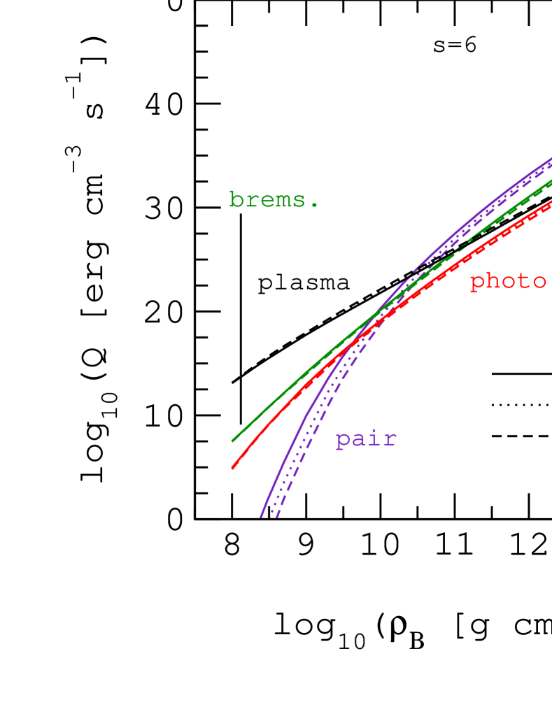
Figure 10: Comparison of neutrino emissivities from the pair, plasma, photo, and bremsstrahlung processes at constant entropies per baryon of $s=4,6,8$, and 10, respectively. The corresponding temperatures are shown in Fig. 9.

Traditionally, comparisons of total emissivities from the various processes have been carried out using $T$ and $\rho_{B}Y_{e}$ as variables. In the context of supernova dynamics, additional insights can be gained by making comparisons along constant entropy per baryon adiabats as a function of baryon density $\rho_{B}$. We therefore present constant entropy per baryon adiabats in Fig. 9. The results in this figure are based on calculations of the equation of state of matter in which the net negative electric charge of electrons and positrons is cancelled by a uniform positively charged background of protons, alpha particles, and heavier ions (see, for example, Ref. LS and references therein). The phase structure of matter and the relative abundances of the various constituents including those of dripped neutrons at sub-nuclear densities are determined by the minimization of free energy.

In Fig. 10, we compare the total neutrino emissivities from the various processes at constant entropy per baryon (in units of $k_{B}$) of $s=4,6,8$ and 10, respectively. The plasma neutrino emissivity dominates over the other processes considered for entropies and densities that lie at the lower ends of those shown in this figure. Toward the higher ends of entropies and densities, the pair and bremsstrahlung processes are far more efficient than both the photo and plasma processes. Once the threshold of $T\sim 2m_{e}$ is crossed, $e^{+}e^{-}$ annihilation becomes the dominant source of $\nu\bar{\nu}$ pairs, the emissivity growing as $T^{9}$. The dominance of the bremsstrahlung process at low entropies and high densities is due to the increasing number of participating Pauli-unblocked nucleon pairs that can benefit from strong interaction (pion-exchange) dynamics. Note that the electron fraction $Y_{e}$ has a significant effect only for the pair emissivity, which depends directly on the number of $e^{+}e^{-}$ pairs, which grows with increasing $s$ (or $T$ at a given density). The plasma and photo processes are much less sensitive to $Y_{e}$, primarily because of the presence of electrons even without positrons. The insensitivity of the bremsstrahlung process to $Y_{e}$ is due to the preponderance of $nn$ pairs under these physical conditions.

The relative importance of the plasma process depends on whether or not favorable conditions are encountered during the course of supernova dynamics. Simulations peformed to date Bruenn93 ; Janka03 point to the low density ($\rho_{B}<10^{11}~{}{\rm g~{}cm^{-3}}$) and low entropy ($s<6$) regions encountered a few tens of milliseconds after bounce. For electron neutrinos and antineutrinos, the pair reactions are only corrections compared to the beta decay and capture processes. For $\mu$ and $\tau$ neutrinos, densities of $\rho_{B}<10^{11}~{}{\rm g~{}cm^{-3}}$ lie below the neutrinosphere located at $\rho_{B}\sim 10^{12}~{}{\rm g~{}cm^{-3}}$. The largest pair rate at the latter density is 5-10 orders larger than the plasma rate in its most relevant region. At $s=4$, plasma neutrinos are, however, competitive with those from pair and bremsstrahlung processes at the neutrinospheric density (but such low entropies in current post bounce models occur only at much higher densities). In order to judge the relative importance for neutrino transport, consult the discussion of thermalization depths for the different processes in Ref. KRJ02 . It must be emphasized, however, that the values of $s,T$ and $\rho_{B}$ attained in such simulations are predicated both by the input microscopic physics and the complex interplay of neutrino transport with hydrodynamics (in many cases coupled with convection, rotation and magnetic fields), both of which are being currently improved. The differential emissivities presented in this work are a part of such improvements in the area of microphysical ingredients and their relative importance remains to be ascertained in the future.

VII Summary and Outlook

In summary,

• We have calculated the differential rates and emissivities of neutrino pairs from an equilibrium plasma for baryon densities $\rho_{B}<10^{14}~{}{\rm g~{}cm^{-3}}$ and temperatures $T\leq 10^{11}$ K. We have checked that the new analytical expressions for the differential emissivities yield total emissivities that are consistent with those calculated using independent methods.

• We have developed new analytical expressions for the total emissivities in various limiting situations. These results help us to better understand qualitatively the scaling of the results with physical quantities such as the chemical potential and plasma frequency at each temperature and density. A comparison with other competing processes, such as $e^{+}e^{-}$ annihilation, $e^{-}\gamma$ interaction, and nucleon-nucleon bremsstrahlung, shows that the plasma process is the dominant source of neutrino pairs in regions of high degeneracy.

• Using our results for the differential rates and emissivities, we have calculated the production and absorption kernels in the source term of the Boltzmann equation employed in exact, albeit numerical, treatments of multi-energy neutrino transport. We have also provided the appropriate Legendre coefficients of these kernels in forms suitable for multi-group flux-limited diffusion schemes.

The significance of neutrino pair production from the plasma process in detailed calculations of core-collapse supernovae in which neutrino transport is strongly coupled with hydrodynamics remains to be explored. The detailed differential information provided in this work may also be of utility in better understanding the evolution of other astrophysical systems such as the red giant stages of stellar evolution, the cooling and accretion-induced collapse of white dwarfs, burning phenomena atop neutron stars, the explosive stages of type Ia supernovae, and gamma-ray bursters.

Appendix A Effective Coupling

The decay of a massive photon or plasmon into a $\nu\bar{\nu}$ pair requires the coupling of the intermediate off-shell $e^{+}e^{-}$ pair to the outgoing neutrinos. Since neutrinos can belong to any of the three flavors, and the loop calculation is performed including the $e^{+}e^{-}$ pair only, different $\nu$ flavors will have different rates of emission due to different couplings to the $e^{+}e^{-}$ pair.

The electron-positron couplings to the neutrino-antineutrino pair described by the two one-loop Feynman diagrams in Fig. 1 are given by the matrix elements:

$$\mathcal{M}_{Z} = \left(\bar{u_{\nu}}\frac{-ig_{Z}}{2}\gamma^{\mu}(c_{V}^{i}-c_{A}^{i}\gamma_{5})v_{\nu}\right)(-i)\frac{g_{\mu\nu}-Q_{\mu}Q_{\nu}/M_{Z}^{2}}{Q^{2}-M_{Z}^{2}}\left(\bar{v_{e}}\frac{-ig_{Z}}{2}\gamma^{\nu}(c_{V}^{e}-c_{A}^{e}\gamma_{5})u_{e}\right)\,,$$ (132)

$$\mathcal{M}_{W} = \left(\bar{u_{\nu}}\frac{-ig_{W}}{2\sqrt{2}}\gamma^{\mu}(1-\gamma_{5})u_{e}\right)(-i)\frac{g_{\mu\nu}-Q_{\mu}Q_{\nu}/M_{W}^{2}}{Q^{2}-M_{W}^{2}}\left(\bar{v_{e}}\frac{-ig_{W}}{2\sqrt{2}}\gamma^{\nu}(1-\gamma_{5})v_{\nu}\right)\,,$$ (133)

where in Eq. (132) the superscript $i$ denotes neutrino flavor. The coefficients $c_{V}$ and $c_{A}$ are:

$$c_{V} = \frac{1}{2}\qquad{\rm and}~{}~{}c_{A}=\frac{1}{2}\qquad{\rm for}~{}~{}\nu_{e},~{}\nu_{\mu}~{}~{}{\rm and}~{}~{}\nu_{\tau}$$

$$c_{V} = -\frac{1}{2}+2\sin^{2}\theta_{W}~{}~{}{\rm and}~{}~{}c_{A}=-\frac{1}{2}~{}~{}{\rm for}~{}~{}e,~{}\mu,~{}{\rm and}~{}\tau\,.$$ (134)

While the exchange of the $Z-$boson produces all three neutrino and antineutrino flavors ($\nu_{e,\mu,\tau}$), $W-$boson exchange produces only $\nu_{e}\bar{\nu}_{e}$ pair. This gives rise to different production rates for different $\nu$ types so that the electron neutrino will have a different emissivity compared to those of the $\nu_{\mu}$ and $\nu_{\tau}$.

It is economical to rephrase these two diagrams into an effective form dependent on the $\nu$ type. After performing Fierz rearrangement and discarding the $Z$ and $W$ momenta ($M_{Z,W}^{2}\gg q^{2}$), we obtain the effective $e^{+}e^{-}$ coupling

$$\mathcal{M}_{eff} = \frac{-iG_{F}}{\sqrt{2}}\big{(}\bar{u_{\nu}}\gamma^{\mu}(1-\gamma_{5})v_{\nu}\big{)}\big{(}\bar{v_{e}}\gamma_{\mu}(C_{V}^{f}-C_{A}^{f}\gamma_{5})u_{e}\big{)}\,,$$ (135)

where the couplings $C_{V}^{f}$ and $C_{A}^{f}$ now depend on the outgoing neutrino flavor. Their numerical values are

$$C_{V} = \frac{1}{2}+2\sin^{2}\theta_{W},\quad C_{A}=\frac{1}{2}\quad{\rm for}~{}\nu_{e}$$

$$C_{V} = -\frac{1}{2}+2\sin^{2}\theta_{W},\quad C_{A}=-\frac{1}{2}\quad{\rm for}~{}\nu_{\mu}~{}{\rm and}~{}\nu_{\tau}\,.$$ (136)

The reduction of the interaction to a single effective interaction significantly simplifies calculations of rates and emissivities from the process $\gamma^{*}\rightarrow\nu+\bar{\nu}$.

References

- (1) A. V. Sweigart and P. G. Gross, Astrophys. Jl. Suppl. Ser. 36, 405 (1978).
- (2) G. G. Raffelt, Phys. Rep. 333, 593 (2000).
- (3) M. S. O’Brien and S. D. Kawaler, Astrophys. J. 539, 372 (2000).
- (4) M. Prakash, J. M. Lattimer, R. F. Sawyer, and R. R. Volkas, Ann. Rev. Nucl. Part. Sci. 51, 295 (2001).
- (5) D. G. Yakovlev, A. D. Kaminker, O. Y. Gnedin, and P. Haensel, Phys. Rep. 354, 1 (2001).
- (6) W. Hillebrandt and J. C. Niemeyer, Ann. Rev. Astron. and Astrophys. 38, 191 (2000).
- (7) K. Iwamoto, et al., Astrophys. Jl. Suppl. Ser. 125, 439 (1999).
- (8) A. Burrows, Nature 403, 727 (2000).
- (9) T. Di Matteo, R. Perna, and R. Narayan, Astrophys. J. 579, 706 (2002).
- (10) K. Kohri and S. Mineshige, Astrophys. J. 577, 311 (2002).
- (11) O. E. B. Messer, A. Mezzacappa, S. W. Bruenn, and M. W. Guidry, Astrophys. J. 507, 353 (1998); S. Yamada, H-Th Janka, H. Suzuki, Astron. Astrophys. 344, 533–550 (1999); A. Burrows, T. Young, P. Pinto, R. Eastman, T. A. Thompson, Astrophys. J. 539, 865 (2000); M. Rampp, H-Th Janka, Astrophys. J. 539, L33 (2000); M. Liebendoerfer, et al. Phys. Rev. D 63, 104003-1 (2001).
- (12) S. W. Bruenn, Astrophys. Jl. Suppl. Ser. 58, 771-841 (1985).
- (13) A. Burrows and T. A. Thompson, astro-ph/0211404
- (14) E. Braaten and D. Segel, Phys. Rev. D 48, 1478-1491 (1993).
- (15) G. Beaudet, V. Petrosian and E. E. Salpeter, Phys. Rev. 154, 1445-1454 (1966).
- (16) G. Beaudet, V. Petrosian and E. E. Salpeter, Astrophys. J. 150, 979-999 (1967).
- (17) D. A. Dicus, Phys. Rev. D 6, 941-949 (1972).
- (18) J. R. Bond, Ph. D. Thesis: Neutrino production and transport during gravitational collapse (California Institute of Technology) 1978.
- (19) P. J. Schinder, D. N. Schramm, P. J. Wita, S. H. Margolis, D. L. Tubbs, Astrophys. J. 313, 531-542 (1987).
- (20) J. I. Kapusta, Finite-temperature field theory (Cambridge University Press) 1989.
- (21) M. Le Bellac, Thermal field theory (Cambridge University Press) 1996.
- (22) E. Braaten, Phys. Rev. Lett. 48, 1655-1658 (1991).
- (23) The polarization vector in Eqs. (24) and (25) is a 4–vector introduced as a part of the orthogonal set . The frequency and wave vector occuring in satisfy the transverse dispersion relation.
- (24) M. Haft, G. Raffelt, A. Weiss Astrophys. J. 425, 222-230 (1994).
- (25) S. Hannestadt and G. Raffelt, Astrophys. J. 507, 339-352 (1998).
- (26) J. M. Lattimer and F. D. Swesty, Nucl. Phys. A 535, 331 (1991).
- (27) S. Bruenn, in Nuclear Physics in the Universe, Edited by M. W. Guidry & M. R. Strayer, Institute of Physics Publishing (Bristol & Philadelphia, 1993), p. 31 (1992-93).
- (28) Private communication.
- (29) M. Th. Keil, G. G. Raffelt, and H-T. Janka, astro-ph/0208035.