Probing the Ionization State of the Universe at $z>6$

Abstract

We present high signal-to-noise ratio Keck ESI spectra of the two quasars known to have Gunn-Peterson absorption troughs, SDSS J1030$+$0524 ($z=6.28$) and SDSS J1148$+$5251 ($z=6.37$). The Ly$\,\alpha$ and Ly$\,\beta$ troughs for SDSS J1030$+$0524 are very black and show no evidence for any emission over a redshift interval of $\sim 0.2$ starting at $z=6$. On the other hand, SDSS J1148$+$5251 shows a number of emission peaks in the Ly$\,\beta$ Gunn-Peterson trough along with a single weak peak in the Ly$\,\alpha$ trough. The Ly$\,\alpha$ emission has corresponding Ly$\,\beta$ emission, suggesting that it is indeed a region of lower optical depth in the intergalactic medium at $z=6.08$.

The stronger Ly$\,\beta$ peaks in the spectrum of SDSS J1148$+$5251 could conceivably also be the result of “leaks” in the IGM, but we suggest that they are instead Ly$\,\alpha$ emission from an intervening galaxy at $z=4.9$. This hypothesis gains credence from a strong complex of C IV absorption at the same redshift and from the detection of continuum emission in the Ly$\,\alpha$ trough at the expected brightness. If this proposal is correct, the quasar light has probably been magnified through gravitational lensing by the intervening galaxy. The Strömgren sphere observed in the absorption spectrum of SDSS J1148$+$5251 is significantly smaller than expected based on its brightness, which is consistent with the hypothesis that the quasar is lensed.

If our argument for lensing is correct, the optical depths derived from the troughs of SDSS J1148$+$5251 are only lower limits (albeit still quite strong, with $\tau(\hbox{Ly$\,\alpha$})>16$ inferred from the Ly$\,\beta$ trough.) The Ly$\,\beta$ absorption trough of SDSS J1030$+$0524 gives the single best measurement of the IGM transmission at $z>6$, with an inferred optical depth $\tau(\hbox{Ly$\,\alpha$})>22$.

1 Introduction

The discovery of quasars at redshifts greater than 6 from the Sloan Digital Sky Survey (SDSS; Fan et al. 2001, Fan et al. 2003) has opened a window for spectroscopic exploration of the high redshift intergalactic medium. The detection of broad, black, Ly$\,\alpha$ absorption troughs, as predicted by Gunn & Peterson (1965; hereafter GP), indicates that we are beginning to probe the era when hydrogen was reionized by an early generation of stars. Becker et al. (2001) detected the first complete GP trough in the spectrum of SDSSp J103027.10$+$052455.0 ($z=6.28$; hereafter SDSS J1030$+$0524). They compared the absorption to that seen in the spectra of lower redshift quasars and concluded that the fraction of neutral hydrogen in the IGM increases sharply at $z\sim 6$. Fan et al. (2003) report that the most distant known quasar, SDSS J114816.64$+$525150.3 ($z=6.37$; hereafter SDSS J1148$+$5251), also shows a complete GP trough in its spectrum. Djorgovski, Castro, Stern & Mahabal (2001) argued that the spectra of even lower redshift quasars show indications of neutral regions in the IGM.

There ensued a spate of theoretical papers discussing the details of how reionization takes place. But the most exciting new observational result is undoubtedly the discovery by the Wilkinson Microwave Anisotropy Probe (WMAP) that the microwave background has traversed a moderate optical depth ($\tau=0.17\pm 0.04$) electron scattering medium, implying that the universe must have been ionized at $z\sim 10$–20 (Kogut et al. 2003). At first glance this appears inconsistent with reionization at $z\sim 6$, but since a relatively small neutral fraction ($\sim 1$%) would suffice to produce black GP troughs, the results are not contradictory. There is mounting evidence that the ionization history of the intergalactic medium (IGM) was complex. Wyithe & Loeb (2003) suggested that the hydrogen in the IGM could have been reionized twice, and Cen (2003) argued that two phases of reionization are likely under a wide range of conditions. In this scenario, the first reionization occurs at $z\sim 15$, driven by the formation of massive, zero-metallicity Population III stars (Venkatesan, Tumlinson & Shull 2003; Mackey, Bromm & Hernquist 2003). The ionizing radiation from massive stars is dramatically reduced, however, when Pop III supernovae seed the gas with metals (due to a reduction in the formation of massive stars, increased line-blanketing in hot star atmospheres, and increased mass loss rates from both hot stars and red giants.) Consequently the IGM recombines and remains relatively neutral, $n_{\rm HI}/n_{\rm H}>0.1$, until an increasing Pop II massive star population and a declining IGM density allow the second reionization to occur at $z\sim 6$. This neutral fraction is sufficient to produce the observed high optical depths in the Ly$\,\alpha$ GP troughs of high redshift quasars.

To advance our understanding of the ionization history of the universe, we need high resolution, high signal-to-noise ratio spectra of the IGM absorption at $z>6$. Recently several groups have discovered Ly$\,\alpha$-emitting galaxies at $z\sim 6.5$ (Hu et al. 2002, Kodaira et al. 2003). These objects are interesting and relevant as direct probes of star and galaxy formation at $z>6$, and the mere detectability of their Ly$\,\alpha$ emission is an important clue to the ionization state of the IGM (Haiman 2002). However, their continua are far too faint (even redward of Ly$\,\alpha$) to make them useful for studies of the intervening IGM. Only high-redshift quasars offer the possibility of acquiring high quality information on the state of the IGM at high redshift.

In this paper we present high quality spectra of the only two quasars known to have GP absorption troughs, SDSS J1030$+$0524 ($z=6.28$) and SDSS J1148$+$5251 ($z=6.37$), taken with the ESI spectrograph on the Keck Telescope. The following sections describe the observations and data reduction (§2), discuss the analysis methods used (§3), present the properties of the IGM absorption in the spectra (§4), and discuss the results (§5). Appendix A explores the effect of light travel time on the observed expansion of ionization fronts around high-redshift quasars.

2 Observations

Spectra of SDSS J1030$+$0524 and SDSS J1148$+$5251 were taken with the Keck Echellette Spectrograph and Imager (ESI; Sheinis et al. 2002) between January 2002 and February 2003. ESI covers the wavelength range 4000–11000 Å with 10 Echelle orders having a constant resolution of $R=\lambda/\Delta\lambda\sim 10000$ ($\sim 30$ km/s). The data were taken with the slit at the parallactic angle in mostly good but variable seeing (from 0.6″ to $>1$″, with mean seeing around 0.8″). The sky transparency ranged from photometric to light cirrus. A log of the observations is given in Table 1.

Table 1: Keck ESI Observation Log

Source	Date	Slit Width	Number of	Total Exposure
	yyyy/mm/dd	(″)	Exposures	(hr)
SDSS J1030$+$0524	2002/01/10	1.00	6	2.00
SDSS J1030$+$0524	2002/01/11	1.00	5	1.67
SDSS J1030$+$0524	2002/01/12	1.00	12	4.00
SDSS J1030$+$0524	2002/01/13	0.75	2	1.50
SDSS J1030$+$0524	2002/02/07	0.75	2	1.50
SDSS J1148$+$5251	2002/12/04	1.00	9	3.00
SDSS J1148$+$5251	2002/12/05	1.00	10	3.33
SDSS J1148$+$5251	2003/02/04	1.00	14	4.67

The most challenging data reduction problem for these observations is subtracting the sky background, including the bright OH lines that dominate the near infrared atmospheric emission. The sky is considerably brighter than the object, and small errors in the sky subtraction can easily produce offsets in the emission that either create the appearance of light in the absorption trough or remove light that should be present there. To assist in the sky subtraction, we shifted the object along the slit for the various integrations, which helps to average over any small-scale flat-fielding, bias or dark current variations not corrected by the standard CCD calibrations.

The sky brightness varies as a function of time in a complex way in the near infrared, with the atmospheric OH emission varying rapidly and independently of other sky emission. In addition the ESI spectrograph, though a highly stable instrument, does undergo small changes over time, with the wavelengths shifting slightly from one observation to the next. Presumably these changes (which are typically at the level of a few tenths of a pixel or less) are due to minor thermal and gravity-induced flexures.

We extract a sky-subtracted spectrum from each independent observation. The separate spectra are then combined using weights to optimize the signal-to-noise ratio of the result. It is necessary to be very careful with the weights for combining to avoid any bias in the results. A simple unweighted average is safely free of bias but leads to a much noisier spectrum than an optimally weighted sum. On the other hand, using weights $1/\sigma^{2}$ with $\sigma$ derived from the noise estimates of the individual spectra leads to a very noticeable bias toward lower flux values, because the estimated noise is larger for brighter pixels. In the black absorption troughs this leads to fluxes that are systematically negative.

The dangers of using a weighted combination for Poisson data are well-documented (for a nice analysis, see Wheaton et al. 1995). The cure for the bias is to choose weights that are completely independent of the data. We have combined the spectra using weights that are derived from the sky noise in adjacent pixels (i.e., along the slit). Note that using the sky noise from the same pixel would still lead to a small bias, because pixels that have positive sky fluctuations (making the residual counts a little low) would be given slightly lower weights, thus leading to a positive bias in the sum. Using the sky noise in neighboring pixels produces a completely unbiased result that has a nearly optimal signal-to-noise ratio. An overall scale factor is determined for each spectrum to match the fluxes, thereby correcting for variable atmospheric transparency.

Our extraction algorithm is highly customized for ESI data, which have a number of unusual characteristics (e.g., highly curved orders, a strongly non-linear wavelength dispersion, and some odd notches in the sensitivity in the bluer orders.) The images are first geometrically rectified to produce orders with orthogonal wavelength and spatial coordinates lying along rows and columns. This removes the very large curvature of the ESI Echelle orders and also corrects small variations in the wavelength dispersion along the slit that manifest themselves as tilted or curved sky lines. The order curvature removal also automatically corrects the spectral trace for differential atmospheric refraction using the airmass of the observation; this approach is more effective than tracing the orders directly because high-redshift quasar spectra have long stretches with no detectable light, foiling standard tracing algorithms.

The resampling algorithm used in the rectification is a flux-conserving interpolation scheme that is accurate to second order in the pixel shifts (as opposed to the more commonly used schemes that are only first order, making them considerably more dispersive.) The interpolation method is based on the high-order, monotonic, flux-conserving advection schemes that are widely used in modern hydrodynamic simulations (van Leer 1977).

Extraction of spectra from the rectified orders is straightforward. We use an optimal extraction algorithm with a second-order fit to the sky along the slit and a spatial profile that is assumed constant for each order. For orders where the profile is not detected, the trace position and width are predicted based on those orders that are detected. The wavelength scale derived from calibration lamps is adjusted using the positions of sky lines for each observation. The final spectra for the quasars are shown in Figure 1.

Figure 1: Keck ESI spectra of the two highest redshift quasars. The spectra have been binned to a resolution $R=\Delta\lambda/\lambda=2500$ (120 km/s). The Gunn-Peterson absorption troughs of Ly$\,\alpha$ and Ly$\,\beta$ are indicated, extending from $z=5.975$ to 6.165 (SDSS J1030$+$0524) and $z=6.075$ to 6.320 (SDSS J1148$+$5251).

3 Analysis of the Spectra

High signal-to-noise ratio spectra promise two improvements in our understanding of the GP troughs. By reducing the noise in the black regions of the spectrum, they improve our lower limits on the absorbing optical depth and may allow us to detect faint light in the dark troughs. But since the optical depth limits increase only as the logarithm of the signal-to-noise ratio, which itself increases only as the square root of the integration time, it is difficult to make dramatic improvements in the limits. The main benefit of high signal-to-noise ratio spectra is that they allow us to set strong detection limits over narrower bands in the spectra. The optical depth distribution is very unlikely to be a smooth function of redshift; instead, at the transition between a neutral and an ionized IGM, there will be ionized, partially transparent bubbles sprinkled along the line of sight. To detect these bubbles we need to be able to recognize narrow emission spikes in the trough where the quasar light leaks through the IGM. The new spectra presented in the paper are far better for that purpose than our earlier observations (which were 30 min exposures taken with ESI.)

We begin with an approach similar to that used by Becker et al. (2001). The residual fluxes in the GP troughs of Ly$\,\alpha$ and Ly$\,\beta$ are measured directly from the spectra; the fluxes are weighted using the sky noise from adjacent pixels (as described above for the extraction) to improve the signal-to-noise ratio while avoiding bias in the sums. Then the mean transmission and optical depth of the IGM are determined by comparing the residual flux to the (unabsorbed) quasar continuum at the positions of the troughs.

Because very little neutral hydrogen is required to create a GP trough in Ly$\,\alpha$ (a 1% neutral fraction will suffice), the presence of a GP trough due to Ly$\,\alpha$ provides only a lower limit to the amount of neutral hydrogen. The GP trough from the Ly$\,\beta$ transition can be a more sensitive test because the Ly$\,\beta$ cross-section is a factor of 5.27 lower than Ly$\,\alpha$. Interpretation of the Ly$\,\beta$ trough is complicated by the fact that it is overlaid by the Ly$\,\alpha$ forest at $z\sim 5$, which is unpredictable along a given line of sight due to cosmic variance. In spite of that, using fairly secure assumptions, the Ly$\,\beta$ trough can give much stronger limits on the neutral hydrogen fraction. We consequently measure residual fluxes in both the Ly$\,\alpha$ and Ly$\,\beta$ absorption regions.

We also considered using the Ly$\,\gamma$ absorption since Ly$\,\gamma$ has an even lower intrinsic optical depth. However, the Ly$\,\gamma$ GP trough suffers from overlying absorption by both Ly$\,\alpha$ and Ly$\,\beta$ at lower redshifts and consequently does not give additional useful information.

It is necessary to estimate the brightness of the quasar continuum at the Ly$\,\alpha$ and Ly$\,\beta$ troughs in order to measure the transmission of the IGM. For this purpose we use the far UV quasar power law spectrum of Telfer, Zheng, Kriss, & Davidsen (2002) and the composite spectrum from the Large Bright Quasar Survey (LBQS; Francis et al. 1991). The templates are matched to the observed spectra at a rest wavelength of $\sim 1290$ Å. The Telfer et al. power law has a break near 1280 Å and rises less steeply into the UV than a simple extrapolation of the continuum redward of Ly$\,\alpha$. In the near UV ($\lambda>1280$ Å), the spectral slope is $\alpha_{NUV}=-0.72$ ($f_{\nu}\propto\nu^{\alpha}$), while in the far UV ($\lambda<1280$ Å), $\alpha_{EUV}=-1.57$ for radio-quiet objects and $-1.96$ for radio-loud objects. While there is no evidence that either of our quasars is radio-loud, we compute continuum levels using both EUV slopes in order to represent the range of continua seen in quasars.

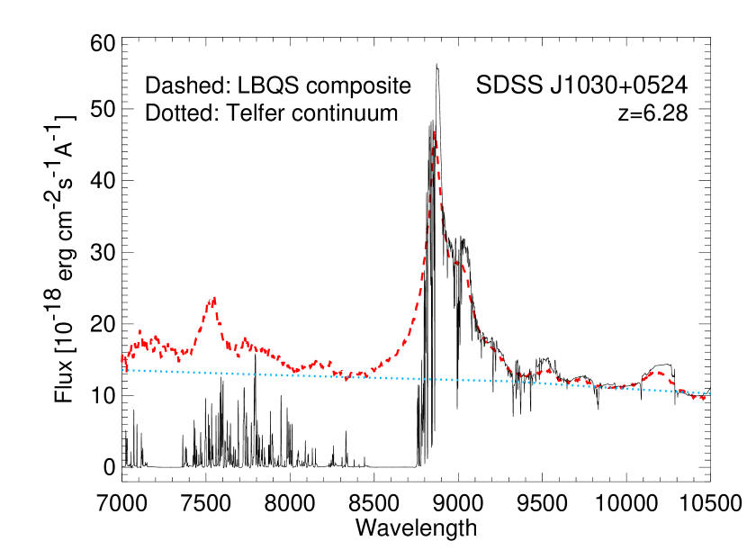
Figure 2: Denoised, full-resolution spectrum of SDSS J1030$+$0524 with matched templates from the LBQS and Telfer et al. (2002). The denoising algorithm is described in the text. The template is a very good match to the quasar redward of the Ly$\,\alpha$ IGM absorption.

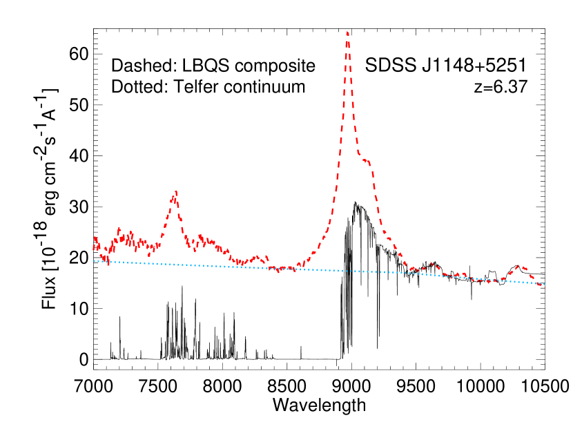
Figure 3: Denoised, full-resolution spectrum of SDSS J1148$+$5251 with matched templates from the LBQS and Telfer et al. The hydrogen emission lines are much weaker than those in the template. Our best redshift determination for this object, $z=6.37$, comes from matching the features redward of 9500 Å with the template.

Broad emission lines can also contribute to the continuum. Our spectra are displayed in Figures 2 and 3 along with the LBQS composite spectrum. For these figures, our spectra have been denoised using a wavelet shrinkage algorithm (Donoho & Johnstone 1994) that is optimized for the case where the noise amplitude is variable but known (heteroscedastic data, in the parlance of statisticians). We use a Haar (1910) wavelet transform, which allows error propagation and has the great benefit of keeping the noise in transform space uncorrelated at each scale before the filtering is applied. Cycle-spinning (Coifman & Donoho 1995) is utilized to make the result shift-invariant and to remove the artifacts generated by the square-wave Haar basis functions.

Denoising thus uses a variable smoothing length to suppress the noise as much as possible on all scales while remaining consistent with the spectrum given the estimated noise array. The resulting spectrum is heavily smoothed in flat regions (such as the dark troughs), which suppresses the noise. (Values in the smoothed areas are consequently highly correlated.) The smoothing threshold is set to $3\sigma$, so only structures more significant than that remain in the spectrum. Note that high resolution structures are preserved (compare the absorption on the blue edge of the Ly$\,\alpha$ emission with Fig. 1) while the noise in both the continuum and the troughs is dramatically reduced.

For SDSS J1030$+$0524 (Fig. 2), the LBQS composite is clearly a good match to the spectrum, so we estimate the continuum in the Ly$\,\alpha$ and Ly$\,\beta$ absorption troughs using the mean flux in the relevant wavelength window from the LBQS spectrum. On the other hand, SDSS J1148$+$5251 shows considerably weaker emission lines than the composite (Fig. 3); we therefore use the Telfer et al. power law continuum alone as the estimate of the brightness at the absorption troughs. The continua estimated by using these different templates differ by about 30%.

4 Results

4.1 SDSS J1030$+$0524

For SDSS J1030$+$0524, our results can be described very simply: the GP absorption troughs of both Ly$\,\alpha$ and Ly$\,\beta$ are very black. There is no evidence of any residual light in the troughs to the limit of our observations. The Ly$\,\alpha$ and Ly$\,\beta$ absorption trough details are shown in Figure 4.

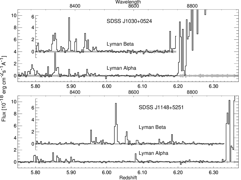
Figure 4: Closeup of the Ly$\,\alpha$ and Ly$\,\beta$ GP troughs, aligned in redshift, at a resolution of $R=2500$ (120 km/s). Note that these spectra have not been denoised, so the pixel values are independent. The top axis shows the wavelength for Ly$\,\alpha$, and the shaded band shows $1\sigma$ errors. The absorption is extraordinarily black for SDSS J1030$+$0524, but SDSS J1148$+$5251 shows evidence for weak emission in the trough, especially at Ly$\,\beta$. The strong peaks in the Ly$\,\beta$ spectrum at $z=6.02$ and 6.06 are discussed in the text; they could be Ly$\,\alpha$ emission from a foreground galaxy at $z=5$.

Table 2: Absorption Properties of $z>6$ Quasars

Object	GP Trough	$\lambda_{min}$	$\lambda_{max}$	$z_{min}$	$z_{max}$	Residual Flux	Continuum	IGM Transmission	Ly$\,\alpha$ Optical
		(Å)	(Å)			($10^{-20}\,\hbox{erg}\,\hbox{s}^{-1}\hbox{cm}^{-2}\hbox{\AA}^{-1}$)		Fraction	Depth
SDSS J1030$+$0524	Ly$\,\alpha$	8510	8710	6.00	6.17	$1.6\pm 1.4$	1570	$0.0010\pm 0.0009$	$>6.3$
$z_{em}=6.28$	Ly$\,\beta$	7180	7349	6.00	6.17	$0.8\pm 1.7$	200	$0.0043\pm 0.0088$	$>22.8$
SDSS J1148$+$5251	Ly$\,\alpha$	8630	8900	6.10	6.32	$3.6\pm 0.8$	1730	$0.0021\pm 0.0005$	$6.2\pm 0.2$
$z_{em}=6.37$	Ly$\,\beta$	7282	7509	6.10	6.32	$9.6\pm 1.0$	210	$0.0465\pm 0.0047$	$16.2\pm 0.6$
	Ly$\,\beta$	7282	7509	6.10	6.32	$9.6\pm 1.0$	190	$0.0510\pm 0.0052$	$15.7\pm 0.6$
	Ly$\,\alpha$	8510	8630	6.00	6.10	$10.9\pm 1.1$	1740	$0.0063\pm 0.0007$	$5.1\pm 0.1$
	Ly$\,\beta$	7180	7282	6.00	6.10	$63.4\pm 1.4$	210	$0.3020\pm 0.0067$	$6.3\pm 0.1$
	Ly$\,\beta$	7180	7282	6.00	6.10	$63.4\pm 1.4$	190	$0.3350\pm 0.0074$	$5.8\pm 0.1$

The results are summarized in Table 2. The band limits were chosen to exclude the first bright peaks on either end of the Ly$\,\beta$ GP trough and are identical in redshift for the two troughs. The residual fluxes for both the Ly$\,\alpha$ and Ly$\,\beta$ troughs are consistent with zero.

For the Ly$\,\beta$ trough, the continuum estimate includes a reduction factor of 0.12 for the overlying Ly$\,\alpha$ forest absorption at $z=5$ (as determined by Becker et al. 2001) The $\tau(\hbox{Ly$\,\beta$})$ values are converted to equivalent Ly$\,\alpha$ optical depths by multiplying by 5.27, the ratio of the oscillator strengths of the two lines. Thus the Ly$\,\beta$ GP trough measurements for SDSS J1030$+$0524 imply $\tau(\hbox{Ly$\,\alpha$})>22.8$ ($1\sigma$). The errors quoted in the table reflect only the statistical uncertainties. As found by Becker et al., the strongest limit on the optical depth comes from the Ly$\,\beta$ trough, despite the additional uncertainty that comes from the overlying Ly$\,\alpha$ absorption.

These results are consistent with the measurements of Becker et al. (2001) (confirmed by Pentericci et al. 2002) but are naturally stronger given the much improved signal-to-noise ratio of the data. Our limits on the residual flux in the GP troughs and the Ly$\,\alpha$ optical depth of the IGM are lower by the expected factors given the longer integrations reported here. The limits remain consistent with zero flux in the GP troughs of SDSS J1030$+$0524.

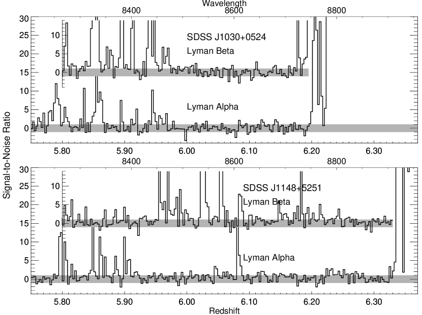
Figure 5: Signal-to-noise ratios for the Ly$\,\alpha$ and Ly$\,\beta$ absorption troughs in SDSS J1030$+$0524 and SDSS J1148$+$5251.

There is no evidence for any significant peaks in either trough. Figure 5 displays the signal-to-noise ratio of the spectra in the troughs. The distribution is consistent with zero-mean noise in the troughs; the reduced $\chi_{\nu}^{2}$ for the combined Ly$\,\alpha$ and Ly$\,\beta$ troughs is 0.97.

4.2 SDSS J1148$+$5251

The GP troughs for SDSS J1148$+$5251 are also shown in Figures 4 and 5. The mean transmission properties of the troughs are given in Table 2, which includes the transmission measured for both a high redshift range ($6.1<z<6.32$) and a lower redshift interval ($6.0<z<6.1$). Note that we now quote a measurement, not a lower limit, on $\tau$, as flux has been detected in the troughs. The correction factor for Ly$\,\alpha$ forest absorption overlying the Ly$\,\beta$ GP trough was taken to be 0.11, from Figure 2 of Becker et al. (2001). The $1\sigma$ errors on the transmission are smaller than for SDSS J1030$+$0524, both because the seeing and photometric conditions were slightly better for SDSS J1148$+$5251 and because its continuum is brighter.

In contrast to SDSS J1030$+$0524, there is light detected in the GP troughs of SDSS J1148$+$5251 both in narrow spikes and in broader bands. The mean transmission nonetheless remains low. Figure 6 summarizes the Ly$\,\alpha$ optical depth as a function of redshift, including additional high-redshift quasars from Fan et al. (2001). There is a noticeable steepening of the $\tau(z)$ relationship at $z\sim 5.8$.

Figure 6: Ly$\,\alpha$ optical depth as a function of redshift from high-redshift quasars. Error bars (and the lower limit for SDSS J1030$+$0524) are $2\sigma$. Data for SDSS J1030$+$0524 and SDSS J1148$+$5251 are from this paper; other data are from Fan et al. (2001). The line shows the expected evolution when the density of Ly$\,\alpha$ forest clouds scales as $(1+z)^{5/2}$ (also from Fan et al.) The implied $\tau(\hbox{Ly$\,\alpha$})$ values from the Ly$\,\beta$ GP trough transmission are substantially stronger: $\tau>22$ (SDSS J1030$+$0524) and $\tau=16$ (SDSS J1148$+$5251). We believe that highest redshift bins for SDSS J1148$+$5251 are probably contaminated by light from an intervening galaxy and so should be considered lower limits.

A closer examination of the troughs reveals some interesting features. The Ly$\,\alpha$ trough extends from $z=5.93$ to 6.32 and looks dark at high resolution except for a weak emission spike at $z=6.08$. The reality of that peak is supported by its coincidence with a Ly$\,\beta$ emission peak at the same redshift (Fig. 4). We believe this is likely to be a real detection of an ionized bubble in the IGM that permits quasar light to leak through at the redshift of the bubble; this feature is discussed in detail below (§5.1).

Several emission spikes are detected in the Ly$\,\beta$ trough as well. Two especially strong peaks are seen at 7205 Å and 7236 Å (Ly$\,\beta$ redshifts of $z=6.03$ and 6.06). There also is significant non-zero flux in the troughs even between the peaks (best seen in Fig. 5). If this flux is quasar light transmitted by the IGM, it certainly suggests strongly that the IGM is not very neutral at $z\sim 6$. That interpretation is not so clear cut, however. We argue below (§5.2) for the alternative interpretation that both the Ly$\,\alpha$ and Ly$\,\beta$ troughs are contaminated by light from an intervening galaxy at $z=5$. If that suggestion is correct, the optical depths derived from the troughs of SDSS J1148$+$5251 are only lower limits.

5 Discussion

5.1 The $z=6.08$ emission feature in SDSS J1148$+$5251

The universe at $z\sim 6$ was very likely ionized by galaxies rather than by quasars, since there do not appear to be enough quasars to do the job (Fan et al. 2001). There must have been regions in the preionized universe where a concentration of unusually luminous galaxies (possibly the precursor to a massive cluster) was capable of ionizing the nearby IGM, creating an ionized bubble. It is therefore not surprising to find weak emission spikes embedded in the mostly black GP troughs (Figs. 4 and 5) where the line-of-sight to the quasar passes through small “holes” in the IGM Ly$\,\alpha$ and Ly$\,\beta$ transmission created by ionized bubbles. That can also explain the detection of Ly$\,\alpha$-emitting galaxies at $z\sim 6.5$ (Hu et al. 2002, Kodaira et al. 2003), which in this picture ought to be found in concentrations with other galaxies.

According to the scenario presented by Cen (2003), the universe is first ionized at $z\sim 15$ by Pop III stars and then recombines to become substantially neutral, with neutral fractions remaining above 0.1 until the second reionization occurs at $z\sim 6$. At $z=6$ to 7 the neutral fraction $n_{\rm HI}/n_{\rm H}$ is typically $\sim 0.15$. As Cen points out, that makes it easier to detect high redshift galaxies; it also makes it easier for lower luminosity sources to create ionized bubbles.

The peak seen in the Ly$\,\alpha$ trough of SDSS J1148$+$5251 at 8600 Å ($z=6.08$) has an intensity about 8% of the extrapolated (pre-absorption) continuum, implying an IGM optical depth of $\tau(\hbox{Ly$\,\alpha$})=2.5$. The optical depth of this window at Ly$\,\beta$ would be only about 0.5, which would produce a very strong peak in the Ly$\,\beta$ trough; but since the overlying Ly$\,\alpha$ forest absorption is expected to reduce that by a factor of 0.11 (corresponding to an overlying optical depth $\tau=2.2$), the expected amplitude of the Ly$\,\beta$ trough peak is in fact very similar to that observed, albeit with a rather large uncertainty in the Ly$\,\alpha$ forest attenuation.

How large would an ionized region need to be to produce this feature? The damping wings from neutral hydrogen on either side of the ionized bubble create a high optical depth through the region unless the bubble is relatively large. This led Barkana (2002) to question Djorgovski et al.’s (2001) argument that dark regions in the spectrum of a lower redshift were created by neutral regions of the IGM. Miralda-Escudé (1998; see also Barkana 2002) derived the Ly$\,\alpha$ damping wing optical depth for hydrogen extending from $z_{1}$ to $z_{2}$ when observed at a wavelength $\lambda_{\alpha}(1+z)$:

$$\tau_{\rm damp}=6.43\times 10^{-9}\,\tau_{\rm GP}\,\left(n_{\rm HI}\over n_{\rm H}\right)\times\left[I\left(1+z_{2}\over 1+z\right)-I\left(1+z_{1}\over 1+z\right)\right]\quad,$$ (1)

where $\tau_{\rm GP}$ is the Gunn-Peterson optical depth,

$$\tau_{\rm GP}=3.42\times 10^{5}\left(1+z\over 7.08\right)^{3/2}\quad,$$ (2)

and we are using a $\Lambda$ cosmology with $H_{0}=70$, $\Omega_{\Lambda}=0.7$, $\Omega_{m}=0.3$, and $\Omega_{b}=0.04$. The function $I(x)$ is defined to be

$$I(x)=x^{1/2}\left({x^{4}\over 1-x}+{9\over 7}x^{3}+{9\over 5}x^{2}+3x+9\right)-{9\over 2}\ln\left|1+x^{1/2}\over 1-x^{1/2}\right|\quad.$$ (3)

Given an ionized region at redshift $z$, Eqn. (1) allows us compute the combined damping wing optical depth from the neutral regions on either side of the bubble. Although the constant factor multiplying $\tau_{\rm GP}$ in Eqn. (1) is small, the leading term in $I(x)$ can be very large near $z=z_{1}$ or $z_{2}$, so $\tau_{\rm damp}$ can be substantial.

Figure 7: Optical depth from damping wings of Ly$\,\alpha$ as a function of diameter for an ionized bubble at $z=6.08$. For small bubbles in a completely neutral IGM (solid line), the damping wings strongly suppress the transmission. If the IGM is already partly ionized ($n_{\rm HI}/n_{\rm H}=0.15$; dashed line) then the optical depths are smaller by the same factor. The dots show the bubble diameter required to produce the observed peak in the Ly$\,\alpha$ trough of SDSS J1148$+$5251 (1.33 Mpc for a neutral IGM or 0.22 Mpc for a partially ionized IGM.)

Figure 7 displays the resulting optical depth for a bubble located at $z=6.08$. The neutral IGM is assumed to extend from $z=6$ to $z=6.32$, but the results are relatively insensitive to those limits. The bubble diameter required to produce a window with $\tau=2.5$ is 1.33 Mpc if the IGM is completely neutral outside the bubble. If the IGM is already partly ionized, the required bubble size is much smaller (0.22 Mpc if $n_{\rm HI}/n_{\rm H}=0.15$).

Barkana (2002) computed the diameter of an H II bubble as a function of the halo mass $M$ of the ionizing source (including the escape probability for ionizing photons in a low metallicity galaxy) to be

$$D_{S}=0.150\,{\rm Mpc}\,\left(7.08\over 1+z\right)\left({N_{\rm ion}\over 20}{M\over 10^{9}\,{\rm M}_{\sun}}\right)^{1/3}\quad,$$ (4)

where $N_{\rm ion}$ is the number of ionizing photons per baryon that escape the galaxy. We can invert this to get the mass required to produce a bubble of a given diameter:

$$M=7\times 10^{11}\,{\rm M}_{\sun}\left({D_{S}\over 1.33\,{\rm Mpc}}{1+z\over 7.08}\right)^{3}{20\over N_{\rm ion}}\quad.$$ (5)

We conclude that a plausible star-forming galaxy (or group of galaxies) along the line of sight can produce the observed peak at $z=6.08$ in the Ly$\,\alpha$ and Ly$\,\beta$ GP troughs of SDSS J1148$+$5251, even if the surrounding IGM is completely neutral. Obviously if the IGM is partly ionized, the required bubble diameter would be much smaller (Fig. 7) and so the required galaxy mass would also be far smaller ($<10^{9}\,{\rm M}_{\sun}$). With future instrumentation it will be interesting to search the vicinity of the quasar for evidence of star-forming galaxies at $z=6.08$ that are the source of the ionizing continuum radiation required to make this bubble.

5.2 Evidence for an intervening $z=5$ galaxy

The strong spikes seen in the Ly$\,\beta$ trough of SDSS J1148$+$5251 at 7205 Å and 7236 Å are more difficult to explain as the result of ionizing bubbles in the IGM. The strength of these peaks is not easily reconciled with the absence of corresponding Ly$\,\alpha$ peaks, given the expected overlying Ly$\,\alpha$ forest absorption. The peak at 7205 Å has an amplitude $8.7\pm 0.3$ ($\times 10^{-18}\,\hbox{erg}\,\hbox{s}^{-1}\hbox{cm}^{-2}\hbox{\AA}^{-1}$), while the brightest plausible continuum at that wavelength is 24 (from the LBQS template spectrum in Fig. 3). If we assume that the 7205 Å peak is quasar light leaking through the $z{=}6$ Ly$\,\beta$ and $z{=}5$ Ly$\,\alpha$ absorption, the implied combined optical depth is $\tau(\hbox{Ly$\,\alpha$@}z{=}5)+\tau(\hbox{Ly$\,\beta$@}z{=}6)=1.0$. But there is no hint of a Ly$\,\alpha$ peak at 8539 Å: the flux limit there is $0.1\pm 0.2$ with an estimated continuum level of 17, implying $3\sigma$ upper limits $\tau(\hbox{Ly$\,\alpha$@}z{=}6)>3.3$ and $\tau(\hbox{Ly$\,\beta$@}z{=}6)=\tau(\hbox{Ly$\,\alpha$@}z{=}6)/5.27>0.6$. The overlying Ly$\,\alpha$ forest absorption must then be $\tau(\hbox{Ly$\,\alpha$@}z{=}5)<0.4$.

We conclude that if the 7205 Å peak is the result of an ionized bubble at $z=6.03$, it must fall in a highly transparent window in the $z=5$ Ly$\,\alpha$ forest that barely attenuates the continuum at all, allowing $>65$% of the light through. High resolution spectra of the Ly$\,\alpha$ forest at $z\sim 5$ (Songaila, Hu, Cowie & McMahon 1999; Djorgovski et al. 2001; Songaila & Cowie 2002) do show small transparent windows, but they are rare. The spectra presented in this paper are typical. There is one transparent window seen at 7800 Å ($z=5.4$) in our spectrum of SDSS J1030$+$0524 (Fig. 2), and no windows at all are seen in SDSS J1148$+$5251. In the $5<z<5.5$ Ly$\,\alpha$ forest, only 0.5% of the bandpass has optical depths less than 0.4. Songaila & Cowie (2002) discuss the distribution of the transmitted fraction as a function of redshift; using their analytical model, at $z=5$ only 1.7% of the spectrum is expected to have a transmission $>0.65$. This fraction drops to only 0.6% if we use the $1\sigma$ upper limit, $\tau(\hbox{Ly$\,\alpha$@}z{=}5)<0.2$.

We conclude that it is problematic to reconcile the strong peak at $z\sim 6.03$ in the Ly$\,\beta$ trough with the absence of a corresponding Ly$\,\alpha$ peak. Unless the Ly$\,\alpha$ forest is extraordinarily transparent at the position of the peak, we would expect a strong, easily detected peak in the Ly$\,\alpha$ GP trough.

There is, however, another possible explanation for the strong peaks in the Ly$\,\beta$ trough of SDSS J1148$+$5251. A careful examination of the quasar spectrum (Fig. 8) reveals a strong C IV absorption feature at 9200A ($z=4.943$). That suggests a second interpretation for the spikes, namely that they are Ly$\,\alpha$ emission from a foreground galaxy at $z=4.943$. Usually one does not see emission associated with C IV absorbers; but ordinarily such emission lines would be lost in the Ly$\,\alpha$ forest and not noticed. This particular emission line, falling as it does in the Ly$\,\beta$ trough, stands out like a sore thumb. Moreover there are multiple C IV absorption systems and multiple (putative) Ly$\,\alpha$ emission components seen, suggesting the presence of a fairly massive mass concentration.

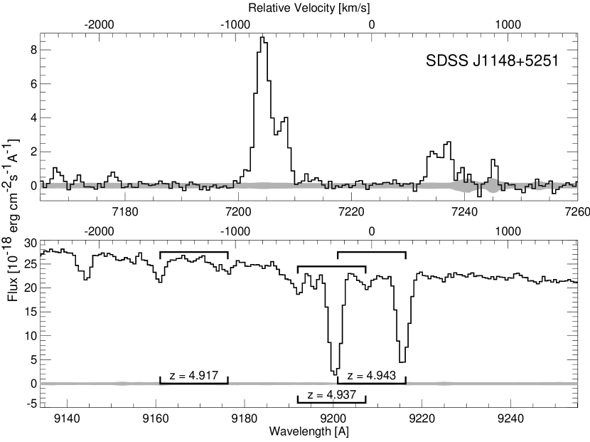
Figure 8: Comparison of emission in the Ly$\,\beta$ GP trough of SDSS J1148$+$5251 with absorption by the C IV 1548.20, 1550.77 doublet, under the assumption that the emission lines are Ly$\,\alpha$ from an intervening galaxy at the same redshift as the C IV absorption, $z=4.943$. Probable C IV absorption systems (having both the correct separation and the correct optical depth ratio) are marked by brackets in the lower panel. The panels are aligned in redshift so that the Ly$\,\alpha$ peak would fall midway between the C IV doublet components for perfect alignment. The velocity axis is registered to the strongest C IV at $z=4.943$. The data are shown at the full resolution of ESI (a substantially higher resolution than is shown in Fig. 4.)

Is it plausible that the emission in the Ly$\,\beta$ trough could be from an intervening $z=4.9$ galaxy? The implied Ly$\,\alpha$ luminosities are similar to those of Ly$\,\alpha$ emitters detected in the Subaru deep field at $z=4.86$ (Ouchi et al. 2003). Moreover, the velocity offset between the Ly$\,\alpha$ emission and the C IV absorption seen in Fig. 8 is in the range typically observed for systems that show both Ly$\,\alpha$ emission and metal line absorption ($\sim 500$ km/s, Shapley et al. 2002).

The main argument against the intervening emission model is that Ly$\,\alpha$ emitters are sufficiently rare on the sky that it is unlikely to find one along a random line-of-sight. But perhaps this is not a random line-of-sight. Figure 8 shows that there are both multiple Ly$\,\alpha$ emission components and multiple C IV absorption components present in the spectrum (note particularly the structure in both components of the strong C IV doublet at 9200 Å.) The two presumed Ly$\,\alpha$ lines are split by 1200 km/s, and the C IV structure extends over at least 250 km/s. It is possible that there is a massive structure (a protocluster?) along the line-of-sight that is amplifying the quasar through gravitational lensing. If that is correct, then the likelihood of finding a Ly$\,\alpha$ emitter in front of the $z=6.37$ quasar is in fact not so small, since the foreground object assisted in the discovery of the quasar by boosting its apparent brightness. Even lensing by a factor of two might create a strong discovery bias since the luminosity function is steep for bright quasars (Wyithe & Loeb 2002; Comerford, Haiman & Schaye 2002).

For the more familiar case where a nearby ($z<1$) galaxy is lensing a high-redshift quasar, the lensing magnification is limited to less than $\sim 2$ because stronger lensing produces multiple images with a noticeably wide splitting. But when the lens redshift is $z\sim 5$, as in the scenario proposed here, the Einstein ring radius is much smaller and so the splitting could not have been detected from the ground (in agreement with the imaging observations by Fan et al. 2003.) Figure 9 shows the magnification and observed image positions as a function of impact parameter for a singular isothermal sphere galaxy model with a velocity dispersion of 250 km/s. This velocity dispersion is consistent with the velocity structure seen in the strong C IV absorption system and is slightly larger than the dispersion expected for an $L_{*}$ galaxy ($v=220$ km/s). In this geometry, the multiple image separation is only 0.3 arcsec, which would be difficult to detect even if the components were of equal brightness.

Figure 9: Gravitational lensing magnification (top) and splitting (bottom) of multiple components for a singular isothermal sphere with a velocity dispersion of 250 km/s. The solid line shows the primary, brighter component; the fainter second image that appears for impact parameters less than the Einstein radius is shown with a dashed line. The total magnification when the two components are combined is shown with a dotted line. Note that the Einstein ring radius is quite small for a quasar at $z=6.4$ being lensed by a galaxy at $z=5.0$, so even high magnification factors are not ruled out by the absence of multiple components in the image.

Note also that since there are multiple C IV absorption and Ly$\,\alpha$ emission components, it is possible that there are multiple lensing galaxies along the line-of-sight to this source. That could possibly increase the amplification factor further, although it would also lead to larger splitting and shifts. We coadded the two-dimensional spectra of SDSS J1148$+$5251 for the Echelle order that includes the Ly$\,\beta$ trough to search for evidence that the peaks are either broader than the quasar trace or are shifted relative to the center of the trace. Neither effect was seen. The width of the peaks agrees with the width of the rest of the order, and the central positions agree to better than 0.1″ (which is the approximate uncertainty in the trace position.)

This appears to be the most problematic aspect of interpreting these peaks as Ly$\,\alpha$ emission from a foreground lensing galaxy: we see no direct evidence any any images (including the spectrum) for lensing. That does not contradict the lensing hypothesis given the small lens scale at $z=5$, but neither does it provide any additional support. And there is certainly reason to think it unlikely that we would stumble across a lens with such a small Einstein ring radius, since the area on the sky that is lensed by such objects is rather small. But as we discuss below, the additional supporting evidence in favor of the hypothesis is sufficient to make a reasonably strong case.

5.3 Continuum emission in the troughs of SDSS J1148$+$5251

A puzzling aspect of the Ly$\,\alpha$ and Ly$\,\beta$ GP trough transmissions for SDSS J1148$+$5251 is that the Ly$\,\alpha$ residual flux is far higher than expected from the Ly$\,\beta$ flux. This is reflected in Table 2 by the fact that $\tau(\hbox{Ly$\,\alpha$})$ inferred from the Ly$\,\beta$ trough is far higher than the optical depth actually measured in Ly$\,\alpha$. Either there is too much light in Ly$\,\alpha$ trough or there is too little in the Ly$\,\beta$ trough (which presumably would require a great deal of extra absorption in the $z\sim 5$ Ly$\,\alpha$ forest.) Neither explanation appears particularly palatable based on a conventional model of a quasar with IGM absorption.

An intervening Ly$\,\alpha$-emitting galaxy at $z=5$ offers a more natural explanation: the Ly$\,\alpha$ and Ly$\,\beta$ troughs are contaminated by continuum emission from the galaxy. We find that the observed brightness of the continuum is fully consistent with the hypothesis of an intervening galaxy, which strongly supports our suggestion. Wyithe & Loeb (2002) pointed out that a lensing galaxy could contaminate the black GP trough, although they were concerned mainly with lensing by low redshift galaxies (which is a priori considerably more likely.)

Between 8420 Å and 8900 Å ($z=5.93$ to 6.32), the only obvious emission in the Ly$\,\alpha$ trough is the peak at $z=6.08$ discussed above (Fig. 4). If we sum the light in that wavelength range, excluding the peak ($8600<\lambda<8620$), we get an estimate for the continuum level of $3.9\pm 0.6\times 10^{-20}\,\hbox{erg}\,\hbox{s}^{-1}\hbox{cm}^{-2}\hbox{\AA}^{-1}$. We take that as an estimate of the brightness of the galaxy continuum. The AB magnitude of the flux detected in the Ly$\,\alpha$ trough is 26.4, which corresponds to an absolute AB magnitude of $-21.9$ at a rest wavelength of 1450 Å if the light comes from a galaxy at $z=5$.

The observed equivalent width (EW) of the peak at 7205 Å is then 930 Å, and the rest-frame EW is 160. This EW is perfectly consistent with the EW distribution determined by Malhotra & Rhoads (2002) for Ly$\,\alpha$-emitting galaxies at $z=4.5$. It is slightly lower than the median EW for their sample, as is expected for a more massive galaxy (Malhotra & Rhoads, private communication).

5.4 The extent of the Strömgren sphere

Many authors have discussed the possibility that high-redshift quasars are selected because they are strongly lensed. Wyithe & Loeb (2002) and Comerford, Haiman, & Schaye (2002) determined how lensing might bias the quasar luminosity function. Haiman & Cen (2002; hereafter HC) considered the specific case of lensing of SDSS J1030$+$0524; they argue that if the quasar is embedded in a largely neutral IGM, the large extent of its H II region implies that it must in fact have a large ionizing luminosity and so cannot have been too strongly lensed. If the ionizing luminosity were too low, the IGM near the quasar would have remained neutral and so the Ly$\,\alpha$ emission line would have been much more heavily absorbed on the blue side. This argument also sets a minimum age for the quasar, since it must have been in existence long enough to ionize a substantial Strömgren sphere.

The HC result is directly relevant to the question of whether SDSS J1148$+$5251 could be strongly gravitationally lensed. On the blue side of Ly$\,\alpha$, emission is detectable to $z=6.32$ (Fig. 4), a comoving distance of 2.8 Mpc from the quasar. (Note that this distance is somewhat uncertain due to the difficulty in determining an accurate redshift for the quasar; this is discussed further below.) According to HC — see also Madau & Rees (2000), Cen & Haiman (2000) and references therein — the radius of a Strömgren sphere ionized by a high-redshift quasar as a function of time is approximately

$$R_{S}=7.0\,\hbox{Mpc}\,\left({{\dot{N}}_{ph}\over 10^{58}\,\hbox{s}^{-1}}\,{t_{Q}\over 10^{7}\,\hbox{yr}}\right)^{1/3}\,\left(1+z_{Q}\over 7.37\right)^{-1}\quad,$$ (6)

where ${\dot{N}}_{ph}$ is the ionizing photon luminosity, $t_{Q}$ is the age of the quasar, and as above we use cosmological parameters $H_{0}=70$, $\Omega_{\Lambda}=0.7$, $\Omega_{m}=0.3$, and $\Omega_{b}=0.04$. This formula results from matching the total number of ionizing photons emitted to the number of hydrogen atoms within a sphere, and it ignores both recombinations (which reduce the radius) and the Hubble expansion (which increases it.) It uses the mean IGM density assuming that the IGM contains nearly all the baryons; if the universe is locally overdense by a factor $D$, the radius is reduced by $D^{-1/3}$.

Inverting Eqn. (6) to solve for the quasar parameters, we find

$${{\dot{N}}_{ph}\over 10^{58}\,\hbox{s}^{-1}}\,{t_{Q}\over 10^{7}\,\hbox{yr}}=0.063\left({R_{S}\over 2.8\,\hbox{Mpc}}{1+z_{Q}\over 7.37}\right)^{3}\quad.$$ (7)

The ionizing luminosity for SDSS J1148$+$5251 (assuming no lensing) is rather uncertain. We have estimated it using two different quasar spectral templates. The Telfer et al. (2002) quasar template, which we have used for the Ly$\,\alpha$ and Ly$\,\beta$ continuum normalization, gives an ionizing photon luminosity of ${\dot{N}}_{ph}=0.9\hbox{--}1.3\times 10^{58}\,\hbox{s}^{-1}$, where the smaller value assumes the EUV spectral index for radio-loud quasars ($\alpha_{EUV}=-1.96$) and the larger assumes the radio-quiet quasar index ($\alpha_{EUV}=-1.57$). The Elvis et al. (1994) template, which was used by HC, gives the substantially smaller value ${\dot{N}}_{ph}=0.2\times 10^{58}$. We think the Telfer et al. spectrum is preferable but report results using both spectra below. The corresponding range of values for $t_{Q}$ is 5–$7\times 10^{5}$ yrs or $3\times 10^{6}$ yrs (for the Telfer and Elvis templates, respectively.)

Such a short lifetime for SDSS J1148$+$5251 would be surprising, since its high luminosity implies a large black-hole mass which should take a considerable length of time to assemble. The $e$-folding timescale for an accreting black hole is

$$t_{acc}=4\times 10^{7}\,\hbox{yr}\left(\epsilon\over 0.1\right)\eta^{-1}\quad,$$ (8)

where $\epsilon$ is the radiative efficiency and $\eta$ is the ratio of the quasar’s luminosity to the Eddington luminosity (Haiman & Loeb 2001). This long natural timescale makes it unlikely that we will observe quasars with ages as short as a few hundred thousand years unless the radiative efficiency $\epsilon$ is very low, allowing the quasar to accrete quietly and rapidly.

On the other hand, following HC’s argument, if the quasar is lensed then its true luminosity could be substantially smaller. With a plausible age of $t_{Q}\sim 10^{7}$ yrs, SDSS J1148$+$5251 could be easily lensed by a factor of 3 or more and still be able to ionize the IGM out to the observed distance of 2.8 Mpc.

We note that for the sizes and ages derived for this object, the Strömgren sphere is still in its early phase of rapid relativistic expansion. Even in that stage of evolution, however, Eqn. (6) accurately describes the observed size of the H II region as measured by absorption along the line-of-sight. See the Appendix for further details.

One more point that is worth making is that these discrepancies become even greater if the IGM is not completely neutral at $z\sim 6$. The expected value of ${\dot{N}}_{ph}t_{Q}$ decreases in direct proportion to the neutral fraction of the gas, so if the IGM at $z=6$ has $n_{\rm HI}/n_{\rm H}=0.15$ as suggested by Cen (2003), the quasar would have to be very highly magnified through lensing, in an extremely overdense region of the IGM, or extraordinarily young in order to produce an H II region as small as that we observe.

What other explanations could there be for the small H II region observed in front of SDSS J1148$+$5251? One possibility is that the redshift of SDSS J1148$+$5251 is underestimated, which would increase the observed size of the ionized region. If the quasar redshift is 6.41 instead of 6.37 (Willott, McLure & Jarvis 2003), the Strömgren radius increases to 4.7 Mpc. That would increase the ${\dot{N}}_{ph}t_{Q}$ product in Eqn. (7) by a factor of 4.8 to 0.31, which reduces the discrepancy with the observed luminosity and expected lifetime. However, a redshift as high as 6.41 produces a very poor match between the LBQS template and the observed spectrum (Fig. 3), so we consider a redshift that large unlikely. Matching the LBQS composite spectrum to the Mg II emission line detected at $2\mu$m by Willott et al. (2003) reveals that $z=6.37$ matches the data about as well as $z=6.41$; in fact, from the LBQS spectrum, which does include the offsets typically seen between the redshifts of different emission lines, a redshift of 6.41 would appear to be an upper limit for SDSS J1148$+$5251. It will probably require higher SNR infrared spectra of this object to resolve the question of its true redshift.

Another possibility is that clumpy structure in the IGM conspires to limit the size of the Strömgren sphere along the line of sight. Certainly there is substantial IGM structure near the quasar, as it can be seen in the narrow absorption lines on the blue edge of the Ly$\,\alpha$ emission line for wavelengths approaching the GP trough. A cloudy IGM can also modify the radiative transfer for ionizing radiation so that the Strömgren sphere is not fully ionized (Cen & Haiman 2000; Fan et al. 2002), so that gas within the ionized region contributes substantially to the observed Ly$\,\alpha$ optical depth.

However, these effects ought to be relatively small for H II regions that are still in their very early phase of relativistic expansion (see Appendix A). In that phase there is a surfeit of ionizing photons, with far more photons present than are required to ionize the neutral hydrogen. The expansion rate of the ionization front is limited by the light-travel time; recombinations are completely negligible, and even dense gas clumps are fully ionized by the copious radiation.

Stopping the ionization front with a dense cloud along the line of sight is difficult for the same reason. For example, suppose there is a dense cloud in the IGM at $z=6.32$. If the cloud is optically thick to Lyman continuum radiation, it will stop the Strömgren sphere expansion, thus producing an anomalously small ionized region. A cloud dense enough to stop the ionization front must have a density greater than

$$n_{H}=\left({\dot{N}}_{ph}\over 4\pi R_{S}^{2}\alpha_{B}\ell\right)^{1/2}=0.12\,{\rm cm}^{-3}\,\left({{\dot{N}}_{ph}\over 10^{58}\,{\rm s}^{-1}}{{\rm kpc}\over\ell}\right)^{1/2}\left(R_{S}\over 2.8\,{\rm Mpc}\right)^{-1}\quad,$$ (9)

where $\alpha_{B}$ is the case B recombination coefficient and $\ell$ is the line-of-sight distance through the cloud. If we assume the cloud is spherical, its mass is

$$M=2\times 10^{6}\,{\rm M}_{\sun}\,\left(\ell\over{\rm kpc}\right)^{5/2}\left({\dot{N}}_{ph}\over 10^{58}\,{\rm s}\right)^{1/2}\left(R_{S}\over 2.8\,{\rm Mpc}\right)^{-1}\quad.$$ (10)

The cloud would have to be either dense or quite massive to stop the quasar’s ionization front.

Another possible explanation for the small size of the ionized region is that the edge of the observed emission at $z=6.32$ does not indicate the edge of the ionized gas. Only a trace of neutral hydrogen is needed to generate a large optical depth to Ly$\,\alpha$ (eq. 2). Consequently, if the ionization fraction in the H II region drops below $\sim 10^{-4}$, the IGM becomes opaque. This can occur if radiation transfer in the clumpy IGM reduces the ionizing flux seen by the gas. This also appears unlikely in the Strömgren sphere’s relativistic expansion phase, but more detailed calculations are required to confirm that $z=6.32$ really marks the position of the quasar’s ionization front.

5.5 Could SDSS J1030$+$0524 also be lensed?

One might wonder whether the arguments presented in favor of a foreground object lensing SDSS J1148$+$5251 could also be applied to SDSS J1030$+$0524. SDSS J1030$+$0524 does show some absorption lines from intervening metal line systems (Figs. 1 and 2), but none are as deep as the strongest C IV absorption line system seen in SDSS J1148$+$5251, nor do we see any evidence for associated Ly$\,\alpha$ emission. The absorption spectrum of SDSS J1030$+$0524 will be discussed further by Madau & Bolte (in preparation.)

There is no sign that continuum emission from an intervening galaxy contaminates the Ly$\,\alpha$ or Ly$\,\beta$ GP troughs in SDSS J1030$+$0524. Indeed, those troughs are very black, with residual levels even below those detected in SDSS J1148$+$5251 (see Table 2). From the flux limit in the Ly$\,\alpha$ trough, we place a limit of $m_{\rm AB}>27.4$ on any intervening galaxy. We can rule out the presence of a lensing galaxy at $z<3.5$ with an absolute AB magnitude brighter than $-20$ (at a rest wavelength of 2000 Å).

Finally, Haiman & Cen (2002) discussed the limits that can be placed on any lensing of SDSS J1030$+$0524 from the size of its Strömgren sphere. The quasar has an observed $R_{S}=4.5$ Mpc at $z=6.28$, so we find $({\dot{N}}_{ph}/10^{58})(t_{Q}/10^{7})=0.25$. The ionizing photon luminosity is $0.13\times 10^{58}\,\hbox{s}^{-1}$ or 0.61–$0.87\times 10^{58}\,\hbox{s}^{-1}$ (from the Elvis and Telfer templates), leading to age estimates of $2\times 10^{7}$ yrs or 3–$4\times 10^{6}$ yrs. These age estimates appear plausible, although the higher ionizing luminosities using the Telfer et al. template do leave more room for lensing than was found by HC.

5.6 Summary

Our proposal gives a consistent picture for SDSS J1148$+$5251: the GP troughs of both Ly$\,\alpha$ and Ly$\,\beta$ are likely to be contaminated with light from an intervening galaxy at $z\sim 5$. The existence of this galaxy is supported by the detection of Ly$\,\alpha$ emission, C IV absorption, and continuum emission. There could be several such intervening systems, since both the emission and absorption are complex with multiple components spread over $\sim 1000$ km/s. The intervening system amplifies the quasar’s light via gravitational lensing, thereby enhancing the likelihood of discovery for the quasar. The possibility of strong lensing is supported by the relatively small H II region created by the quasar’s ionizing radiation, which indicates that the quasar is probably considerably less luminous than its apparent brightness would indicate.

There may be some way to reconcile the observations of SDSS J1148$+$5251 presented here with a model based purely on IGM absorption. No such explanation is obvious to us, though there are so many excellent theoreticians who are interested in this problem that there will doubtless be many good ideas proposed shortly after the publication of these results! From the observational side, clearly an HST image of SDSS J1148$+$5251 would be very interesting. It could reveal the presence of multiple images (or set strong limits on their absence.) An HST image taken using a narrow-band filter in the Ly$\,\beta$ trough would directly determine whether the peaks seen at 7205 and 7236 Å are extended and offset (as expected if they are Ly$\,\alpha$ emission from an intervening galaxy) or are point-like and coincident with the quasar (as expected if they are the result of “leaks” in the IGM absorption.)

If the intervening galaxy suggestion turns out to be correct, then our observations of SDSS J1030$+$0524 remain the single best measurement of the transmission of the IGM at $z>6$. There is no light detected in the Ly$\,\alpha$ or Ly$\,\beta$ troughs for this object at a very low level. On the other hand, if SDSS J1148$+$5251 is shown not to have an intervening system contaminating its GP troughs, then the IGM toward it is in fact quite transparent, with both numerous high-ionization holes and a significant transmission across the whole Ly$\,\alpha$ and Ly$\,\beta$ troughs. The resolution of these questions will have to wait for the discovery of additional $z>6$ quasars.

Appendix A Appendix: Early Evolution of a Strömgren Sphere

The early evolution of the ionized region around a quasar is marked by a period of very rapid expansion, with the ionizing front moving out at nearly the speed of light. In that case the finite light travel time across the Strömgren sphere cannot be ignored. However, the size of the sphere as inferred from observations of absorption along the line-of-sight to the quasar turns out to have exactly the same evolution with time as one derives under the assumption of an infinite speed of light. This appendix derives the evolution of the size both as seen in the frame of the ionizing source and as seen through the line-of-sight absorption.

We assume that the mean free path for ionizing photons in the neutral gas is very short and that recombinations and the expansion of the universe can be ignored. These are good approximations: the mean free path for 1 Rydberg photons is only 1 kpc at $z=6$ and declines as $(1+z)^{3}$. Cosmological simulations indicate that the gas clumping factor $C=\langle n_{H}^{2}\rangle/\langle n_{H}\rangle^{2}$ is likely to be well below the value $C\sim 100$ required to make recombinations a significant factor (Gnedin & Ostriker 1997; Madau & Rees 2000; Cen & Haiman 2000).

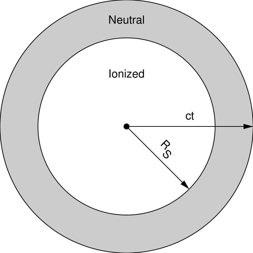
Figure 10: Schematic diagram of early evolution of a Strömgren sphere. The outer circle of radius $ct$ marks the extent (in the absence of absorption) of the ionizing radiation at a time $t$ after the source turns on. The inner circle of radius $R_{S}$ is the ionized Strömgren sphere. The number of photons in the shaded volume is equal to the number of hydrogen atoms in the ionized volume.

With these assumptions, ionizing photons propagate freely to the edge of the ionized region where they are immediately absorbed by the neutral gas. Figure 10 shows the relevant geometry. The photons that would have traveled beyond the Strömgren radius $R_{S}$ (the shaded region) have been absorbed by neutral hydrogen atoms within $R_{S}$. The size of the H II region is determined by a balance between the number of photons in the outer shell and the number of atoms within the ionized sphere:

$${\dot{N}}_{ph}\left(t-{R_{S}\over c}\right)={4\pi R_{S}^{3}n_{H}\over 3}\quad,$$ (A1)

where ${\dot{N}}_{ph}$ is the ionizing photon luminosity and $t$ is the age of the source. This cubic equation can be analytically solved to give

$$R_{S}(t)={3y\over y^{2}+y+1}ct\quad,$$ (A2)

where

$$y=\left({3^{3/2}\over 2}{t\over t_{c}}+\sqrt{{27\over 4}\left(t\over t_{c}\right)^{2}+1}\right)^{2/3}$$ (A3)

and the time $t_{c}$, which roughly marks the end of the relativistic expansion period, is

$$t_{c}=\left(3{\dot{N}}_{ph}\over 4\pi n_{H}c^{3}\right)^{1/2}=1.2\times 10^{7}\,\hbox{yr}\,\left({\dot{N}}_{ph}\over 10^{57}\,\hbox{s}^{-1}\right)^{1/2}\,\left(1+z_{Q}\over 7\right)^{-3/2}\,\left({n_{\rm HI}\over n_{\rm H}}{\Omega_{b}h^{2}\over 0.0196}\right)^{-1/2}\quad,$$ (A4)

where $z_{Q}$ is the quasar redshift. Here we have explicitly included the dependence on the neutral fraction $n_{\rm HI}/n_{\rm H}$ and the cosmological parameters.

Figure 11: Size versus time for early Strömgren sphere expansion. The time is scaled by $t_{c}$, the duration of relativistic expansion (see text for details) and the radius by $R_{c}=ct_{c}$. The dashed line is $R=ct$. At late times the expansion is $R\sim t^{1/3}$.

The expansion law in Eqn. (A2) is shown in Figure 11. After an initial period where the ionization front moves out at nearly the speed of light, the expansion slows and approaches the standard $t^{1/3}$ law (Madau & Rees 2000, Cen & Haiman 2000).

This is not, however, the expansion law that is observed via absorption along the line-of-sight. When we observe Ly$\,\alpha$ absorption from the neutral gas just beyond the edge of the H II region, the Ly$\,\alpha$ photons being detected were emitted only a short time after the first ionizing photons. Specifically, if the Ly$\,\alpha$ photons cross the Strömgren boundary at a radius $R_{S}$, they were emitted when the age of the quasar was only $t^{\prime}=t-R_{S}/c$ (which is the time for light to cross the outer, shaded shell in Fig. 10). The observed Strömgren evolution, as inferred from absorption, is not $R_{S}(t)$ versus $t$ but rather $R_{S}(t)$ versus $t^{\prime}$. With some algebraic manipulation of the analytical expressions for $R_{S}$ and $t^{\prime}$, we can express $R_{S}$ directly in terms of the observed (apparent) time $t^{\prime}$ as

$$R_{S}=R_{c}\left(t^{\prime}\over t_{c}\right)^{1/3}\quad,$$ (A5)

where $R_{c}=ct_{c}$.

This is a surprising result (at least, it surprised us!) The expansion law for the observed radius is exactly the same as the expansion law derived if one completely ignores light-travel time effects (eq. 6). In the frame of the quasar the ionization front’s expansion velocity is limited by the speed of light, but for the observer there is an initial period of superluminal expansion. The speed of light drops out of the solution along the line-of-sight because the delay required to allow light to travel from the source to the edge of the H II region is exactly compensated by the speedup that results from that edge being closer to the observer, allowing light originating there to reach the observer sooner than light from the quasar core.

Note that the size of the observed H II region in Eqn. (A5) may be larger than the ionized region that exists at the end of the quasar’s lifetime. For example, suppose a quasar shines for a period $t_{c}$ and then shuts down. According to Eqn. (A2), at $t_{c}$ the radius of the H II region is $0.7\,R_{c}$. But the observer measures a radius $R_{c}$ (eq. A5). What is happening in this case is that the H II region continues to expand after the quasar shuts off until it reaches a maximum size $R_{c}$ at $t=2t_{c}$. At that point the inner sphere in Figure 10 is completely empty of ionizing photons and so the expansion stops. The observer is detecting Ly$\,\alpha$ photons that were emitted just at the end of the quasar’s lifetime, but by the time those photons cross the ionization front it has expanded to its maximum size.

Our conclusion is that when all the light travel time effects are taken into account, Eqn. (A5) is the correct formula for computing the age of the quasar given the luminosity. Ages determined using that formula are, in fact, the age of the quasar at the time it emitted the photons being detected, and so such ages are direct measurements of the minimum quasar lifetime even during the superluminal expansion phase.

References

- Barkana (2002) Barkana, R. 2002, New Astronomy, 7, 337
- Becker et al. (2001) Becker, R. H. et al. 2001, AJ, 122, 2850
- Brotherton et al. (2001) Brotherton, M. S., Tran, H. D., Becker, R. H., Gregg, M. D., Laurent-Muehleisen, S. A., & White, R. L. 2001, ApJ, 546, 775
- Cen & Haiman (2000) Cen, R. & Haiman, Z. 2000, ApJ, 542, L75
- Cen (2003) Cen, R. 2003, ApJ, submitted (astro-ph/0210473)
- Coifman & Donoho (1995) Coifman, R.R., & Donoho, D.L. 1995, in Wavelets and Statistics, Lecture Notes in Statistics, eds. A. Antoniadis & G. Oppenheim (New-York: Springer-Verlag), p. 125
- Comerford, Haiman, & Schaye (2002) Comerford, J. M., Haiman, Z., & Schaye, J. 2002, ApJ, 580, 63
- Donoho & Johnstone (1994) Donoho, D. L., & Johnstone, I. M. 1994, Biometrika, 81, 425
- Djorgovski, Castro, Stern, & Mahabal (2001) Djorgovski, S. G., Castro, S., Stern, D., & Mahabal, A. A. 2001, ApJ, 560, L5
- Elvis et al. (1994) Elvis, M. et al. 1994, ApJS, 95, 1
- Fan et al. (2001) Fan, X. et al. 2001, AJ, 122, 2833
- Fan et al. (2002) Fan, X., Narayanan, V. K., Strauss, M. A., White, R. L., Becker, R. H., Pentericci, L., & Rix, H. 2002, AJ, 123, 1247
- Fan et al. (2003) Fan, X., et al. 2003, AJ, in press (astro-ph/0301135)
- Fan et al. (2003b) Fan, X., et al. 2003, in preparation
- Francis et al. (1991) Francis, P. J., Hewett, P. C., Foltz, C. B., Chaffee, F. H., Weymann, R. J., & Morris, S. L. 1991, ApJ, 373, 465
- Gnedin & Ostriker (1997) Gnedin, N. Y. & Ostriker, J. P. 1997, ApJ, 486, 581
- Gunn & Peterson (1965) Gunn, J. E. & Peterson, B. A. 1965, ApJ, 142, 1633
- Haar (1910) Haar, A. 1910, Math. Ann., 69, 331
- Haiman (2002) Haiman, Z. 2002, ApJ, 576, L1
- Haiman & Cen (2002) Haiman, Z. & Cen, R. 2002, ApJ, 578, 702
- Haiman & Loeb (2001) Haiman, Z. & Loeb, A. 2001, ApJ, 552, 459
- Hu et al. (2002) Hu, E. M., Cowie, L. L., McMahon, R. G., Capak, P., Iwamuro, F., Kneib, J.-P., Maihara, T., & Motohara, K. 2002, ApJ, 568, L75; Erratum, ApJ, 576, L99
- Kodaira et al. (2003) Kodaira, K., et al. 2003, PASJ, submitted (astro-ph/0301096)
- Kogut et al. (2003) Kogut, A., Spergel, D. N., Barnes, C., Bennett, C. L., Halpern, M., Hinshaw, G., Jarosik, N., Limon, M., Meyer, S. S., Page, L., Tucker, G. S., Wollack, E., & Wright, E. L. 2003, ApJ, submitted (astro-ph/0302213)
- Mackey, Bromm, & Hernquist (2003) Mackey, J., Bromm, V., & Hernquist, L. 2003, ApJ, 586, 1
- Madau & Rees (2000) Madau, P. & Rees, M. J. 2000, ApJ, 542, L69
- Malhotra & Rhoads (2002) Malhotra, S. & Rhoads, J. E. 2002, ApJ, 565, L71
- Miralda-Escudé (1998) Miralda-Escudé, J. 1998, ApJ, 501, 15
- Ouchi et al. (2003) Ouchi, M. et al. 2003, ApJ, 582, 60
- Pentericci et al. (2002) Pentericci, L. et al. 2002, AJ, 123, 2151
- Shapley, Steidel, Adelberger, & Pettini (2002) Shapley, A. E., Steidel, C. C., Adelberger, K. L., & Pettini, M. 2002, American Astronomical Society Meeting, 201, 32.05
- Sheinis et al. (2002) Sheinis, A. I., Bolte, M., Epps, H. W., Kibrick, R. I., Miller, J. S., Radovan, M. V., Bigelow, B. C., & Sutin, B. M. 2002, PASP, 114, 851
- Songaila, Hu, Cowie, & McMahon (1999) Songaila, A., Hu, E. M., Cowie, L. L., & McMahon, R. G. 1999, ApJ, 525, L5
- Songaila & Cowie (2002) Songaila, A. & Cowie, L. L. 2002, AJ, 123, 2183
- Telfer, Zheng, Kriss, & Davidsen (2002) Telfer, R. C., Zheng, W., Kriss, G. A., & Davidsen, A. F. 2002, ApJ, 565, 773
- van Leer, B. (1977) van Leer, B. 1977, J. Comp. Phys., 23, 276.
- Venkatesan, Tumlinson, & Shull (2003) Venkatesan, A., Tumlinson, J., & Shull, J. M. 2003, ApJ, 584, 621
- Wheaton et al. (1995) Wheaton, W. A., Dunklee, A. L., Jacobsen, A. S., Ling, J. C., Mahoney, W. A., & Radocinski, R. G. 1995, ApJ, 438, 322
- Willott, McLure & Jarvis (2002) Willott, C. J., McLure, R. J., & Jarvis, M. J. 2003, ApJ, in press (astro-ph/0303062)
- Wyithe & Loeb (2002) Wyithe, J. S. B. & Loeb, A. 2002, ApJ, 577, 57
- Wyithe & Loeb (2003) Wyithe, J. S. B. & Loeb, A. 2003, ApJ, 586, 693