Long-term X-ray variability of Circinus X-1

Abstract

We present an analysis of long term X-ray monitoring observations of Circinus X-1 (Cir X-1) made with four different instruments: Vela 5B, Ariel V ASM, Ginga ASM, and RXTE ASM, over the course of more than 30 years. We use Lomb-Scargle periodograms to search for the $\sim$16.5 day orbital period of Cir X-1 in each of these data sets and from this derive a new orbital ephemeris based solely on X-ray measurements, which we compare to the previous ephemerides obtained from radio observations. We also use the Phase Dispersion Minimization (PDM) technique, as well as FFT analysis, to verify the periods obtained from periodograms. We obtain dynamic periodograms (both Lomb-Scargle and PDM) of Cir X-1 during the RXTE era, showing the period evolution of Cir X-1, and also displaying some unexplained discrete jumps in the location of the peak power.

1 Introduction

Cir X-1 was discovered in 1971 (Margon, Lampton, Bowyer, & Cruddace, 1971) though it was most likely detected as early as 1965 in a survey conducted by Friedman and collaborators at NRL (Friedman, Byram, & Chubb, 1967). Observations made with the Uhuru satellite from 1971 to 1973 (Jones, Giacconi, Forman, & Tananbaum, 1974) suggested that it was a binary source with a period longer than 15 days. Observations by Ariel V over 1975-76 resulted in the determination of a 16.6 day period (Kaluzienski, Holt, Boldt, & Serlemitsos, 1976). A binary model was proposed in which the high state occurs near the periastron of a highly elliptical orbit (Clark, Parkinson, & Caswell, 1975). Cir X-1 was initially classified as a BHC due to its temporal and spectral similarities to Cyg X-1: millisecond variability (Toor, 1977), flickering in the hard state and very soft energy spectrum in the high state. It has also been found to display a high energy ($>$ 20keV) power law tail which is considered a signature of BHCs (Iaria et al., 2001). The observation by EXOSAT of Type I X-ray bursts (Tennant, Fabian, & Shafer, 1986) in 1985, however, led to the classification of Cir X-1 as a neutron star. It is normally classified as a Low Mass X-ray Binary (LMXB), although doubts still remain about the spectral type of the companion (Moneti, 1992), with some authors proposing an intermediate, 3-5 $M_{\odot}$ companion (Johnston, Wu, Fender, & Cullen, 2001). The orbital period of Cir X-1 is longer than any other LMXB (Lewin, van Paradijs, & van den Heuvel, 1995). The recent discovery of P-Cygni profiles (Brandt & Schulz, 2000) implies the presence of strong winds, which those authors interpret to be coming from an X-ray heated accretion disk, implying that Cir X-1 is probably being viewed edge-on. Radio observations show that Cir X-1 displays relativistic jet-like emission (Fender et al., 1998) leading to its classification as a microquasar. These jet-like features appear to trail back towards SNR G321.9-0.3 (Fender et al., 1998; Tauris et al., 1999) causing some to speculate that Cir X-1 is the remains of a young (age $\sim$20,000–100,000 years), asymmetric supernova. Recent HST observations (Mignani, De Luca, Caraveo, & Mirabel, 2002), however, rule out any association between Cir X-1 and SNR G321.9-0.3, thereby eliminating the age constraint imposed by such an association and raising the possibility that Cir X-1 could be a much older system.

In this paper, we look at archival observations of Cir X-1 made by Vela 5B, Ariel V ASM, Ginga ASM, and RXTE ASM. The data span over 30 years (from 1969 May to 2002 September) and therefore allow us to test for small changes in the orbital period. We first use periodograms to search for the orbital period in the four different sets of data. From these observations we derive a new orbital ephemeris of Cir X-1, based solely on these X-ray observations (all previous ephemerides were based on radio observations). We then look at dynamic periodograms of the more than 6.5 years of RXTE ASM data. We show that there is a clear coherent periodicity in the flux at the orbital period. Furthermore, we show that this modulation disappears for an extended period of time, during which a separate modulation at $\sim$40 days is detected. This new peak in the periodogram lasts for almost one year, after which the fundamental 16.5 day peak returns (and the 40 day peak disappears).

2 Observations

We used a series of observations taken by four different instruments over the course of the last $\sim$33 years. We chose those instruments which had an ASM and therefore allowed us to study the long-term behavior of the source. Figure 1 shows the composite light curve obtained by incorporating all the observations by the different instruments into one single plot. All the data have been normalized to the Crab. Included in this plot are the EXOSAT observations which displayed the Type I X-ray bursts to illustrate what the flux level of the source was at the time, though in this paper we do not analyze the EXOSAT data. Figure 2 shows the light curves obtained by the four ASM instruments, individually plotted for greater clarity. In the short paragraphs that follow I briefly describe the four instruments for which data was analyzed in this paper.

2.1 Vela 5B

The Vela 5B satellite (Conner, Evans, & Belian, 1969) was placed in orbit on 1969 May 23 and operated until 1979 June 19, although telemetry tracking was poor after mid-1976. The X-ray detector covered the celestial sphere twice per orbit and had an effective area of 26 cm², with an energy range of 3-12 keV. In our analysis we use 485 observations of Cir X-1 made between MJD 40368 and MJD 42692.

2.2 Ariel V

Ariel V was launched on 1974 October 15 and operated until 1980 March 14. The All Sky Monitor (ASM) experiment (Holt, 1976) consisted of two small X-ray pinhole cameras with an effective area of $\sim$1 cm² and an energy range of 3-6 keV. In this paper we look at 1173 observations of Cir X-1 made between MJD 42345 and MJD 42692.

2.3 Ginga ASM

The Ginga observatory was launched on 1987 February 5 and reentered the Earth’s atmosphere on 1991 November 1. The ASM instrument (Tsunemi et al., 1989) consisted of two proportional counters operating in the 1–20 keV energy range, covered by six different collimators, each with a field of view of roughly 1${}^{\circ}\times$45^∘ (FWHM) and an effective area of $\sim$70 cm² (for a total effective area of $\sim$420 cm²). For more details of the Ginga ASM see Tsunemi et al. (1989). In this paper, we analyze 300 observations of Cir X-1 taken between the dates of MJD 46855 and MJD 48532.

2.4 RXTE ASM

The Rossi X-ray Timing Explorer (RXTE) (Bradt, Rothschild, & Swank, 1993), was launched on 1995 December 30. The ASM instrument (Levine et al., 1996) consists of 3 Scanning Shadow Cameras (SSCs) with a total effective area of 90 cm² and a sensitivity to 1.5–10 keV X-rays in three energy channels (roughly corresponding to 1.5–3, 3–5, and 5–12 keV). Both individual “dwell” by “dwell” (where a “dwell” refers to a 90 s observation) and one-day average measurements are made available by the ASM/RXTE team via their website. The data used in this paper spanned the dates MJD 50088 (6 January 1996) through MJD 52536 (19 September 2002) and consisted of 1972 daily-averaged measurements.

3 Data Analysis and Results

We computed the Lomb-Scargle periodograms (Scargle, 1982) of the four different data sets. These are shown in Figure 3. A fiducial period of 16.6 days is shown on each plot with dashed lines, for comparison between the different epochs. We found peaks in our periodograms for Vela 5B data (16.69 $\pm$ 0.015 days), Ariel V (16.66 $\pm$ 0.01 days), Ginga ASM (16.577 $\pm$ 0.001 days), and RXTE ASM (16.5427 $\pm$ 0.0001 days). We computed the uncertainty on the period through Monte Carlo simulations of 1000 light curves, assuming the errors on the counting rate have a gaussian distribution. After computing the periodograms of the 1000 light curves generated, we took the mean and standard deviation of the peak frequency.

We also used the Phase Dispersion Minimization (PDM) technique (Stellingwerf, 1978) and compared the values obtained from this method with the periods obtained from the Lomb-Scargle periodograms. Our results are shown in Figure 4: Vela 5B data (16.67 $\pm$ 0.01 days), Ariel V (16.644 $\pm$ 0.001 days), Ginga ASM (16.565 $\pm$ 0.004 days), and RXTE ASM (16.5421 $\pm$ 0.0001 days).

Finally, Fourier analysis was performed on each of the archival data sets to search for orbital periodicities. A detailed review of Fourier analysis techniques in X-ray timing is given by van der Klis (1989). We used a bin time of 7 days for the Fast Fourier Transform (FFT). This gives a Nyquist frequency of $8.267\times 10^{-7}$, or a minimum period of 14.0 days. The analysis was performed by oversampling the FFT. This process creates an FFT with finer detail than a non-oversampled FFT. However, not all of the bins are independent. This method allows one to estimate the frequency of the maximum power in a power density spectrum (PDS) to better accuracy. In Middleditch (1976) it is shown that if the peak power in the signal occurs in frequency bin $k$ (where $k$ need not be an integer), then the best estimate of the signal frequency is given by

$$\hat{\nu}_{0}=\nu_{k}+\frac{3}{4\pi^{2}\epsilon T}\left(\frac{\bar{P}_{k+\epsilon}-\bar{P}_{k-\epsilon}}{\bar{P}_{k}}\right)$$ (1)

where $\bar{P}$ is normalized power, $T$ is the length of the time series, and $n=1/\epsilon$ is the oversampling factor, for this analysis we used $n=8$. The uncertainty on the frequency determination (Middleditch, 1976) is given by

$$\sigma_{\hat{\nu}_{0}}\approx\frac{1}{2\pi T}\sqrt{\frac{6}{P_{k}}}$$ (2)

The Vela, Ariel and Ginga data sets were each FFT’d as a single data set. The RXTE ASM data set, however, was split into two separate data sets. The first data set spans the dates MJD 50088 through 50829, while the second data set covers the dates from MJD 51575 to MJD 52536. The reason for splitting up the observations is that there is a span of almost two years during which the orbital modulation is not clearly detectable. Starting at around MJD 50830, the period (and power) of the peak intensity in the FFT starts to rapidly decrease until it becomes undetectable. While it reappears soon after MJD 51200, there are other unexplained phenomena in the spectra which prevent a good measurement of the period. We describe this in more detail in section 3.2 of the paper. It is only after MJD 51575 that the orbital modulation once again becomes unambiguously detectable. Table 1 shows the details and results of the FFT analysis, which are also plotted in Figure 5).

Experiment	Start MJD	Stop MJD	Period (days)	error
Vela	40367	42687	16.677	$\pm 0.028$
Ariel	42345	44306	16.664	$\pm 0.029$
Ginga	46855	48531	16.551	$\pm 0.028$
RXTE ASM set 1	50088	50829	16.528	$\pm 0.063$
RXTE ASM set 2	51575	52536	16.502	$\pm 0.019$

Table 1: Period searching results from FFT analysis.

We also used epoch folding techniques to determine the period, but our results were inconclusive. This was most likely due to the changing shape of the pulse profile (see for example Figure 7 for the change in pulse profile in the RXTE era).

3.1 Orbital Ephemerides

Several ephemerides have been published for Cir X-1 over the years. Figure 5 shows some of those most often cited in the literature. Nicolson (1980) published an ephemeris based on radio flares that took place between 1976-1980. This ephemeris gave the following equation for the onset of the Nth onset of flares (phase 0):

$\mathrm{MJD_{N}=43,076.26+N(16.588-1.66\times 10^{-4}N)}$, giving a Ṗ$=-2.00\times 10^{-5}$ (labelled Nicolson 1980 in Figure 5). In the same IAUC, Nicolson reports that using the mean X-ray/radio period of 16.594 days derived for 1976-1977 he obtains the following ephemeris:

$\mathrm{MJD_{N}=43,076.26+N(16.594-2.5\times 10^{-4}N)}$, giving a Ṗ$=-3.01\times 10^{-5}$ (labelled Nicolson 1980 b in Figure 5)

A more recent ephemeris, also calculated by Nicolson, though reported by Stewart et al. (1991), was based on the onset times of radio flares observed between 1978 and 1988. This gives the following time for phase 0:

$\mathrm{MJD_{N}=43,076.37+N(16.5768-3.53\times 10^{-5}N)}$, which yields a Ṗ$=-4.26\times 10^{-6}$ (labelled Stewart 1991 in Figure 5).

Figure 5 also shows the different data points obtained by applying three different techniques to the four separate data sets. The individual Lomb-Scargle periodograms for each instrument are shown Figure 3. The PDM periodograms for each data set are shown in Figure 4. We also include in Figure 5 the points obtained by using an over sampled FFT (labelled ’Period by FFT’).

We use all the measurements obtained from the various data sets and period-finding techniques to determine a best fit. We fit the period to the function:

$\mathrm{P=P_{0}+}$Ṗ$\mathrm{(T-T_{0})}$ where we use $\mathrm{T_{0}=43,076.37}$.

Our best fit parameters are:

$\mathrm{P_{0}=16.6534\pm 5.6\times 10^{-3}}$ and Ṗ$\mathrm{=-1.6261\times 10^{-5}\pm 1.109\times 10^{-6}}$. The function of best fit is also plotted in Figure 5. This Ṗ gives us a characteristic time scale of P/2Ṗ $\sim$1400 years, which is around a factor of $\sim$4 shorter than that obtained from the previous ephemeris (Stewart 1991).

We suppose that the ephemeris is quadratic (i.e. constant Ṗ) and therefore follows the equation (for small Ṗ):

$\mathrm{MJD_{N}=MJD_{0}+P_{0}N+\frac{1}{2}P_{0}}$Ṗ$\mathrm{N^{2}}$ where N is the cycle number and $\mathrm{MJD_{N}}$ is the Nth occurrence of phase 0. We use the same $\mathrm{MJD_{0}}$ as the previous ephemeris, which combined with the values of $\mathrm{P_{0}}$ and Ṗ obtained from our fit give us our new ephemeris:

$\mathrm{MJD_{0}=43,076.37+N(16.6534-1.354\times 10^{-4}N)}$

3.2 Dynamic periodograms of the RXTE ASM data

Using the RXTE ASM daily averaged data, we performed “dynamic” periodograms by selecting segments of data of length $\sim$200 days and then stepping through the entire data set in increments of 20 days. Each periodogram was taken in the frequency range between 0.02 and 0.2 d^-1 (5 to 50 day period). Although we are oversampling our data in this way and are therefore not producing statistically independent periodograms, this technique nevertheless allows us to observe long-term trends in the time-frequency space which would otherwise not be so clearly visible. We tried several different values for the length of our periodogram, as well as for the step. While these parameters changed the resolution of the figure, the overall features and their time scales remained the same.

The left side of Figure 6 shows a dynamic Lomb-Scargle periodogram, while the plot on the right in the same figure shows a dynamic PDM periodogram. Both plots share many of the same features: the $\sim$16.5 day orbital period is clearly visible in both, along with some harmonics (at 1/2 and 1/3 the orbital period). The PDM dynamic periodogram also shows several sub-harmonics (at 2 and 3 times the orbital period) which are picked out naturally by this period searching technique (Stellingwerf, 1978). A key feature of both plots is the suppression of the 16.5 day peak starting at $\sim$MJD 50830 and lasting for around 270 days, until $\sim$MJD 51100. During this time, the most significant peak in both periodograms is centered at $\sim$40 days.

To make sure that this feature is not an artifact of our periodogram technique, we look at its manifestation in the time domain. We split up the RXTE ASM data into ten separate segments, each roughly of $\sim$250 days in length. Figure 7 shows the different segments of data have folded at the “orbital” period of 16.54 days. The profiles show that in the first several segments of data, the light curve is clearly modulated at the orbital period. However, when we get to the fourth segment (MJD 50839–51081), there is no sign of the modulation. Furthermore, if we take the fourth segment of data and fold it at 40 days, instead of the 16.54, then we see a clear modulation. Figure 8 shows this segment of data folded at 40 days. The inset plot shows the Lomb-Scargle periodogram for the same data, with a clear peak at 40 days (and no detectable peak at $\sim$16.5 days). To further check these results, we took the 10 individual light curves shown in Figure 7 and folded them at a period of 40 days. As expected, only the fourth segment shows a significant modulation at this period, and none of the other nine show this modulation.

The dynamic periodogram also shows an important peak at around 22 days. This peak is present for $\sim$200 days before the 16.5 day peak is suppressed and right before the 40 day peak appears. When the 16.5 day orbital signal finally returns, it starts off at a period slightly shorter than 16.5 days and takes almost 100 days to ramp back up to its previous 16.5 day peak. Finally, there is another feature common to both dynamic periodograms. At around MJD 51410, the 16.5 signal splits into two separate signals, one slightly longer period ($\sim$18.4 days) and one slightly shorter ($\sim$15.9 days). This split lasts for $\sim$165 days, until both signals finally converge back into one at around MJD 51575. This last feature roughly coincides with the point in the light curve where the overall flux of the source begins its steady decline (see Figure 2). After several years in a high flux state, where its baseline flux was greater than 1 Crab, Cir X-1 has begun a steep decline in flux, towards a lower intensity state; a decline which is still in progress.

4 Discussion

Cir X-1 has been extensively monitored now for over 30 years, though there have been long gaps in the observations, as can be seen from Figure 1. The first thing to note about the long-term light curve shown in Figure 1 is the large variation in the source intensity. Ignoring the large variability within the 16.6 day orbit (itself very significant), we see that the overall flux level of the source has gone from about 0.4 Crab at the beginning of the Vela 5B era, down to almost zero a few years later, then increasing at every epoch since then, until reaching a peak of more than 1 Crab in the RXTE era, only to begin its decline once again at $\sim$MJD 51600, a decline which appears to have levelled off at about 0.4 Crab. Included in Figure 1, besides the data from the four observatories which had an ASM, are the individual pointed observations from EXOSAT. It is interesting to note that the Type I X-ray bursts which led to the classification of Cir X-1 as a neutron star (Tennant, Fabian, & Shafer, 1986) were all detected during one EXOSAT observation taken on 1985 August 12 ($\sim$MJD 46290) at a time when Cir X-1 was much dimmer than it has been ever since. The mean rate at the time of the first Type I burst was $\sim$15 cts s^-1 and at the time of the other two it was $\sim$90 cts s^-1 (see Tennant, Fabian, & Shafer (1986) for more details); this corresponds to $\sim$1–5% of the Crab. This has been offered as an explanation as to why no more bursts have ever been observed. However, it appears that Cir X-1 could soon have a flux similar to its 1984-85 level, making it an interesting potential target for detection of new Type I X-ray bursts.

In this paper we have attempted to derive a long-term ephemeris for Cir X-1 based solely on X-ray observations. Using the results we obtained from Lomb-Scargle periodograms, PDM periodograms, and FFT analyses, we derived a line of best fit which provides, as far as we know, the first ephemeris solely derived from X-ray observations. Although the X-ray emission of Cir X-1 is correlated with the radio observations (Stewart et al., 1991), the peak in X-ray emission sometimes precedes and sometimes follows the onset of the radio flares (Shirey, 1998). It would be interesting to compare our newly derived X-ray ephemeris with a more recent one obtained from radio observations, unfortunately since the late 1980’s the radio flares from Cir X-1 have been too weak to update the ephemeris (Shirey, 1998).

We obtain a characteristic time scale of P/2Ṗ $\sim$1400 years, raising the possibility that this is a much younger system than was previously believed. We should note, however, that although we detect a fairly large decrease in the orbital period over the course of the more than 30 years of monitoring, we are not able to confirm this relatively rapid decrease in period in the RXTE observations alone, which span more than 6.5 years. As we have noted (and is clearly visible in the dynamic periodograms in Figure 6), the orbital period of Cir X-1 was not always detectable during the RXTE observations. In our FFT analysis we split up the data into two distinct epochs in which the orbital period was believed to be clearly detectable. While two values we obtain show a decrease in the orbital period (as would be indicated by the ephemeris), our result, given the errors, is consistent with a constant period over the entire RXTE era.

Finally, we have found that there is a period of time of approximately 270 days in which the 16.5 day peak in the periodograms is suppressed. During this time, in which the presumed orbital period is not detectable, a new peak in the periodogram is clearly visible at approximately 40 days. The relationship between these two periods is not clear, and the mechanism which might cause this suppression is not understood. The dramatic drop in flux level seen for Cir X-1 starting at around MJD 51500, though occurring about a year later, could be related in some way.

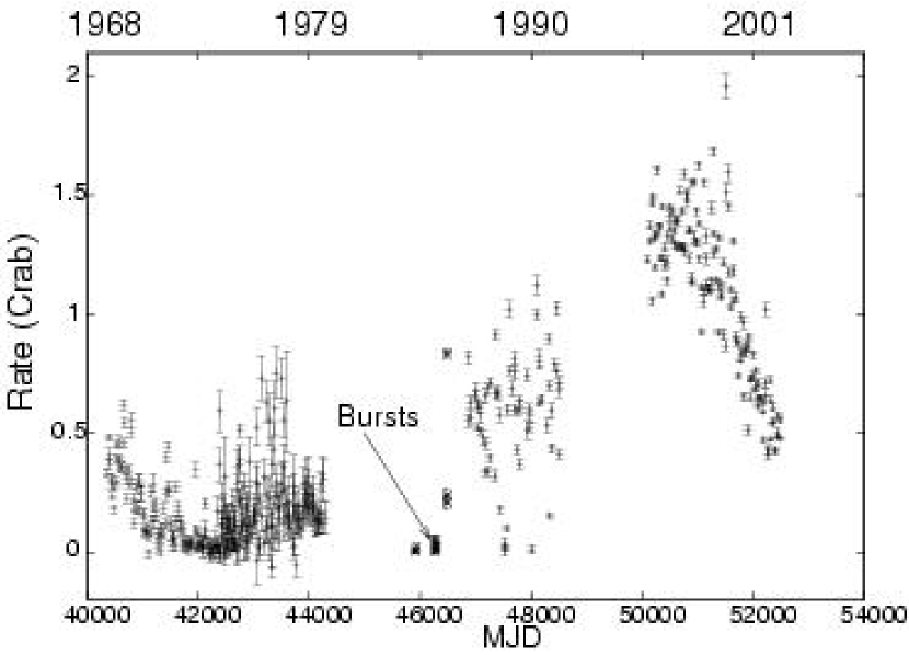
Figure 1: Long-term Light Curve of Cir X-1. Fluxes have been normalized to the Crab. The figure includes data (in chronological order) from Vela 5B, Ariel V ASM, EXOSAT, Ginga ASM, and RXTE ASM. The arrow points to the EXOSAT observations which displayed Type I X-ray bursts.

Figure 2: Individual light curves of Cir X-1 obtained by various instruments. Fluxes have been normalized to the Crab. Top Left – Vela 5B (26 May 1969 - 7 October 1975). Top Right – Ariel V ASM (25 October 1974 - 8 March 1980). Bottom Left – Ginga ASM (1 March 1987 - 2 October 1991). Bottom Right – RXTE ASM (6 January 1996 - 19 September 2002).

Figure 3: Lomb-Scargle periodograms of Cir X-1. The periodograms correspond to the data shown in the light curves in Figure 2. Inset plots show region around the orbital period in greater detail (with the x axis in units of time, for greater clarity). A fiducial period of 16.6 days is shown (with dashed lines) on each plot for comparison between epochs. Top Left – Vela 5B: Peak at 16.69 days. Top Right – Ariel V ASM: Peak at 16.66 days. Bottom Left – Ginga ASM: Peak at 16.57 days. Bottom Right – RXTE ASM: Peak at 16.54 days.

Figure 4: PDM periodograms of Cir X-1. The periodograms correspond to the data shown in the light curves in Figure 2. Inset plots show region around the orbital period in greater detail (with the x axis is in units of time, for greater clarity). A fiducial period of 16.6 days is shown (with dashed lines) on each plot for comparison between epochs. Top Left – Vela 5B: $\Theta_{min}$ at 16.33 days, but a second prominent period is present at $\Theta$=16.67 days. Top Right – Ariel V ASM: $\Theta_{min}$ at 16.64 days. Bottom Left – Ginga ASM: $\Theta_{min}$ at 16.56 days. Bottom Right – RXTE ASM: $\Theta_{min}$ at 16.54 days.

Figure 5: Evolution of the orbital period of Cir X-1. The data points represent the best estimate for the orbital period based on Lomb-Scargle periodograms of the Vela 5B, Ariel V ASM, Ginga ASM, and RXTE ASM data, as well as the PDM periodograms, and the FFT technique (period by FFT).

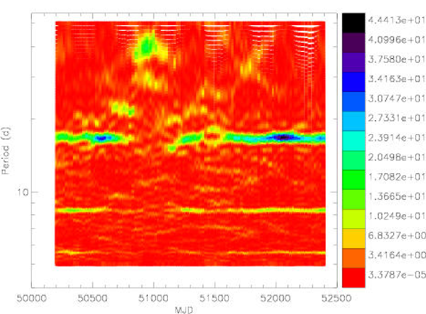
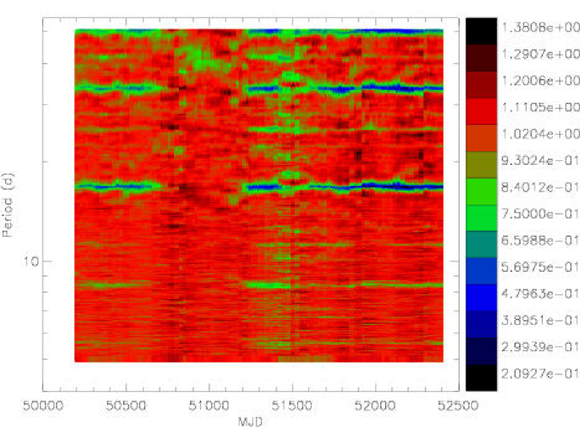
Figure 6: Dynamic Periodogram of RXTE ASM data. A sliding window of length $\sim$200 days was stepped through the entire data set in $\sim$20 day increments. Left – Lomb-Scargle dynamic periodogram. Right – PDM dynamic periodogram.

Figure 7: RXTE ASM data split into 10 segments ($\sim$250 days long each) and folded at the 16.54 orbital period (Phase 0 is at MJD 50082). Segments are ordered from top left (MJD 50088–50337) to bottom right (MJD 52338–52536). Segment 4 (MJD 50839–51081) shows no significant modulation at the 16.54 orbital period.

Figure 8: Main Figure: Segment 4 from Figure 7 (MJD 50839–51081) showing a $\sim$40 day modulation. Inset: Periodogram showing a peak at 40.0 days (and no significant peak at the orbital period 16.5 d).

References

- Bradt, Rothschild, & Swank (1993) Bradt, H. V., Rothschild, R. E., & Swank, J. H. 1993, A&AS, 97, 355
- Brandt & Schulz (2000) Brandt, W. N. & Schulz, N. S. 2000, ApJL, 544, L123
- Clark, Parkinson, & Caswell (1975) Clark, D. H., Parkinson, J. H., & Caswell, J. L. 1975, Nature, 254, 674.
- Conner, Evans, & Belian (1969) Conner, J. P., Evans, W. D., & Belian, R. D. 1969, ApJL, 157, L157
- Fender et al. (1998) Fender, R., Spencer, R., Tzioumis, T., Wu, K., van der Klis, M., van Paradijs, J., & Johnston, H. 1998, ApJL, 506, L121.
- Friedman, Byram, & Chubb (1967) Friedman, H., Byram, E. T., & Chubb, T. A. 1967, Science, 156, 374
- Holt (1976) Holt, S. S. 1976, Ap&SS, 42, 123
- Iaria, Di Salvo, Burderi, & Robba (2001) Iaria, R., Di Salvo, T., Burderi, L., & Robba, N. R. 2001, ApJ, 561, 321.
- Iaria et al. (2001) Iaria, R., Burderi, L., Di Salvo, T., La Barbera, A., & Robba, N. R. 2001, ApJ, 547, 412
- Johnston, Wu, Fender, & Cullen (2001) Johnston, H. M., Wu, K., Fender, R., & Cullen, J. G. 2001, MNRAS, 328, 1193.
- Jones, Giacconi, Forman, & Tananbaum (1974) Jones, C., Giacconi, R., Forman, W., & Tananbaum, H. 1974, ApJL, 191, L71.
- Kaluzienski, Holt, Boldt, & Serlemitsos (1976) Kaluzienski, L. J., Holt, S. S., Boldt, E. A., & Serlemitsos, P. J. 1976, ApJL, 208, L71.
- Levine et al. (1996) Levine, A. M., Bradt, H., Cui, W., Jernigan, J. G., Morgan, E. H., Remillard, R., Shirey, R. E., & Smith, D. A. 1996, ApJL, 469, L33
- Lewin, van Paradijs, & van den Heuvel (1995) Lewin, W. H. G., van Paradijs, J., & van den Heuvel, E. P. J. 1995, Cambridge Astrophysics Series, Cambridge, MA: Cambridge University Press, —c1995, edited by Lewin, Walter H.G.; Van Paradijs, Jan; Van den Heuvel, Edward P.J.,
- Margon, Lampton, Bowyer, & Cruddace (1971) Margon, B., Lampton, M., Bowyer, S., & Cruddace, R. 1971, ApJL, 169, L23.
- Middleditch (1976) Middleditch, J. 1976, Ph.D. Thesis,
- Mignani, De Luca, Caraveo, & Mirabel (2002) Mignani, R. P., De Luca, A., Caraveo, P. A., & Mirabel, I. F. 2002, astro-ph, 0202268
- Moneti (1992) Moneti, A. 1992, A&A, 260, L7.
- Nicolson (1980) Nicolson, M. 1980, IAU Circular, 3449.
- Scargle (1982) Scargle, J. D. 1982, ApJ, 263, 835
- Shirey (1998) Shirey, R. E. 1998, Ph.D. Thesis,
- Stellingwerf (1978) Stellingwerf, R. F. 1978, ApJ, 224, 953
- Stewart et al. (1991) Stewart, R. T., Nelson, G. J., Penninx, W., Kitamoto, S., Miyamoto, S., & Nicolson, G. D. 1991, MNRAS, 253, 212
- Tauris et al. (1999) Tauris, T. M., Fender, R. P., van den Heuvel, E. P. J., Johnston, H. M., & Wu, K. 1999, MNRAS, 310, 1165.
- Tennant, Fabian, & Shafer (1986) Tennant, A. F., Fabian, A. C., & Shafer, R. A. 1986, MNRAS, 219, 871.
- Tennant, Fabian, & Shafer (1986) Tennant, A. F., Fabian, A. C., & Shafer, R. A. 1986, MNRAS, 221, 27P.
- Toor (1977) Toor, A. 1977, ApJL, 215, L57.
- Truemper, Lewin, & Brinkmann (1986) Truemper, J., Lewin, W. H. G., & Brinkmann, W. 1986, S&T, 72, 595
- Tsunemi et al. (1989) Tsunemi, H., Kitamoto, S., Manabe, M., Miyamoto, S., Yamashita, K., & Nakagawa, M. 1989, PASJ, 41, 391
- van der Klis (1989) van der Klis, M. 1989, Fourier Techniques in X-ray Timing, NATO Advanced Study Institute, eds. H. Ogleman, & E. P. J. van den Heuvel, Kluwer Academic Publishers, p. 27-69 (1989).