A ¹³CO and C¹⁸O Survey of the Molecular Gas Around Young Stellar Clusters Within 1 kpc of the Sun

Abstract

As the first step of a multi-wavelength investigation into the relationship between young stellar clusters and their environment we present fully-sampled maps in the J=1–0 lines of ¹³CO and C¹⁸O and the J=2–1 line of C¹⁸O for a selected group of thirty young stellar groups and clusters within 1 kpc of the Sun. This is the first systematic survey of these regions to date. The clusters range in size from several stars to a few hundred stars. Thirty fields ranging in size from $8^{\prime}\times 8^{\prime}$ to $30^{\prime}\times 60^{\prime}$ were mapped with 47^′′ resolution simultaneously in the two J=1–0 lines at the Five College Radio Astronomy Observatory. Seventeen sources were mapped over fields ranging in size from $3^{\prime}\times 3^{\prime}$ to $13^{\prime}\times 13^{\prime}$ in the J=2–1 line with 35^′′ resolution at the Submillimeter Telescope Observatory. We compare the cloud properties derived from each of the three tracers in order to better understand systematic uncertainties in determining masses and linewidths. Cloud masses are determined independently using the ¹³CO and C¹⁸O transitions; these masses range from 30 to 4000  M_⊙. Finally, we present a simple morphological classification scheme which may serve as a rough indicator of cloud evolution.

1 Introduction

It is well established that most stars form in clusters. For example, in an analysis of the 2MASS second incremental release catalogue of the Orion A, Orion B, Perseus and Monoceros molecular clouds, Carpenter (2000) found a total of 1200 isolated stars and $\sim$3000 stars in fourteen clusters, six of these clusters with more than 100 members each. Hodapp (1994) performed a K^′-band survey of 165 regions with known molecular outflows, and found that one third of the outflows were located within a cluster of stars. Clustered star formation spans an enormous range in the number of stars from small groups of several stars in the Taurus dark clouds to the largest known young cluster in our galaxy, NGC 3603, containing many thousands of stars and finally to proto-globular clusters containing up to one million stars. A complete understanding of star formation therefore requires a theory which describes the full range of star formation from small groups to globular clusters.

The formation of stars in clusters is thought to occur over a $\sim$1 Myr time span (e.g. Hillenbrand, 1997; Palla & Stahler, 2000), during which the material to form stars is continually drawn from a reservoir of molecular gas. It is from this reservoir, through a process not fully understood, that fragments condense out of the gas and collapse to form stars. It is therefore likely that the rate of star formation and the number of stars which ultimately form depend on the properties of the molecular reservoir. Previous studies have observed a clear difference between the molecular gas in regions containing small groups of stars, such as Taurus, and regions containing large clusters, such as Orion (Jijina et al., 1999; Onishi et al., 1996; Lada et al., 1991; Lada, 1992; Carpenter et al., 1990, 1995; Tieftrunk et al., 1998). A systematic study of the molecular gas in clusters spanning a range in the number and density of constituent stars can probe in detail how the properties of the parental cluster-forming gas dictates the properties of the forming clusters.

Such a systematic survey could also provide a better picture of the evolution of the cluster-forming molecular gas. The young stars are thought to dissipate the parental cluster-forming gas through winds and radiation, resulting in the termination of ongoing star formation; however, the timescale and exact mechanism of the dissipation remains poorly understood. The process of gas dissipation has been studied in the vicinity of Herbig Ae/Be stars by Fuente et al. (1998a, 2002, hereafter FMBRP), most of which are members of clusters. While these observations provide insight into the mechanism and timescale for the dissipation of gas around individual stars, the dissipation of the extended cluster-forming gas remains to be studied in detail.

We have therefore begun a program of multi-wavelength observations which, when combined with existing infrared and optical data, will yield detailed information about both the stars and their surrounding gas in a large sample of young stellar groups and clusters within 1 kpc of the sun. The final data set will include sensitive ground based wide-field optical and near-infrared imaging and spectroscopy, millimeter spectral-line and continuum maps and mid-infrared observations obtained with the Space Infrared Telescope Facility (SIRTF). Once complete, it will be made available to the community via a web-based database, providing an invaluable resource for future star-formation studies.

In this paper we present our ¹³CO and C¹⁸O molecular line data. C¹⁸O is an excellent tracer of the column density in the warm, dense gas typical of cluster forming regions (Goldsmith, Bergin, & Lis, 1997). Although the freeze out of C¹⁸O has been observed in cold, dark clouds (Bergin et al., 2002), this should only affect small pockets of cold, dense gas within each cluster, such as gravitationally unstable fragments of gas undergoing collapse. The overall structure of the warm gas pervading the cluster is expected to be well traced by C¹⁸O. In addition to tracing the structure of the molecular gas, the C¹⁸O lineshapes and velocities are good tracers of the gas kinematics and are relatively unaffected by optical depth effects. Although emission from the more abundant ¹³CO can be optically thick toward the cluster center, the ¹³CO emission can be traced further into the outer, more tenuous regions of the cluster where C¹⁸O is too weak to be mapped efficiently. These data therefore enable us to characterise the cluster-forming molecular gas from the regions of peak density toward the centers of each cluster out to the non-star-forming gas of the surrounding molecular cloud. Here we concentrate on examining general trends in the morphological properties of the cluster gas. Detailed analysis of the gas kinematics in each of the individual sources will be presented in subsequent papers (Ridge et al. in prep.).

Section 2 describes how our sources were selected, section 3 gives details of the observing and data reduction procedures. An “atlas” of the clusters is presented and cluster properties are compared in section 4. Finally we summarise our main conclusions in section 5.

2 The Sample

To provide a rich sample of sources which are relatively nearby and thus can be observed with high angular resolution and sensitivity, we have compiled from the literature a list of all known young stellar clusters within 1 kpc of the Sun (Christopher et al. in prep.). This list contains a remarkable diversity of regions from small groups with several stars to dense clusters containing hundreds of stars. We use the term “cluster” in this paper to refer to both small groups with five or more stars, and large clusters of several hundred stars. Only these large clusters may eventually form bound open clusters after the dissipation of their parental molecular gas, while most of the smaller systems should quickly disperse (Adams & Myers, 2001). Here we present the subset of regions that are easily observable from the north. Clusters in the regions of Orion and Ophiuchus are not included as they are well studied in the literature. A full list of the objects in the survey, their distances, and the co-ordinates we adopted as the map center for each is given in table A ¹³CO and C¹⁸O Survey of the Molecular Gas Around Young Stellar Clusters Within 1 kpc of the Sun. Where available in the literature the number of stars in the cluster is also given, and a brief summary of previous observations of each source is included in appendix A.

The IRAS point source catalogue was searched for objects within 3^′ of each of the map centers. Where no source could be located within this radius, the search radius was increased in 30^′′ increments until at least one IRAS point source was found. Far-infrared (FIR) luminosities were calculated from the 12–100µm IRAS fluxes using the following formula (Casoli et al., 1986):

$$\frac{L_{\rm FIR}}{L_{\odot}}=4.7\times 10^{-6}D^{2}\left(\frac{S_{12}}{0.79}+\frac{S_{25}}{2}+\frac{S_{60}}{3.9}+\frac{S_{100}}{9.9}\right),$$ (1)

where D is the distance in pc and $S_{\lambda}$ is the flux density in Jy. These luminosities are also listed in table A ¹³CO and C¹⁸O Survey of the Molecular Gas Around Young Stellar Clusters Within 1 kpc of the Sun. If more than one IRAS source was found within the search area then the luminosity of the brightest source is listed. We will use the FIR luminosity in this paper as an indicator of the size (mass) of the stellar component of the clusters, but for more evolved clusters, such as IC 348, where most of the stars are optically visible this assumption is not valid.

Figure 1a shows a histogram of the number of sources with distance. The solid line represents the full sample and the dashed line indicates those sources which were observed at both the Five College Radio Astronomy Observatory (FCRAO) and the Submillimeter Telescope Observatory (SMTO). The histograms show the wide range of distances toward our sample regions, which spans a factor of seven from the nearby L 1551 dark cloud to the distant GGD 4 cluster. This translates into a factor of seven in spatial resolution. The biases this may introduce in a comparative analysis of the clusters are mitigated by the range of cluster properties sampled at a given distance, as shown in Figure 1b. Although there is a trend of increasing FIR luminosity with distance, the upper and lower envelope of this trend differ by a factor of one hundred in luminosity. Futhermore, biases due to distance can be eliminated by comparing regions in the same molecular cloud. In particular, we have two or more clusters within the Perseus cloud, NGC 1499 cloud, Monoceros cloud, the Cepheus cloud, and the Cepheus Bubble. By studying clusters within a single cloud or cloud complex, we can undertake comparative studies which are unaffected by variations in spatial resolution, spatial coverage, or sensitivity.

3 Observations and Data Reduction

3.1 FCRAO Observations

Observations in the ¹³CO 1–0 (110.201 GHz) and C¹⁸O 1–0 (109.782 GHz) transitions were carried out during several periods between 2001 December and 2002 November at the FCRAO 14m telescope in New Salem, Massachusetts, mostly during the commissioning stage of the On-the-Fly (OTF) mapping technique. OTF maps of each of the clusters were made using the SEQUOIA 16-element focal plane array and a dual-IF narrow-band digital correlator, enabling maps in ¹³CO and C¹⁸O to be obtained simultaneously. Observations made after 2002 March utilised the upgraded SEQUOIA-2 array with 32 elements. The correlator was used in a mode which provided a total bandwidth of 25 MHz, with 1024 channels yielding an effective velocity resolution of 0.07 km s^-1. For a few objects (see table 2) data was obtained in the 50 MHz bandwidth mode, with a velocity resolution of 0.13 km s^-1. The weather was exceptionally stable during the runs with system temperatures at 110 GHz generally between 200 and 400 K (single sideband).

Maps were obtained by scanning in the RA direction, and an “off” source reference scan, was obtained after every two rows. Off-positions were checked to be free of emission by performing a single position-switched observation with an additional 30^′ offset. Map sizes are given in table 2. A data-transfer rate (DTR) of either 1 or 2 Hz was used, and in some cases the full size maps were built up from several smaller submaps. When a DTR of 2 Hz was used, maps were repeated to increase signal-to-noise. Calibration was by the chopper wheel technique (Kutner & Ulich, 1981), yielding spectra with units of T${}_{{}_{\rm A}}\!\!\!$*. Pointing was checked regularly and found to vary by less than 5^′′ rms.

The OTF technique was implemented at FCRAO in order to compensate for the removal of the dewar rotation system in the summer of 2001. The maps obtained are therefore not evenly sampled and a convolution and regridding algorithm has to be applied to the data in order to obtain spectra on a regularly sampled grid. This process was carried out using software provided by the observatory (Heyer, Narayanan, & Brewer, 2001). Using this software the individual spectra have a linear baseline subtracted, then are convolved onto a regular 25^′′ grid weighted by 1/rms², yielding a Nyquist sampled map, and corrected for the main beam efficiency of the telescope, which is 0.48 at 110 GHz.

After regridding, the individual spectra had an rms sensitivity of $\sim$0.2 K per 25 kHz channel (see table 2), with the OTF technique yielding maps with extremely uniform sensitivity. Additionally, the simultaneous observation of the two lines gives perfect registration between the ¹³CO and C¹⁸O maps.

3.2 SMTO Observations

Observations in the C¹⁸O 2–1 (219.560 GHz) transition were carried out at the Heinrich-Hertz Telescope (HHT) during several periods in the winter and spring of 2001–2002. The receiver was a single channel SIS mixer with a double sideband receiver noise temperature of about 120 K, depending on receiver tuning. The total (single sideband) system noise temperature was between 270 and 500 K depending on weather. The telescope beamsize was 35^′′ at the line frequency. The pointing was checked on well known calibrators or planets, and found to be 2^′′ rms. The main beam efficiency was measured to be 0.78 at the line frequency. However, because of 30% variations in the sideband ratios, the results were scaled to measurements of standard regions such as the Orion KL nebula. Spectra have units of T${}_{{}_{\rm A}}\!\!\!$*.

The data were taken employing OTF mapping. The procedure was first to perform a hot-sky calibration using a chopper wheel, then to map a 2^′ by 2^′ or 2.5^′ by 2.5^′ region. These regions were mapped by scanning in R.A. with a 15^′′ separation between the Declination rows. A reference region either 10^′ or 15^′ lower in R.A. and offset from the center of the map, was used. A measurement on the reference position, which had been previously checked for the presence of emission, was taken before measuring each row. The raw OTF maps were convolved with a Gaussian beam and regridded onto a regular 15^′′ grid in the GILDAS data reduction environment. The final images consist of mosaics of the individual OTF maps. After the regridding process, individual spectra had an rms sensitivity of $\lesssim$0.17 K per 250 kHz (=0.34  km s^-1) channel.

4 Results

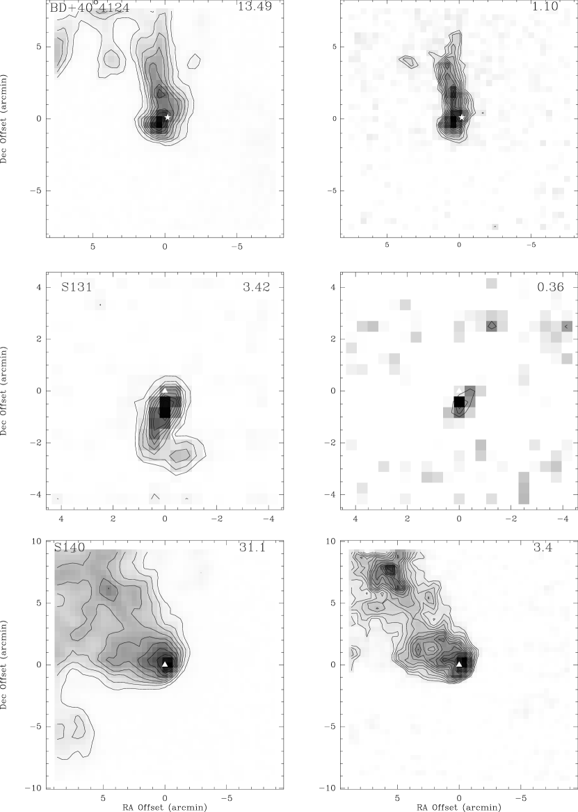
Figure 2: Integrated intensity maps of BD+40^∘4124 (top) and S 131 (middle) and S 140 (bottom), all classified as developmental Class I. The value of the maximum integrated intensity in K  km s^-1 is given in the top right corner of each panel. Left panels show ¹³CO 1–0 integrated emission, with contours at 10% intervals from 10% to 100% of the maximum integrated intensity. Right panels show integrated C¹⁸O 1–0 emission. Base contour is 3$\sigma$, contour interval is 1$\sigma$, except for S 131 where the base contour is at 2$\sigma$ and contour intervals at 0.5$\sigma$. (0,0) positions are as given in table A ¹³CO and C¹⁸O Survey of the Molecular Gas Around Young Stellar Clusters Within 1 kpc of the Sun. Triangles indicate the position of an IRAS or near-infrared (embedded) source and stars indicate the position of an optically visible Herbig Ae/Be star.

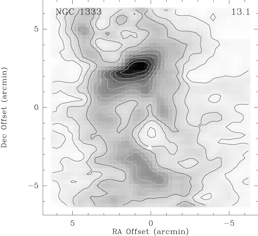
Figure 14: C¹⁸O 2–1 integrated intensity map of NGC 1333. Base contour is at 10%, contour interval is 10% of the maximum integrated intensity, as given in the top right corner of the panel. (0,0) positions are as given in table A ¹³CO and C¹⁸O Survey of the Molecular Gas Around Young Stellar Clusters Within 1 kpc of the Sun. Symbols are as in figure 2.

Integrated intensity maps of the ¹³CO 1–0 and C¹⁸O 1–0 emission are presented in figures 2 through 13. The ¹³CO 1–0 maps have contours at 10% to 100% of the maximum integrated intensity with intervals of 10%, except where indicated otherwise in the caption. The base contour level is $\gg 3\sigma$. The C¹⁸O 1–0 maps have a base contour level of 3$\sigma$, with contours at 1$\sigma$ intervals in most cases. In a few sources different contour levels are used, and are described in the captions. Integrated intensity maps of the C¹⁸O 2–1 emission are presented in figures 14 through 17, with contours at 10% to 100% of the maximum integrated intensity. The value of the maximum integrated intensity in each map is given in the top right corner of the figures for reference. We have indicated the positions of known stellar or protostellar sources in the regions by triangles (embedded sources) or stars (optically-visible sources). The C¹⁸O 1–0 emission was too weak to be detected in only two sources, HD 216629 and VV Ser. This was particularly surprising in HD 216629 where the ¹³CO emission was relatively strong at the peak position.

4.1 Morphology

The clusters show a range of morphologies, from compact, roughly spherical (e.g. CB34), cometary (e.g. S140) to diffuse, extended emission (e.g. VVSer). Based on our examination of the ¹³CO and C¹⁸O maps, we have assigned each source a morphological description, which is listed in table 3. Some of the sources could be placed in more than one category, for instance NGC 7129 shows both a compact core and a cavity. Many of the sources show cores surrounded by more extended envelopes. The emission rarely exhibits circular symmetry; the cores are usually somewhat elongated, and their envelopes are often more elongated than the cores, possibly because the larger envelopes are better resolved. In some cases an elongated core in ¹³CO appears as a chain of multiple cores when observed in C¹⁸O  which is less affected by optical depth (e.g. IC 348). In many cases, multiple peaks are apparent; we have tabulated the number of “significant peaks” (N_peaks) detected in ¹³CO for each region in table 3. We have used the ¹³CO data to identify peaks due to the higher signal to noise in this tracer; however, in several cases, additional peaks are apparent in the C¹⁸O maps due to the lower optical depth in the C¹⁸O lines.

In many of the clusters, the most luminous members have been identified, either through the IRAS point source catalog, or through catalogs of Herbig Ae/Be stars (Testi et al., 1997, 1998). As an indicator of whether the observed ¹³CO peaks contain known sites of recent or ongoing star formation, the distance (d_∗) between the embedded source or star and its nearest ¹³CO peak is shown for each source in table 3. In cases where there are multiple peaks and/or stars, the smallest distance is reported.

The observed structures in the ¹³CO and C¹⁸O maps are most likely a combination of features due to initial conditions in the cloud and interaction with already formed stars. The compact cores, such as GGD 4 and CB 34 are likely to be still close to their initial state, while clouds with cavities such as HD 200775 are breaking apart due to star-cloud interactions. Most of the Herbig Ae/Be type stars in the sample appear to be located in regions which have morphologies consistent with dispersal of their surrounding molecular gas, while the embedded sources appear to be preferentially located in gas which is more centrally condensed. Nineteen of the thirty regions have ¹³CO peaks coincident with or close to a stellar or IRAS position. All but two of these display a centrally condensed morphology (core or core + envelope). We therefore interpret the proximity of the stellar source to the map peak as an indicator of youth of the region. Based on these interpretations we propose a sequence of morphologies, or “developmental classes” as follows:

I

A single significant peak in ¹³CO and C¹⁸O indicative of one dominant molecular core. An extended envelope is commonly detected around the core. An embedded source is found within the 50% contour of the peak C¹⁸O emission, e.g. CB 34. Eleven of the clusters fall into this class, including a subset of five bright-rimmed globules, noted by “BRG” in table 3. The BRGs all show “tails” of extended ¹³CO emission.

II

The ¹³CO and C¹⁸O emission is distributed in multiple peaks and/or elongated filaments, often with an extended envelope. An embedded source falls within the 50% contour of a C¹⁸O peak or filament, e.g. S 171. In some cases with two known associated sources (e.g. NGC 7129), one of the sources is located outside of peaks. Ten sources fall into this class.

III

Known stars fall well outside of ¹³CO and C¹⁸O peaks and filaments, e.g. HD 200775. Typically show diffuse, extended emission, multiple ¹³CO peaks, and multiple or no C¹⁸O peaks. In one region, IC348, two of the three associated sources fall outside the ¹³CO emission. Nine sources fall into Class III.

The classifications are listed in table 3, and figures 2 through 10 are grouped according to classification. Since many of the Class I and III sources show similar FIR luminosities, it is likely that the differing morphologies reflect an evolutionary progression from Class I to Class III driven by the disruption of the gas by the embedded stars. Due to their morphological complexity, Class II sources are more problematic. Many of these regions may be coeval with Class I sources, indicating different initial conditions, while others showing distinct signs of gas dispersion (e.g. NGC 7129) may be in an intermediate evolutionary state between Class I and III.

This scheme differs from the the classification scheme of Fuente et al. (1998a, 2002), although the Fuente et al. sample contains several sources in common with this work. Fuente et al. mapped small regions ($\sim$1 pc) around each of their sources in order to determine the molecular gas distribution close to the Herbig Ae/Be stars, while in contrast, our proposed classification is based on the global morphology of the cluster forming cloud. However, of the six sources common to both Fuente et al. and this work (MWC 297, HD 200775, HD 216629, VV Ser, BD+65^∘1637 and LkH$\alpha$234), both classification schemes place these sources as the most evolved regions of the sample, with one exception, NGC 7129, but this is due to our treatment of the region as a whole, while Fuente et al. considered the two stellar sources separately. We see significant molecular gas emission away from the location of the star, and outside the region covered by Fuente et al. in most cases.

4.2 Masses

The core masses determined from the three isotopomers/transitions are given in table 4. Gas masses were determined from the ¹³CO and C¹⁸O 1–0 transitions using a local thermal equilibrium (LTE) approximation, assuming an excitation temperature of 20 K and the distances given in table A ¹³CO and C¹⁸O Survey of the Molecular Gas Around Young Stellar Clusters Within 1 kpc of the Sun. This method has been found to be accurate to within a factor of 2–4 (Rohlfs & Wilson, 2000) as long as the actual excitation temperature is less than 30 K. Such high excitation temperatures are expected only toward the embedded OB stars that occupy a small fraction of the total cloud area in any of these regions. The C¹⁸O 2–1 masses were determined by calculating the column density of H₂ from the large velocity gradient (LVG) relation:

$$N_{\rm H_{2}}=2.65\times 10^{21}\int T_{\rm MB}(C^{18}O,J=2\rightarrow 1){\rm d}v,$$ (2)

where $v$ has units of  km s^-1, $T_{\rm MB}$ of Kelvins and $N_{\rm H_{2}}$ is given in cm^-2 (Rohlfs & Wilson, 2000). $N_{\rm H_{2}}$ can then be converted to a total gas mass by assuming a distance (as given in table A ¹³CO and C¹⁸O Survey of the Molecular Gas Around Young Stellar Clusters Within 1 kpc of the Sun), the mass of the hydrogen molecule and a helium abundance. For comparison, we have also calculated the LTE mass from the C¹⁸O 1–0 emission for the smaller area covered by the C¹⁸O 2–1 observations (hereafter referred to as the central C¹⁸O mass) and this is given in column 5 of table 4.

We compare the masses derived from each of the three transitions in figure 18, in order to investigate how the choice of tracer and map size will affect our results. Figure 18b shows the central C¹⁸O 2–1 mass plotted against the central C¹⁸O 1–0 mass. The central mass determinations for the two C¹⁸O transitions are very consistent, indicated by the dashed line showing the 1:1 relation. Just two sources, GGD 12-15 and CepC fall significantly from this relation. This plot demonstrates that mass estimates from different transitions using different approximations (LTE vs LVG) lead to equivalent results. Comparison of the central C¹⁸O 2–1 masses, measured with the SMTO, and the total C¹⁸O 1–0 masses in the larger region covered by the FCRAO observations (fig.18c) indicates that a significant fraction of the gas ($\sim$65%) is found in emission that extends outside the smaller C¹⁸O 2–1 maps. Nevertheless, a clear correlation is evident, suggesting that the mass in the extended component grows linearly with the mass in the central region.

The correlation between the envelope mass and the central mass is also apparent in the strong correlation ($\sim 9\sigma$) between the ¹³CO and C¹⁸O 1–0 masses (Figure 18a). However, the ¹³CO masses are approximately a factor of two larger than the masses determined from the C¹⁸O 1–0 emission. This is indicated by the solid line on figure 18a which is a least-squares-fit (LSF) to the data, with a slope of 0.58$\pm$0.05. The ¹³CO traces lower density gas since the abundance is 5 to 10 times higher than C¹⁸O and also because photon trapping allows the ¹³CO to be excited at a lower density than C¹⁸O. In addition, the J=1–0 line is more easily excited than the J=2–1 line because the Einstein A coefficient is about a factor of 8 smaller. Therefore the ¹³CO emission is detectable in more extended regions, where the C¹⁸O emission is too weak to detect, and is likely to be mostly due to gas in the envelope which is too diffuse to detect in the weaker C¹⁸O line. The relationship between the ’central’ (C¹⁸O 2–1) and ’total’ (¹³CO 1–0) masses shows a strong correlation ($\sim 9\sigma$) with small scatter (Figure 18d). This is surprising considering the varied morphologies of the sources and the fact that the physical size of the region mapped varies with distance. The line represents a LSF with a slope of 0.23$\pm$0.02, indicating that the central mass is usually $\sim$ 1/4 of the total mass.

Histograms of the ¹³CO 1–0 masses are presented in figure 19. These show that 2/3 of the clouds are below 1000  M_⊙ when measured with ¹³CO, and that 1/3 of the clouds are below 500  M_⊙. Figure 20a shows the C¹⁸O 1–0 masses as a function of distance. Although there is an apparent trend of higher mass with distance, the upper and lower envelope of this trend differ by more than an order of magnitude. This wide range of masses present at any distance interval will minimise biases due to distance in subsequent comparisons of cloud vs. cluster properties. Finally, the C¹⁸O 1–0 mass is plotted against the FIR luminosity in figure 20b. The correlation here ($\sim 4\sigma$), indicating that more massive cores are forming more luminous (massive) stars, is much stronger than any correlation between either mass or FIR luminosity and distance (both $\lesssim 2\sigma$) and therefore this effect is likely to be real.

4.3 Sizes and Linewidths

The sizes and linewidths of the cores are listed in Table 5. We define core size, R, here as $\sqrt{A/\pi}$ where $A$ is the total area in pc² (i.e. number of pixels $\times$ pixel size in pc) where the integrated intensity is $\geq$1/2 the maximum integrated intensity. All the derived sizes are much larger than the telescope resolution, and smaller than the map size. The average FWHM linewidth in the cores was determined by combining all the spectra in the regions of the maps where emission was detected, and then fitting a Gaussian profile to the resultant average spectrum. In a few cases (e.g. Mon R2, S 140 and Ceph A) this is likely to be affected by strong outflows. Note that for multiply-peaked or filamentary sources the definitions of size we make here may not be appropriate; this definition is most applicable to sources which show some degree of circular symmetry.

We compare the linewidths of the 1–0 and 2–1 transitions in figure 21. The C¹⁸O 2–1 linewidth is closely correlated with the C¹⁸O 1–0 linewidth with a best-fit slope close to one. This is expected given the low optical depth of the C¹⁸O transitions. When the two linewidths do differ, the linewidth given by 2–1 transition is in all but two cases smaller. This is likely an effect of the larger field covered with C¹⁸O 1–0 – the inclusion of a larger region of the cloud should typically broaden the average linewidth due to velocity shifts across each map. In most cases, however, the average linewidths are dominated by the stronger line emission in the centers of each region, resulting in the strong correlation seen in figure 21a. The ¹³CO and C¹⁸O 1–0 linewidths do not show the same degree of correlation (figure 21b), with the ¹³CO linewidths typically being higher. This likely due in part to the higher optical depth in the ¹³CO line.

We also calculate the virial mass, M_V, from the tabulated sizes and linewidths using the form of the virial theorem given in Rohlfs & Wilson (2000):

$$\frac{M_{\rm V}}{M_{\odot}}=250\left(\frac{\Delta v_{1/2}}{km\,s^{-1}}\right)^{2}\left(\frac{R}{pc}\right).$$ (3)

The gas mass derived from the C¹⁸O 1–0 data using the LTE analysis and virial theorem are compared in figure 22. The majority of sources show virial masses between one to two times larger than the C¹⁸O mass. This difference will be reduced by the choice of the virial constant; for clouds with $r^{-2}$ density profiles, the virial masses we have calculated will be a factor of two too large (MacLaren et al., 1988). Furthermore, the virial theorem should only be applicable to centrally condensed morhpologies, and should not apply to the many regions showing extended or diffuse morphologies, or exhibiting multiple peaks. Nevertheless, the observation that most virial masses are within a factor of two of the LTE mass suggests that in most of the clouds, the gravitational energy dominates the kinetic energy, and that most of the clouds are graviationally bound.

Larson (1981) found that molecular clouds exhibit a well defined relationship between cloud size and average linewidth. In figure 24, we display the size-linewidth relation for the C¹⁸O 1–0 transition in our sample of regions. This transition should give the most accurate relation because it is unaffected by optical depth effects like the ¹³CO 1–0, but encloses all of the emission, unlike the C¹⁸O 2–1. We find considerable scatter compared to Larson’s relation; however, we cover only an order of magnitude in core size, much smaller than the three orders of magnitude considered by Larson. The scatter may also be increased due to the method we used to calculate the size of the region, which is primarily applicable to clouds showing a circular symmetry.

Figure 23a shows the average C¹⁸O 2–1 linewidth plotted against FIR luminosity. There is a 3.7$\sigma$ correlation between linewidth and luminosity. This is not due to a correlation with distance, as is indicated in fig. 23b – the significance of the correlation between linewidth and distance is only 1.8$\sigma$.

5 Summary

We have begun a program of multi-wavelength observations which, when combined with existing infrared and optical data will yield detailed information about both the stars and their surrounding gas in a large sample of young stellar clusters within 1 kpc of the sun. Here we presented millimeter spectral line maps of a sample of 30 of these cluster-forming regions in the 1–0 transitions of ¹³CO and C¹⁸O. Smaller regions surrounding 17 of these sources were also mapped in the C¹⁸O 2–1 transition. Based on our ¹³CO 1–0 maps and the location of the stellar or protostellar source we proposed a sequence for the morphology of gas surrounding the clusters. The youngest sources have centrally condensed cores containing an embedded source, while the more evolved sources have extended or diffuse molecular gas. Optically visible Herbig Ae/Be stars associated with these sources are often located in cavities, suggestive that these types of stars can be responsible for the dispersal of molecular gas in cluster-forming regions.

We determined cloud masses independently using the three observed ¹³CO and C¹⁸O transitions, and compared the cloud properties derived from each of the three tracers in order to better understand systematic uncertainties in determining masses and linewidths. We found good consistency between the LTE and LVG methods, and between the masses and linewidths derived from C¹⁸O 1–0 and 2–1. Virial masses were found to be within a factor of two of the LTE mass in most of the regions, suggesting that the gravitational energy dominates the kinetic energy in these regions, and that they are graviationally bound.

Fits images of the integrated emission will be made available for general use via the project website. Our final data set will include sensitive ground based wide-field near-infrared imaging and spectroscopy, millimeter spectral-line and continuum maps and mid-infrared observations obtained with SIRTF. Once complete, it will be made available to the community via a web-based database, providing an invaluable resource for future star-formation studies.

Appendix A Individual Sources

In this section we give a brief summary of previous observations of each of the groups and clusters. For clarity we give a selection of just the most recent references on each source.

A.1 Class I

A.1.1 BD+40^∘4124

The Herbig Be star BD+40^∘4124 is the most massive member of a small group of young emission line stars (Hillenbrand et al., 1995), and a large number of highly embedded stars detected in the infrared by Palla et al. (1995). There is also a small molecular outflow in the region, probably driven by the embedded source V1318S (catalog ) (Palla et al., 1995).

A.1.2 S 131

S 131, also called Ceph OB Cloud 37 is a bright-rimmed cloud associated with an Hii region (Sugitani, Fukui, & Ogura, 1991) and the Galactic open cluster IC 1396 (catalog ). A small cluster was observed in this region by Sugitani et al. (1995), and several H$\alpha$ emission-line stars were detected by Ogura, Sugitani, & Pickles (2002). Interferometric C¹⁸O observations of this region were made by Sugitani et al. (1997).

A.1.3 S 140

The S 140 region is a prototypical cometary globule, photoionised on the south-west side by the B0 star HD 211880 (catalog ). It contains at least three bright infrared sources. A high-velocity molecular outflow was detected in ¹²CO observations by Snell et al. (1984). Previous smaller scale molecular line observations have been made by Minchin, White, & Padman (1993) who determined that the outflow was driven by the source IRS 1.

A.1.4 L 1206

L 1206 is a bright-rimmed globule associated with the Hii region S 145. It has a molecular outflow, discovered in a survey by Sugitani et al. (1989).

A.1.5 Cep A

The Cepheus A region is a molecular cloud containing a very active star forming region indicated by a powerful molecular outflow (Rodríguez, Moran, & Ho, 1980b), more than 25 water masers (Torrelles et al., 1996) and numerous thermal and non-thermal radio sources (Hughes, 2001; Garay et al., 1996).

A.1.6 AFGL 490

AFGL 490 is a relatively isolated infrared source in the Cam OB1 complex (Chini, Henning, & Pfau, 1991). It is a young massive star-forming region, containing a cluster of embedded sources (Hodapp, 1994) and associated with a molecular outflow (Snell et al., 1984), and maser emission (Henkel, Guesten, & Haschick, 1986).

A.1.7 GGD 4

GGD 4 contains a small cluster of young stars (Hodapp, 1994) and the driving source of a molecular outflow (Fukui, 1989).

A.1.8 CB 34

CB34 is a relatively distant large globule containing a small group of infrared sources (Alves & Yun, 1995), at least two high-velocity jets (Khanzadyan et al., 2002) and several millimeter continuum sources thought to be very young protostars (Huard, Weintraub, & Sandell, 2000).

A.1.9 Mon R2

This is an association of B1-B9 stars located in the Mon R2 giant molecular cloud. It is a very active star-forming region, associated with a powerful molecular outflow (Bally & Lada, 1983; Tafalla et al., 1997), a compact Hii region (Wood & Churchwell, 1989), an infrared cluster (Carpenter, 2000), and OH masers (Minier et al., 2001).

A.1.10 GGD 12-15

GGD 12–15 is an active star-forming region embedded in the Monoceros molecular cloud. It is associated with a strong water maser, a cometary compact Hii region (Rodríguez et al., 1978, 1980a; Gomez et al., 1998), several millimeter-continuum sources and a bipolar CO outflow (Little, Heaton, & Dent, 1990).

A.1.11 NGC 2264

The NGC 2264 region in northern Monoceros contains two well studied star formation regions, IRS 1 and IRS 2. Thirty IRAS sources, most classified as Class I protostars (Margulis, Lada, & Young, 1989) are present, as well as $\sim$360 near-infrared sources (Lada, Young, & Greene, 1993). At least nine molecular outflow sources were identified in an unbiased survey by Margulis & Lada (1986).

A.2 Class II

A.2.1 IRAS 20050

The region IRAS 20050 contains an embedded star and an extremely-high-velocity (EHV) molecular jet and multipolar molecular outflow, likely the superposition of outflows from several young stars (Bachiller, Fuente, & Tafalla, 1995).

A.2.2 S 106

The S 106 region contains a bipolar Hii region and an associated molecular cloud. Near-infrared observations by Hodapp & Rayner (1991) revealed a cluster of 160 young stars in this region. A recent much deeper near-infrared survey of the region suggests that the total number of young stars could be much greater ($\sim$ 600) (Oasa et al., 2002). CO observations of this region were made by Schneider et al. (2002).

A.2.3 NGC 7129

NGC 7129 is a reflection nebula in the region of a young cluster, containing three B-type stars (BD+65^∘1638 (catalog ), BD+65^∘1637 (catalog ) and LkH$\alpha$234) and several embedded infrared sources. It is associated with Herbig-Haro objects and several molecular outflows (Font, Mitchell, & Sandell, 2001, and refs. therein). Submillimeter continuum observations by Font et al. (2001) reveal several sources which they interpret as prestellar. FMBRP have made higher-resolution ¹³CO and C¹⁸O 1–0 observations of the molecular gas in a small portion of this region, finding a cavity surrounding BD+65^∘1637, while LkH$\alpha$234 is located at the peak of ¹³CO emission. Molecular line observations of the region were also made by Miskolczi et al. (2001).

A.2.4 S 140-N

The region S 140-N contains a molecular outflow, discovered by Fukui et al. (1986). Davis et al. (1998) made a higher resolution ¹²CO 2–1 map of the outflow and determined that it is powered by the intermediate-luminosity IRAS source 22178+6317 (catalog ). To the east of the molecular outflow source are a sequence of Herbig-Haro objects (HH 251-254 (catalog )) oriented in a northwest-southeast direction indicating a second outflow (Eiroa et al., 1993).

A.2.5 L 1211

L 1211 is a dense core in the Cepheus cloud complex. It contains a very young cluster, detected in millimeter continuum observations by Tafalla et al. (1999), and powers two molecular outflows.

A.2.6 Cep C

The Cepheus C region is an isolated core within the Cepheus OB3 molecular cloud (Sargent, 1977). The region contains a cluster of infrared sources (Hodapp, 1994) and is associated with water maser emission (Wouterloot & Walmsley, 1986) and an outflow (Fukui, 1989).

A.2.7 S 171

S 171 is a bright-rimmed cloud associated with the Cepheus OB4 stellar association, an actively star-forming Hii region, and molecular cloud complex (Yang & Fukui, 1992). The main heating and ionizing source of this region is believed to be the star cluster, Be 59 (catalog ) (Okada et al., 2002). Several H$\alpha$ emission-line stars were detected in this region by Ogura et al. (2002).

A.2.8 NGC 1333

NGC 1333 is a reflection nebula associated with a region of recent, extrememly active star formation in the Perseus molecular cloud. A cluster of about 150 low- to intermediate-mass YSOs have been identified in near-infrared images (Aspin, Sandell, & Russell, 1994). The region also contains about 20 groups of Herbig-Haro objects, some with highly collimated jets (Bally, Devine, & Reipurth, 1996). Rodríguez, Anglada, & Curiel (1999) found a total of 44 sources at centimeter wavelengths, most of which are associated or believed to be associated with young stellar objects in the region.

A.2.9 L 1551

L 1551 is a compact molecular cloud located in the southern part of the Taurus region. It shows abundant signs of ongoing star-formation, and contains the infrared source IRS 5, probably the most well-studied low-mass young stellar object in the galaxy. IRS 5 powers a powerful well-collimated bipolar molecular outflow (e.g. Moriarty-Schieven & Snell, 1988), and is associated with several Herbig-Haro objects. Also in the region are several other overlapping molecular outflows and a number of T-Tauri stars (including the well-known sources HL Tau and XZ Tau).

A.2.10 VY Mon

VY Mon is a highly-reddened Herbig Be star in the Mon OB1 (catalog ) region. It is located 85^′′ south of the reflection nebula IC 446.

A.3 Class III

A.3.1 MWC 297

MWC 297 is an extremely reddened Herbig Be star (Drew et al., 1997) seen in projection against the Hii region S 62 (catalog ), although its relationship to the Hii region is not clear. FMBRP have made higher-resolution ¹³CO and C¹⁸O 1–0 observations of a small region surrounding this source. Their observations show evidence for a cavity surrounding the star, within a more diffuse molecular gas environment.

A.3.2 VV Ser

VV Ser was determined to be a Herbig Ae star by Testi et al. (1998). A small region surrounding this star was mapped in ¹³CO and C¹⁸O 1–0 at higher resolution by FMBRP. They detected very litle molecular gas in the vicinity of this star, and interpreted that it was located in a cavity.

A.3.3 HD 200775

HD 200775 is a B3 star located at the northern edge of an elongated molecular cloud. It is the illuminating star of the well-known reflection nebula NGC 7023 (catalog ) and is associated with a bipolar outflow (Watt et al., 1986) and a cluster of H$\alpha$ emission-line stars (Urban et al., 2001). The region has been previously mapped in ¹³CO 1–0 by Fuente et al. (1998b) and FMBRP. These observations show that the star is located within a biconical cavity, that has probably been excavated by a bipolar outflow. However Fuente et al. (1998b) found no evidence for current high velocity gas within the lobes of the cavity.

A.3.4 L 988-e

The L 988-e cloud contains a cluster of bright infrared sources (Hodapp, 1994) coinciding with the position of a molecular outflow (Clark, 1986).

A.3.5 IC 5146

IC 5146 is a young stellar cluster, associated with a reflection nebula illuminated by the B0 V star BD+46^∘3474 (catalog ). Also embedded in the same cloud is the HAeBe variable BD+46^∘3471 (catalog ) and $\sim$100 H$\alpha$ emission-line stars (Herbig & Dahm, 2002).

A.3.6 HD 216629

HD 216629 is a Be star in the Cepheus cloud with a close companion (Pirzkal, Spillar, & Dyck, 1997) and surrounded by a cluster of infrared sources (Testi et al., 1998). Fuente et al. (1998a, 2002) have made ¹³CO 1–0, C¹⁸O 1–0 and CO 2–1 observations of a 1 pc region surrounding this star. They detected very little molecular gas, as traced by ¹³CO close to the star. They describe the gas morphology in this source as a cavity.

A.3.7 IC 348

The young cluster IC 348 is located in the Perseus molecular cloud. As well as $\sim$40 optically visible stars, including the B5 V star BD+31^∘643 (associated with a well-known reflection nebula), and 16 H$\alpha$ emission-line stars, it contains almost 400 embedded stars, detected in the near-infrared by Lada & Lada (1995). High-resolution ¹³CO and C¹⁸O observations were made over a small portion of this region by Bachiller et al. (1987).

A.3.8 LkH$\alpha$101

LkH$\alpha$101 is a bright Herbig Ae/Be star associated with a powerful ionised stellar wind, extended Hii region and reflection nebulosity (Barsony et al., 1991). Ungerechts & Thaddeus (1987) associated this star with an extension of the Perseus cloud, and the region containing XY Per. Using an analysis of the reddening of Hipparcos stars A. Wilson (2002, personal communication) determined a distance of 280 pc to this complex. We therefore adopt this distance, rather than the value of 800 pc quoted in the literature.

A.3.9 XY Per

XY Per is a Herbig Be star surrounded by a small cluster of infrared sources (Testi et al., 1997). It is located in the same molecular cloud as LkH$\alpha$101 (Ungerechts & Thaddeus, 1987).

Figure 1: (a) Histogram of number of sources with distance. The solid line indicates the full sample, and the dashed line those sources for which all three lines were observed. (b) FIR luminosity vs. distance for all the sources in the sample.

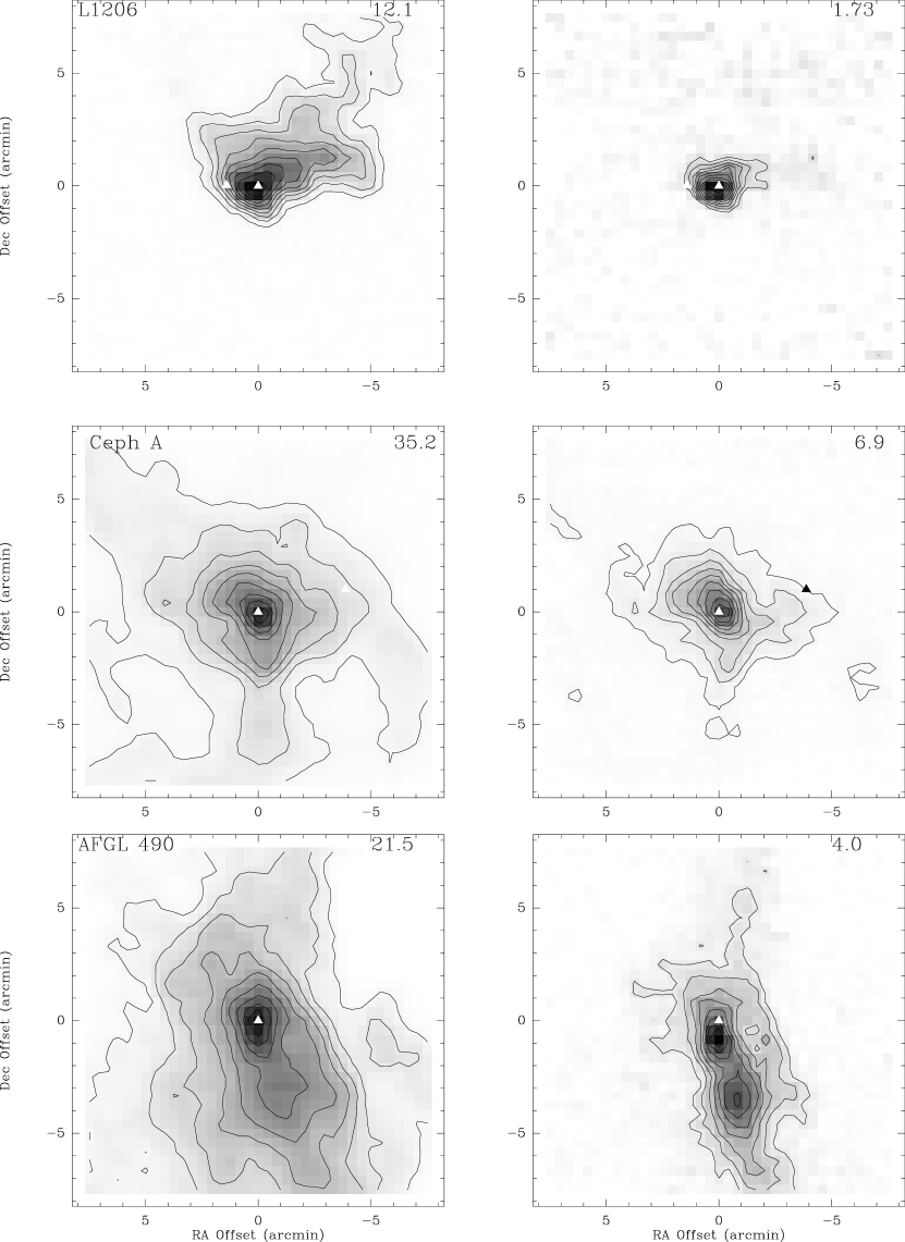
Figure 3: Integrated intensity maps of developmental Class I sources L 1206 (top), Cep A (middle) and AFGL 490 (bottom). The value of the maximum integrated intensity in K  km s^-1 is given in the top right corner of each panel. Left panels show ¹³CO 1–0 integrated emission, with contours at 10% intervals from 10% to 100% of the maximum integrated intensity. Right panels show integrated C¹⁸O 1–0 emission. Base contour is 3$\sigma$, contour interval is 10%, except for L 1206 where contour interval is 1$\sigma$. (0,0) positions are as given in table A ¹³CO and C¹⁸O Survey of the Molecular Gas Around Young Stellar Clusters Within 1 kpc of the Sun. Symbols as in figure 2.

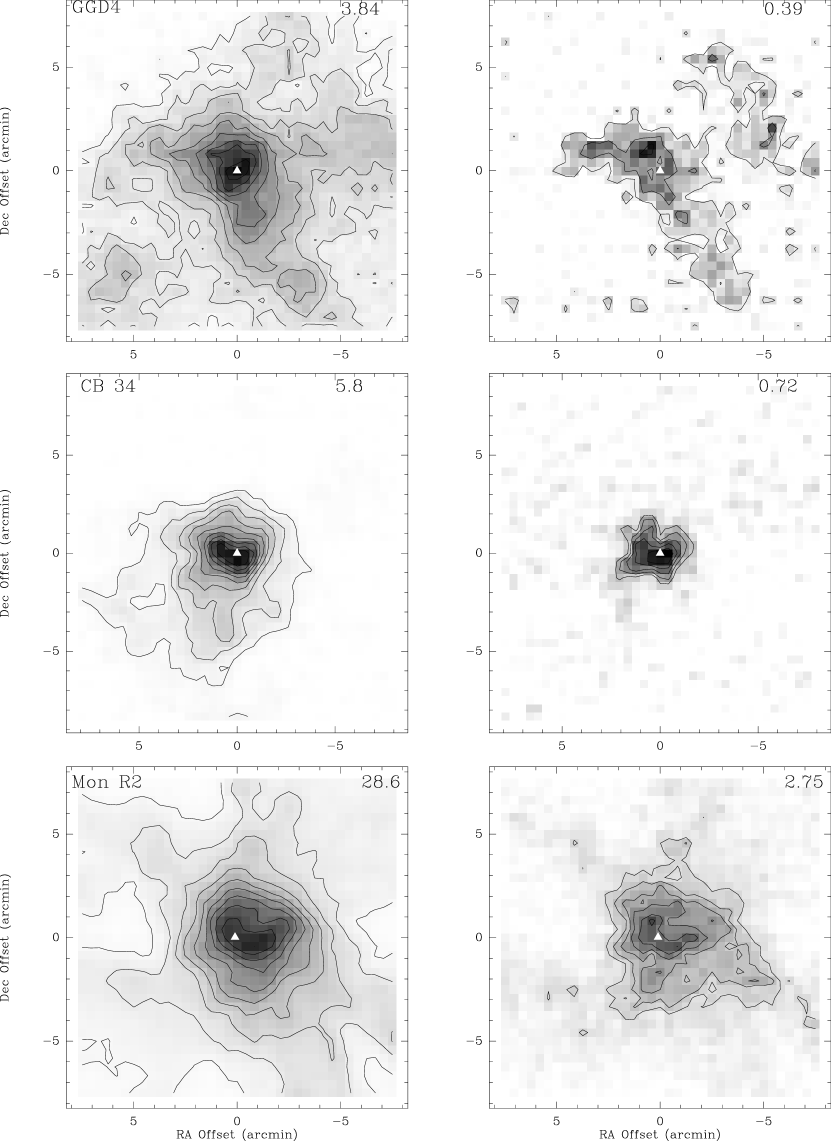
Figure 4: Integrated intensity maps of GGD 4 (top), CB 34 (middle) and Mon R2 (bottom). The value of the maximum integrated intensity in K  km s^-1 is given in the top right corner of each panel. Left panels show ¹³CO 1–0 integrated emission, with contours at 10% intervals from 10% to 100% of the maximum integrated intensity. Right panels show integrated C¹⁸O 1–0 emission. Base contour is 3$\sigma$, contour interval is 1$\sigma$, except for GGD 4 where the base contour is at 1$\sigma$. (0,0) positions are as given in table A ¹³CO and C¹⁸O Survey of the Molecular Gas Around Young Stellar Clusters Within 1 kpc of the Sun. Symbols as in figure 2.

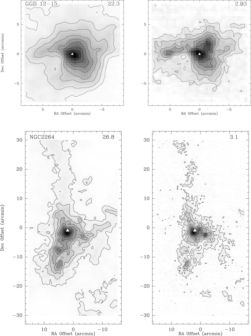
Figure 5: Integrated intensity maps of Class I sources GGD 12-15 (top) and NGC 2264 (bottom). The value of the maximum integrated intensity in K  km s^-1 is given in the top right corner of each panel. Left panel shows ¹³CO 1–0 integrated emission, with contours at 10% intervals from 10% to 100% of the maximum integrated intensity. Right panel shows integrated C¹⁸O 1–0 emission. Base contour is 3$\sigma$ (10% for NGC 2264), contour interval is 1$\sigma$ (10% for NGC 2264). (0,0) positions are as given in table A ¹³CO and C¹⁸O Survey of the Molecular Gas Around Young Stellar Clusters Within 1 kpc of the Sun. Symbols as in figure 2.

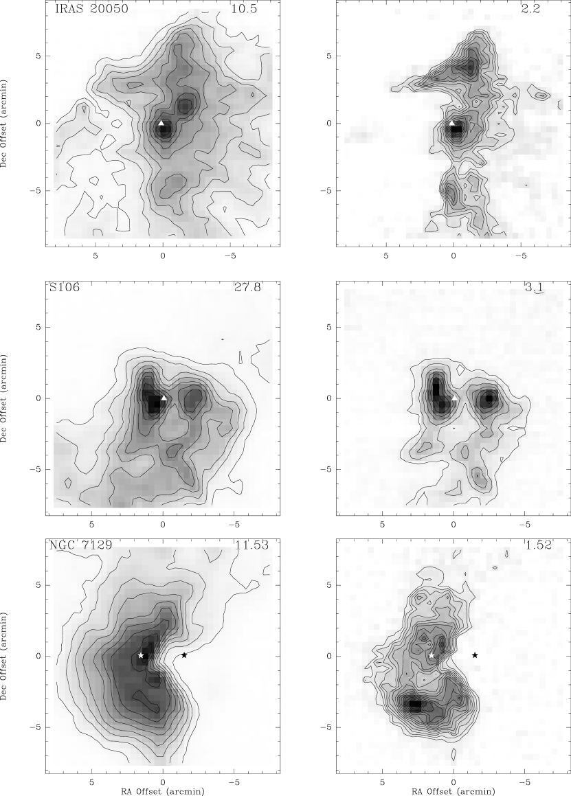
Figure 6: Integrated intensity maps of Class II sources IRAS 20050 (top), S 106 (middle) and NGC 7129 (bottom). The value of the maximum integrated intensity in K  km s^-1 is given in the top right corner of each panel. Left panels show ¹³CO 1–0 integrated emission, with contours at 10% intervals from 10% to 100% of the maximum integrated intensity. Right panels show integrated C¹⁸O 1–0 emission. Base contour is 3$\sigma$, contour interval is 1$\sigma$. (0,0) positions are as given in table A ¹³CO and C¹⁸O Survey of the Molecular Gas Around Young Stellar Clusters Within 1 kpc of the Sun. Symbols as in figure 2.

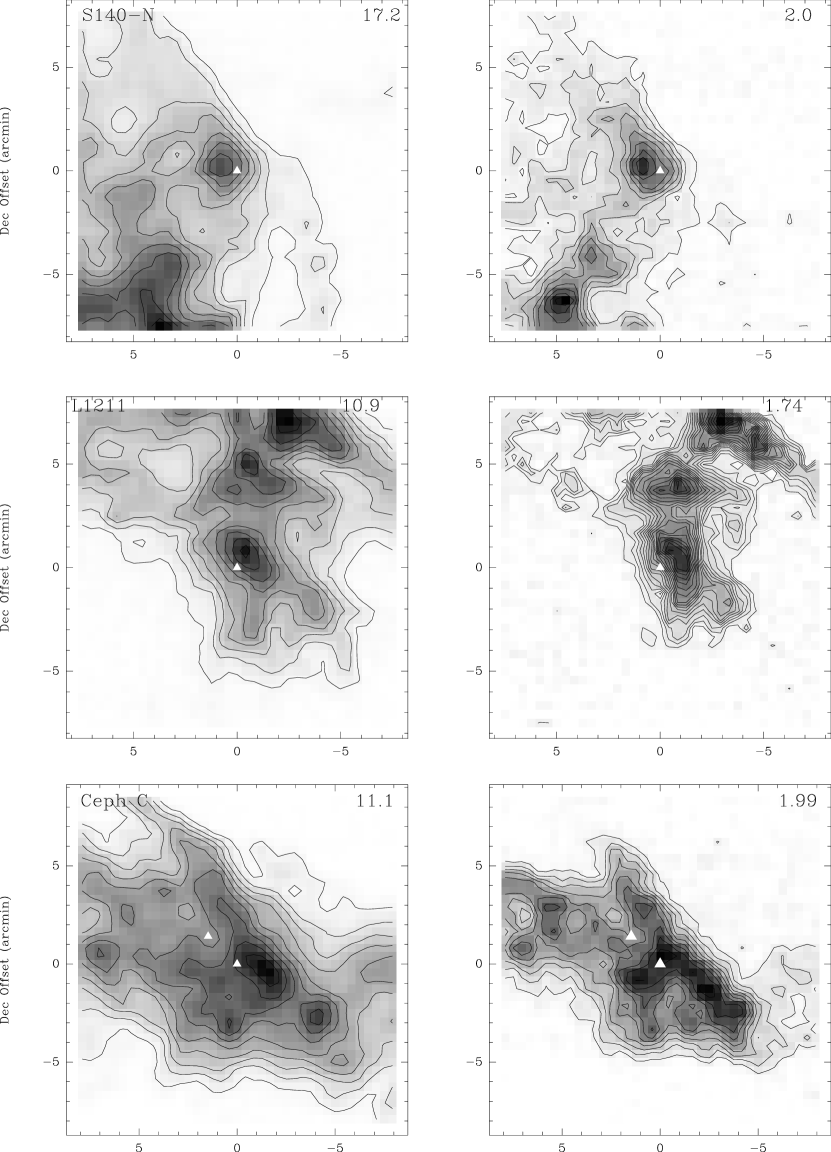
Figure 7: Integrated intensity maps of Class II sources S 140-N (top), L 1211 (middle) and Ceph C (bottom). The value of the maximum integrated intensity in K  km s^-1 is given in the top right corner of each panel. Left panels show ¹³CO 1–0 integrated emission, with contours at 10% intervals from 10% to 100% of the maximum integrated intensity. Right panels show integrated C¹⁸O 1–0 emission. Base contour is 3$\sigma$ (10% for S140-N), contour interval is 1$\sigma$ (10% for S140-N). (0,0) positions are as given in table A ¹³CO and C¹⁸O Survey of the Molecular Gas Around Young Stellar Clusters Within 1 kpc of the Sun. Symbols as in figure 2.

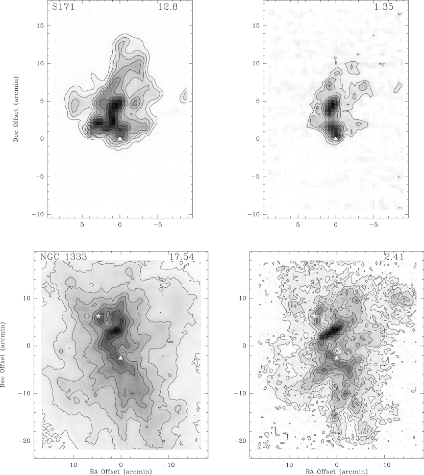
Figure 8: Integrated intensity maps of Class II sources S 171 (top) and NGC 1333 (bottom). The value of the maximum integrated intensity in K  km s^-1 is given in the top right corner of each panel. Left panels show ¹³CO 1–0 integrated emission, with contours at 10% intervals from 10% to 100% of the maximum integrated intensity. Right panels show integrated C¹⁸O 1–0 emission. Base contour is 3$\sigma$, contour interval is 1$\sigma$. (0,0) positions are as given in table A ¹³CO and C¹⁸O Survey of the Molecular Gas Around Young Stellar Clusters Within 1 kpc of the Sun. Symbols as in figure 2.

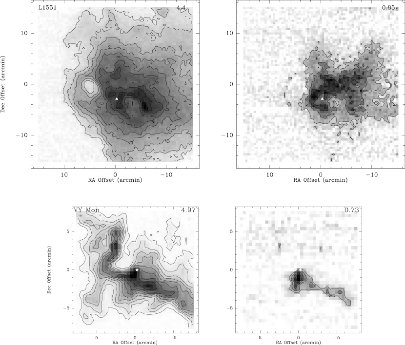
Figure 9: Integrated intensity maps of Class II sources L 1551 (top), and VY Mon (bottom). The value of the maximum integrated intensity in K  km s^-1 is given in the top right corner of each panel. Left panels show ¹³CO 1–0 integrated emission, with contours at 10% intervals from 10% to 100% of the maximum integrated intensity. Right panels show integrated C¹⁸O 1–0 emission. Base contour is 3$\sigma$ (1$\sigma$ for L1551), contour interval is 1$\sigma$. (0,0) positions are as given in table A ¹³CO and C¹⁸O Survey of the Molecular Gas Around Young Stellar Clusters Within 1 kpc of the Sun. Symbols as in figure 2.

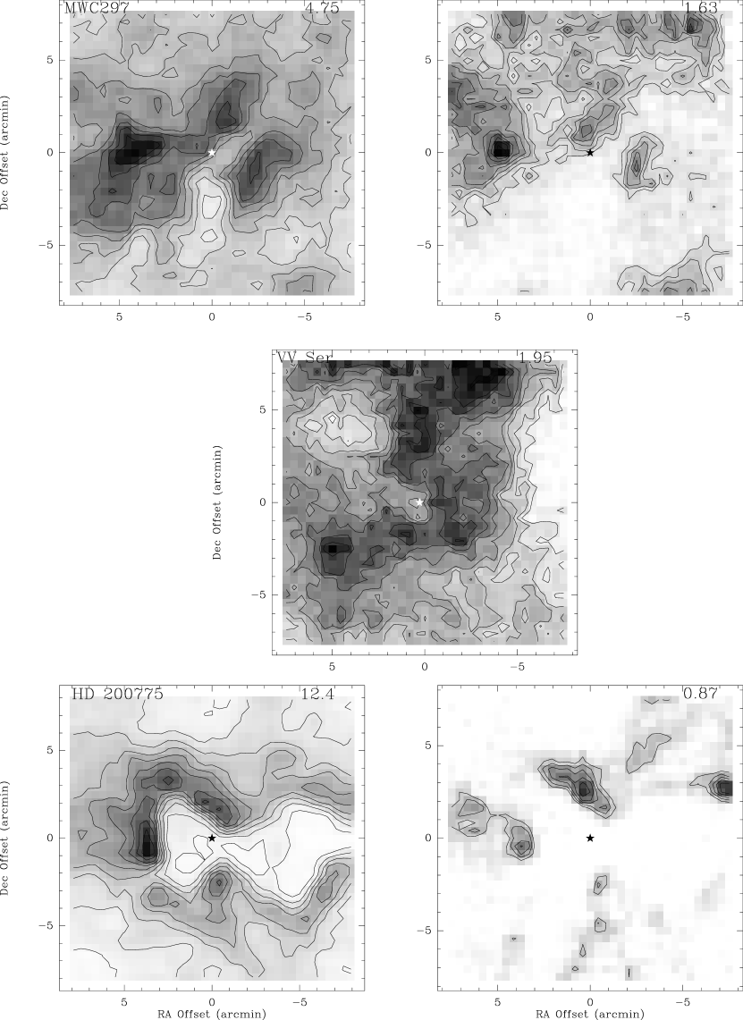
Figure 10: Integrated intensity maps of Class III sources MWC 297 (top), VV Ser (middle) and HD 200775 (bottom). The value of the maximum integrated intensity in K  km s^-1 is given in the top right corner of each panel. Left panels show ¹³CO 1–0 integrated emission, with contours at 10% intervals from 10% to 100% of the maximum integrated intensity. Right panels show integrated C¹⁸O 1–0 emission. Base contour is 3$\sigma$, contour interval is 1$\sigma$. C¹⁸O emission was too weak to map in VV Ser. (0,0) positions are as given in table A ¹³CO and C¹⁸O Survey of the Molecular Gas Around Young Stellar Clusters Within 1 kpc of the Sun. Symbols as in figure 2.

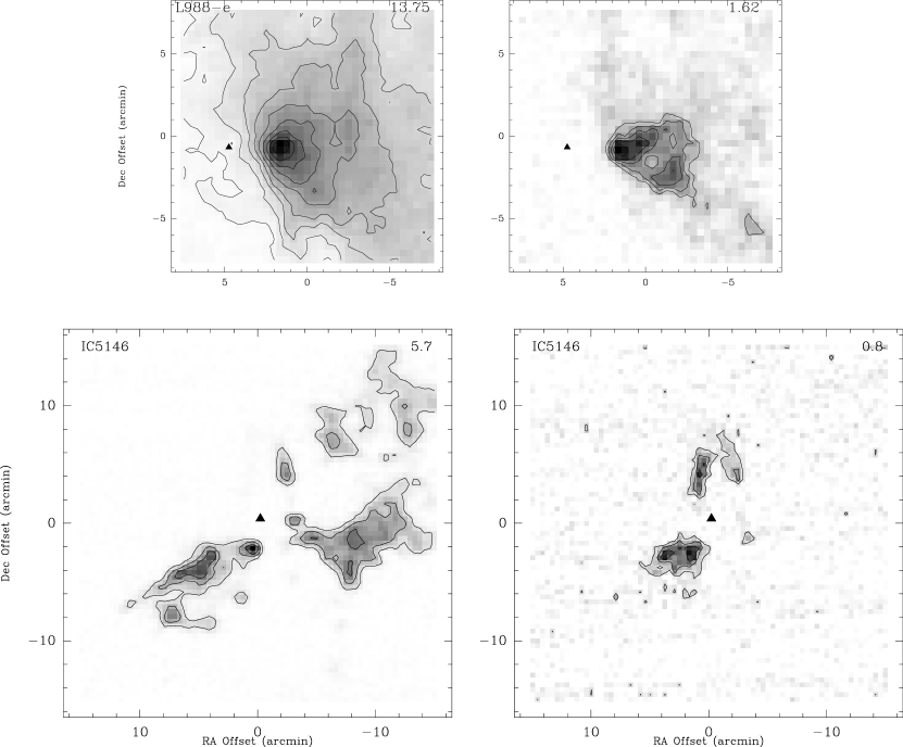
Figure 11: Integrated intensity maps of Class III sources L988-e (top) and IC 5146 (bottom). The value of the maximum integrated intensity in K  km s^-1 is given in the top right corner of each panel. Left panels show ¹³CO 1–0 integrated emission, with contours at 10% intervals from 10% to 100% of the maximum integrated intensity. Right panels show integrated C¹⁸O 1–0 emission. Base contour is 3$\sigma$ (1$\sigma$ for IC 5146), contour interval is 1$\sigma$. (0,0) positions are as given in table A ¹³CO and C¹⁸O Survey of the Molecular Gas Around Young Stellar Clusters Within 1 kpc of the Sun. Symbols as in figure 2.

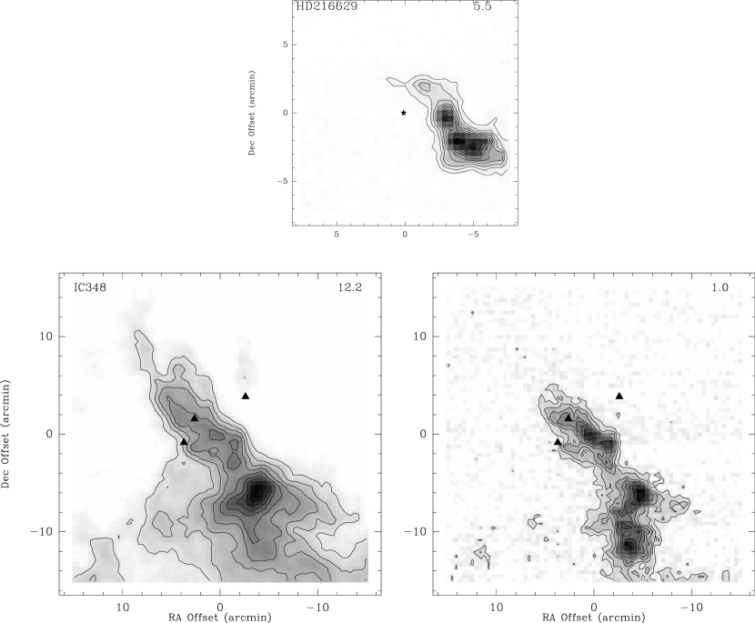
Figure 12: Integrated intensity maps of Class III sources HC 216629 (top) and IC 348 (bottom). The value of the maximum integrated intensity in K  km s^-1 is given in the top right corner of each panel. Left panels show ¹³CO 1–0 integrated emission, with contours at 10% intervals from 10% to 100% of the maximum integrated intensity. Right panels show integrated C¹⁸O 1–0 emission. Base contour is 3$\sigma$, contour interval is 1$\sigma$. (0,0) positions are as given in table A ¹³CO and C¹⁸O Survey of the Molecular Gas Around Young Stellar Clusters Within 1 kpc of the Sun. Symbols as in figure 2.

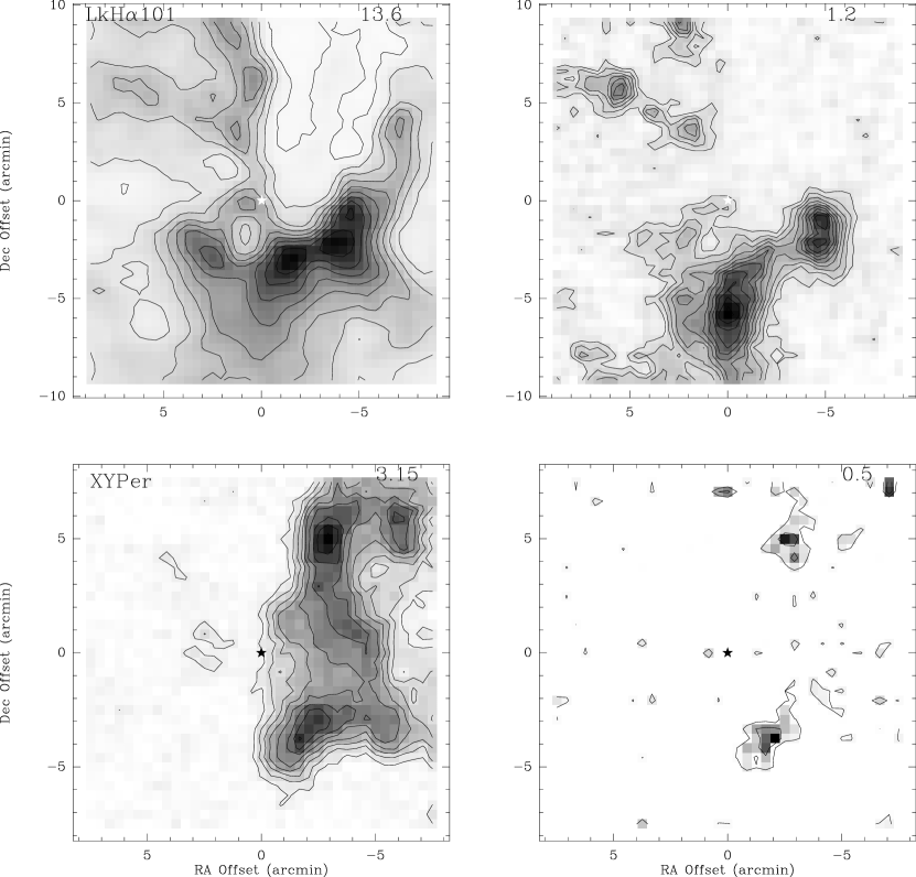
Figure 13: Integrated intensity maps of Class III sources LkH$\alpha$101 (top) and XY Per (bottom). The value of the maximum integrated intensity in K  km s^-1 is given in the top right corner of each panel. Left panels show ¹³CO 1–0 integrated emission, with contours at 10% intervals from 10% (3$\sigma$ for XY Per) to 100% of the maximum integrated intensity. Right panels show integrated C¹⁸O 1–0 emission. Base contour is 3$\sigma$ (1$\sigma$ for XY Per), contour interval is 1$\sigma$. (0,0) positions are as given in table A ¹³CO and C¹⁸O Survey of the Molecular Gas Around Young Stellar Clusters Within 1 kpc of the Sun. Symbols as in figure 2.

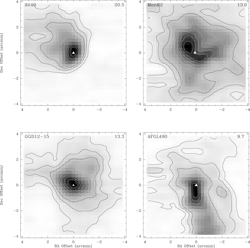
Figure 15: C¹⁸O 2–1 integrated intensity maps of S140, Mon R2, GGD 12-15 and AFGL 490. Base contour is at 10%, contour interval is 10% of the maximum integrated intensity, as given in the top right corner of each panel. (0,0) positions are as given in table A ¹³CO and C¹⁸O Survey of the Molecular Gas Around Young Stellar Clusters Within 1 kpc of the Sun. Symbols are as in figures 2.

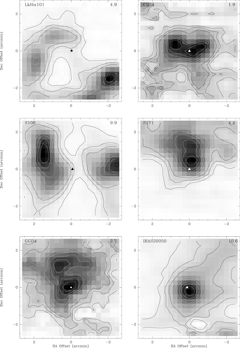
Figure 16: C¹⁸O 2–1 integrated intensity maps of LkH$\alpha$101, CB34, S106, S171, GGD4, and IRAS 20050. Base contour is at 10%, contour interval is 10% of the maximum integrated intensity, as given in the top right corner of each panel. (0,0) positions are as given in table A ¹³CO and C¹⁸O Survey of the Molecular Gas Around Young Stellar Clusters Within 1 kpc of the Sun. Symbols are as in figures 2.

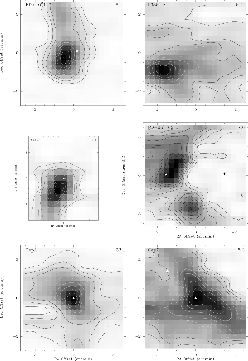
Figure 17: C¹⁸O 2–1 integrated intensity maps of BD+40^∘4124, L988-e, S131, NGC 7129, Cep A and Cep C. Base contour is at 10%, contour interval is 10% of the maximum integrated intensity, as given in the top right corner of each panel. (0,0) positions are as given in table A ¹³CO and C¹⁸O Survey of the Molecular Gas Around Young Stellar Clusters Within 1 kpc of the Sun. Symbols are as in figures 2.

Figure 18: (a) C¹⁸O 1–0 mass vs. ¹³CO 1–0 mass. Solid line indicates the best-fit line with a slope of 0.48$\pm$0.04, indicating that the masses determined from the ¹³CO observations are approximately a factor of two larger. (b) Central C¹⁸O 2–1 mass vs. Central C¹⁸O 1–0 mass. The dashed line indicates a 1:1 relationship. The two most discrepant sources, GGD 12-15 and CepC are marked. (c) Central C¹⁸O 2–1 mass vs. C¹⁸O 1–0 mass. The solid line indicates a best-fit line, with a slope of 0.35$\pm$0.03. (d) Central mass from C¹⁸O 2–1 emission vs. ’total’ mass from the extended ¹³CO 1–0 emission. The solid line indicates the best-fit line with a slope of 0.23$\pm$0.02.

Figure 19: (a) Histograms of ¹³CO 1–0 masses. Left: Expanded scale between 0 and 1000 M_⊙ with bin size of 100 M_⊙. Right: All sources with bin size of 250 M_⊙.

Figure 20: (a) C¹⁸O 1–0 mass vs. distance. Some source names have been shortened for clarity: HD200 = HD 200775; IR = IRAS 20050; BD+40 = BD+40^∘4124; L988 = L 988-e; GGD12 = GGD 12-15. (b) C¹⁸O 1–0 mass vs. FIR luminosity. Source abbreviations as for (a).

Figure 21: (a) Average C¹⁸O 2–1 linewidth vs. average C¹⁸O 1–0 linewidth. Solid line indicates a 1:1 relation. (b) Average C¹⁸O 2–1 linewidth vs. average ¹³CO 1–0 linewidth. The larger scatter is most likely due to optical depth effects in the ¹³CO spectra.

Figure 22: C¹⁸O 1–0 mass vs. C¹⁸O 1–0 virial mass. Circles represent sources with centrally condensed morphologies, while triangles are sources which are extended or diffuse (for which the virial mass is not really applicable). The dashed line indicates the 1:1 relation.

Figure 23: (a) Average C¹⁸O 1–0 linewidth vs. FIR luminosity. Some source names have been abbreviated for clarity: HD200 = HD 200775; IRAS200 = IRAS 20050; BD = BD+40^∘4124; N71 = NGC7129; Lk = LkH$\alpha$101; MW = MWC 297; SN = S 140-N; S13 = S 131. (b) Average C¹⁸O 1–0 linewidth vs. distance.

Figure 24: Size–linewidth relation for the C¹⁸O 1–0 line.

Table 1: The Sample

Source	RA(1950)	Dec(1950)	Adopted Distance	FIR Luminosity	Nstars	Refs.
	hh:mm:ss	dd:mm:ss	pc	L⊙
MWC297 (catalog )	18:25:01.40	$-$03:51:47.0	450	694.2	37	1,2
VVSer (catalog )	18:26:14.30	+00:06:40.0	440	10.7	24	1,2
IRAS20050 (catalog )	20:05:02.00	+27:20:30.0	700	227.1	$\sim$100	3
BD+40∘4124 (catalog )	20:18:43.32	+41:12:11.6	980	1503	$\gtrsim$19	4
S106 (catalog )	20:25:34.00	+37:12:50.0	600	9205	160	5
HD200775 (catalog )	21:00:59.70	+67:57:56.0	600	585.9	9	1,2
L988-e (catalog )	21:02:04.60	+50:03:20.0	700	206.1	45	6
S131 (catalog )	21:38:53.20	+56:22:18.0	900	125.1	$\lesssim$10	7,8
NGC 7129 (catalog )	21:41:47.00	+65:52:45.5	900	1360	29	1,2
IC5146 (catalog )	21:51:36.23	+47:01:54.9	460	90.8	$>$100	17,18
S140 (catalog )	22:17:41.10	+63:03:41.6	900	20560	$\lesssim$16	9
S140-N (catalog )	22:17:51.10	+63:17:50.0	900	194.1	$>$10	9
L1206 (catalog )	22:27:12.20	+63:58:21.0	900	684.4	27	6
L1211 (catalog )	22:45:23.30	+61:46:07.0	750	47.0	$<$245	6
HD216629 (catalog )	22:51:18.40	+61:52:46.0	700	25.0	29	1,2
CepA (catalog )	22:54:20.20	+61:45:55.0	700	13320	$<$580	6
CepC (catalog )	23:03:45.60	+62:13:49.0	700	105.9	$<$110	6
S171 (catalog )	00:01:23.00	+68:17:59.0	850	60.8	$>$10	10
AFGL490 (catalog )	03:23:39.00	+58:36:33.0	700	1167	45	6
NGC1333 (catalog )	03:25:54.98	+31:08:24.1	350	110.0	143	11
IC348 (catalog )	03:41:13.14	+32:00:52.1	320	2.3	$\sim$400	15,19,24
XYPer (catalog )	03:46:17.40	+38:49:50.0	280	3.4	11	1,2,4,12
LkH$\alpha$101 (catalog )	04:26:57.30	+35:09:56.0	280	713.5	$>$100	12,13,16
L1551 (catalog )	04:28:45.14	+18:04:44.3	140	19.1	$\gtrsim$15	20,21
GGD4 (catalog )	05:37:21.30	+23:49:22.0	1000	359.0	10	6
CB34 (catalog )	05:44:02.40	+20:59:22.0	600	13.8	12	14
MonR2 (catalog )	06:05:20.00	$-$06:22:30.0	830	26010	371	15
GGD12-15 (catalog )	06:08:24.50	$-$06:11:12.0	830	5682	134	15
VYMon (catalog )	06:28:21.00	+10:28:15.0	800	387.4	25	1,2
NGC2264 (catalog )	06:38:10.00	+09:40:00.0	800	367.2	360	22,23

Note. — Source details compiled from the literature

References. — 1. Testi et al. 1998; 2. Testi, Palla, & Natta 1999; 3. Chen et al. 1997; 4. Testi et al. 1997; 5. Hodapp & Rayner 1991; 6. Hodapp 1994; 7. Sugitani et al. 1991; 8. Sugitani, Tamura, & Ogura 1995; 9. Evans et al. 1989; 10. Yang & Fukui 1992; 11. Lada, Alves, & Lada 1996; 12. A. Wilson 2002, personal communication; 13. Barsony, Schombert, & Kis-Halas 1991; 14. Alves & Yun 1995; 15. Carpenter 2000; 16. Aspin & Barsony 1994; 17. Lada, Alves, & Lada 1999; 18. Herbig & Dahm 2002; 19. Carpenter 2002; 20. Fridlund, Huldtgren, & Liseau 1997; 21. Carkner et al. 1996; 22. Lada, Young, & Greene 1993; 23. Schreyer et al. 1997; 24. Lada & Lada 1995.

Table 2: Summary of Observations

Source	FCRAO Observations					SMTO Observations
	Map Size	Spectral Resolution	RMS	Lines Observed		Map Size	Spectral Resolution	RMS	Lines Observed
	(arcmin)	(kHz)	(K)			(arcmin)	(kHz)	(K)
MWC297	15$\times$15	25	0.22	13CO 1–0, C18O 1–0		$\cdots$	$\cdots$	$\cdots$	$\cdots$
VVSer	15$\times$15	25	0.25	13CO 1–0, C18O 1–0		$\cdots$	$\cdots$	$\cdots$	$\cdots$
IRAS20050	15$\times$15	25	0.21	13CO 1–0, C18O 1–0		5$\times$5	250	0.20	C18O 2–1
BD+40∘4124	15$\times$15	50	0.12	13CO 1–0, C18O 1–0		5$\times$5	250	0.14	C18O 2–1
S106	15$\times$15	25	0.16	13CO 1–0, C18O 1–0		5$\times$5	250	0.13	C18O 2–1
HD200775	15$\times$15	25	0.22	13CO 1–0, C18O 1–0		$\cdots$	$\cdots$	$\cdots$	$\cdots$
L988-e	16$\times$16	25	0.34	13CO 1–0, C18O 1–0		5$\times$5	250	0.16	C18O 2–1
S131	8$\times$8	25	0.24	13CO 1–0, C18O 1–0		3$\times$3	250	0.11	C18O 2–1
NGC7129	15$\times$15	25	0.17	13CO 1–0, C18O 1–0		5$\times$5	250	0.17	C18O 2–1
IC5146	30$\times$30	25		13CO 1–0, C18O 1–0		$\cdots$	$\cdots$	$\cdots$	$\cdots$
S140	19$\times$18	25	0.20	13CO 1–0, C18O 1–0		7.5$\times$7.5	250	0.19	C18O 2–1
S140-N	15$\times$15	25		13CO 1–0, C18O 1–0		$\cdots$	$\cdots$	$\cdots$	$\cdots$
L1206	15$\times$15	50	0.22	13CO 1–0, C18O 1–0		$\cdots$	$\cdots$	$\cdots$	$\cdots$
L1211	19$\times$18	25	0.22	13CO 1–0, C18O 1–0		$\cdots$	$\cdots$	$\cdots$	$\cdots$
HD216629	16$\times$16	25	0.35	13CO 1–0, C18O 1–0		$\cdots$	$\cdots$	$\cdots$	$\cdots$
CepA	15$\times$15	25	0.22	13CO 1–0, C18O 1–0		5$\times$5	250	0.17	C18O 2–1
CepC	16$\times$16	25	0.17	13CO 1–0, C18O 1–0		5$\times$5	250	0.17	C18O 2–1
S171	18$\times$28	25	0.19	13CO 1–0, C18O 1–0		5$\times$5	250	0.11	C18O 2–1
AFGL490	15$\times$15	50	0.18	13CO 1–0, C18O 1–0		7.5$\times$7.5	250	0.09	C18O 2–1
NGC1333	33$\times$39	50	0.14	13CO 1–0, C18O 1–0		12.5$\times$12.5	250	0.17	C18O 2–1
IC348	30$\times$30	25		13CO 1–0, C18O 1–0		$\cdots$	$\cdots$	$\cdots$	$\cdots$
XYPer	15$\times$15	50	0.28	13CO 1–0, C18O 1–0		$\cdots$	$\cdots$	$\cdots$	$\cdots$
LkH$\alpha$101	15$\times$19	25	0.17	13CO 1–0, C18O 1–0		5$\times$5	250	0.13	C18O 2–1
L1551	30$\times$30	25		13CO 1–0, C18O 1–0		$\cdots$	$\cdots$	$\cdots$	$\cdots$
GGD4	15$\times$15	25	0.20	13CO 1–0, C18O 1–0		5$\times$5	250	0.16	C18O 2–1
CB34	16$\times$16	25	0.18	13CO 1–0, C18O 1–0		5$\times$5	250	0.17	C18O 2–1
MonR2	15$\times$15	25	0.25	13CO 1–0, C18O 1–0		7.5$\times$7.5	250	0.11	C18O 2–1
GGD12-15	15$\times$15	25	0.19	13CO 1–0, C18O 1–0		7.5$\times$7.5	250	0.14	C18O 2–1
VYMon	15$\times$15	50	0.22	13CO 1–0, C18O 1–0		$\cdots$	$\cdots$	$\cdots$	$\cdots$
NGC2264	60$\times$60	25		13CO 1–0, C18O 1–0		$\cdots$	$\cdots$	$\cdots$	$\cdots$

Table 3: Morphological Properties

Source	Morphology	Npeaks	d∗	Developmental
			(pc)	Type
MWC297	diffuse, extended	3	0.25	III
VVSer	diffuse, extended	5	0.25	III
IRAS20050	core + envelope	2	0	II
BD+40∘4124	compact core	1	0	IBRG
S106	compact core	2	0	II
HD200775	cavity	5	0.45	III
L988-e	core + envelope	1	0.50	III
S131	compact core	1	0	IBRG
NGC 7129	core + cavity	1	0	II
IC5146	extended	7	0.12	III
S140	compact core, cometary	1	0	IBRG
S140-N	core + envelope	2	0.2	II
L1206	compact core	1	0	IBRG
L1211	core + envelope	3	0	II
HD216629	compact core	3	0.60	III
CepA	compact core	1	0	I
CepC	extended ridge	2	0.30	II
S171	compact core	2	0.60	II
AFGL490	core + envelope	1	0	I
NGC1333	core + envelope	1	0.6	II
IC348	core + ridge	1	0.75	III
XYPer	extended ridge	2	0.25	III
LkH$\alpha$101	cavity	2	0.25	III
L1551	extended	2	0.06	II
GGD4	compact core	1	0	I
CB34	compact core	1	0	IBRG
MonR2	core + envelope	1	0	I
GGD12-15	core + envelope	1	0	I
VYMon	extended ridge	3	0	II
NGC2264	core + envelope	1	0	I

Table 4: Masses

(1)	(2)	(3)	(4)	(5)	(6)	(7)	(8)
Source	M[13CO 1–0]	Mvirial[13CO 1–0]	M[C18O 1–0]	Mvirial[C18O 1–0]	Mcentral[C18O 1–0]	M[C18O 2–1]	Mvirial[C18O 2–1]
	M⊙	M⊙	M⊙	M⊙	M⊙	M⊙	M⊙
MWC297	169	613	177	171	$\cdots$	$\cdots$	$\cdots$
VVSer	72	1374	18	$\cdots$	$\cdots$	$\cdots$	$\cdots$
IRAS20050	518	1057	275	654	107	113	238
BD+40∘4124	230	264	78	167	59	105	123
S106	801	1919	198	445	136	125	320
HD200775	653	341	73	53	$\cdots$	$\cdots$	$\cdots$
L988-e	806	1224	197	373	136	73	48
S131	10	78	8.3	133	3.4	7.8	67
NGC 7129	977	979	399	372	162	166	152
IC5146	99.3	110	29.8	34.5	$\cdots$	$\cdots$	$\cdots$
S140	1567	1293	771	862	381	430	363
S140-N	1230	721	358	390	$\cdots$	$\cdots$	$\cdots$
L1206	202	298	69	169	$\cdots$	$\cdots$	$\cdots$
L1211	626	514	290	220	$\cdots$	$\cdots$	$\cdots$
HD216629	47	212	$\cdots$	$\cdots$	$\cdots$	$\cdots$	$\cdots$
CepA	1156	844	570	728	309	306	632
CepC	766	1204	625	658	258	119	189
S171	565	874	164	496	69	79	147
AFGL490	920	1655	341	429	264	202	308
NGC1333	1450	1397	401	397	246	183	162
IC348	216	113	37.7	36.6	$\cdots$	$\cdots$	$\cdots$
pXYPer	17	335	6.5	11	$\cdots$	$\cdots$	$\cdots$
LkH$\alpha$101	223	361	45	126	5	10	50
L1551	34.2	47	20.5	15.3	$\cdots$	$\cdots$	$\cdots$
GGD4	323	598	204	364	94	95	311
CB34	55	204	23	124	23	13	85
MonR2	2550	911	1826	948	652	628	462
GGD12-15	1545	1234	745	698	641	335	241
VYMon	282	432	61	196	$\cdots$	$\cdots$	$\cdots$
NGC2264	3988	1517	1664	586	$\cdots$	$\cdots$	$\cdots$

Table 5: Linewidths and Sizes

(1)	(2)	(3)	(4)	(5)	(6)	(7)
Source	$\Delta$V[13CO 1–0]	R[13CO 1–0]	$\Delta$V[C18O 1–0]	R[C18O 1–0]	$\Delta$V[C18O 2–1]	R[C18O 2–1]
	km s-1	pc	km s-1	pc	km s-1	pc
MWC297	1.89	0.68	1.45	0.33	$\cdots$	$\cdots$
VVSer	2.60	0.81	1.19	$\cdots$	$\cdots$	$\cdots$
IRAS20050	2.63	0.61	2.52	0.41	2.44	0.16
BD+40∘4124	1.60	0.41	1.41	0.34	1.46	0.23
S106	4.02	0.47	2.49	0.29	2.31	0.24
HD200775	1.51	0.60	0.81	0.32	$\cdots$	$\cdots$
L988-e	2.94	0.57	1.85	0.44	1.03	0.18
S131	1.27	0.19	1.75	0.17	1.30	0.16
NGC 7129	1.99	0.99	1.46	0.70	1.30	0.36
IC5146	1.1	0.36	0.75	0.25	$\cdots$	$\cdots$
S140	3.02	0.57	2.41	0.59	2.41	0.25
S140-N	1.87	0.83	1.76	0.50	$\cdots$	$\cdots$
L1206	1.70	0.41	1.78	0.21	$\cdots$	$\cdots$
L1211	1.61	0.79	1.29	0.53	$\cdots$	$\cdots$
HD216629	1.60	0.33	$\cdots$	$\cdots$	$\cdots$	$\cdots$
CepA	3.07	0.36	3.28	0.27	3.65	0.19
CepC	2.18	1.01	1.80	0.81	1.47	0.35
S171	2.22	0.71	1.84	0.40	1.40	0.30
AFGL490	3.47	0.55	2.22	0.35	2.10	0.28
NGC1333	2.83	0.69	1.99	0.40	1.80	0.20
IC348	1.3	0.27	0.78	0.24	$\cdots$	$\cdots$
XYPer	2.16	0.29	0.66	0.10	$\cdots$	$\cdots$
LkH$\alpha$101	2.09	0.33	1.48	0.23	1.50	0.09
L1551	0.79	0.30	0.55	0.20	$\cdots$	$\cdots$
GGD4	1.90	0.66	1.59	0.58	1.70	0.43
CB34	1.73	0.27	1.40	0.25	1.37	0.18
MonR2	2.36	0.65	2.26	0.74	2.05	0.44
GGD12-15	2.80	0.63	2.17	0.59	1.89	0.27
VYMon	1.46	0.81	0.98	0.37	$\cdots$	$\cdots$
NGC2264	2.72	0.82	2.15	0.50	$\cdots$	$\cdots$

References

- Adams & Myers (2001) Adams, F. C. & Myers, P. C. 2001, ApJ, 553, 744
- Alves & Yun (1995) Alves, J. F. & Yun, J. L. 1995, ApJ, 438, L107
- Aspin & Barsony (1994) Aspin, C. & Barsony, M. 1994, A&A, 288, 849
- Aspin et al. (1994) Aspin, C., Sandell, G., & Russell, A. P. G. 1994, A&AS, 106, 165
- Bachiller et al. (1995) Bachiller, R., Fuente, A., & Tafalla, M. 1995, ApJ, 445, L51
- Bachiller et al. (1987) Bachiller, R., Guilloteau, S., & Kahane, C. 1987, A&A, 173, 324
- Bally et al. (1996) Bally, J., Devine, D., & Reipurth, B. 1996, ApJ, 473, L49
- Bally & Lada (1983) Bally, J. & Lada, C. J. 1983, ApJ, 265, 824
- Barsony et al. (1991) Barsony, M., Schombert, J. M., & Kis-Halas, K. 1991, ApJ, 379, 221
- Bergin et al. (2002) Bergin, E. A., Alves, J., Huard, T., & Lada, C. J. 2002, ApJ, 570, L101
- Carkner et al. (1996) Carkner, L., Feigelson, E. D., Koyama, K., Montmerle, T., & Reid, I. N. 1996, ApJ, 464, 286
- Carpenter (2000) Carpenter, J. M. 2000, AJ, 120, 3139
- Carpenter (2002) —. 2002, AJ, 124, 1593
- Carpenter et al. (1990) Carpenter, J. M., Snell, R. L., & Schloerb, F. P. 1990, ApJ, 362, 147
- Carpenter et al. (1995) —. 1995, ApJ, 445, 246
- Casoli et al. (1986) Casoli, F., Combes, F., Dupraz, C., Gerin, M., & Boulanger, F. 1986, A&A, 169, 281
- Chen et al. (1997) Chen, H., Tafalla, M., Greene, T. P., Myers, P. C., & Wilner, D. J. 1997, ApJ, 475, 163
- Chini et al. (1991) Chini, R., Henning, T., & Pfau, W. 1991, A&A, 247, 157
- Clark (1986) Clark, F. O. 1986, A&A, 164, L19
- Davis et al. (1998) Davis, C. J., Moriarty-Schieven, G., Eislöffel, J., Hoare, M. G., & Ray, T. P. 1998, AJ, 115, 1118
- Drew et al. (1997) Drew, J. E., Busfield, G., Hoare, M. G., Murdoch, K. A., Nixon, C. A., & Oudmaijer, R. D. 1997, MNRAS, 286, 538
- Eiroa et al. (1993) Eiroa, C., Lenzen, R., Miranda, L. F., Torrelles, J. M., Anglada, G., & Estalella, R. 1993, AJ, 106, 613
- Evans et al. (1989) Evans, N. J., Mundy, L. G., Kutner, M. L., & Depoy, D. L. 1989, ApJ, 346, 212
- Font et al. (2001) Font, A. S., Mitchell, G. F., & Sandell, G. . 2001, ApJ, 555, 950
- Fridlund et al. (1997) Fridlund, M., Huldtgren, M., & Liseau, R. 1997, in IAU Symposium, Vol. 182, 19–28
- Fuente et al. (1998a) Fuente, A., Martin-Pintado, J., Bachiller, R., Neri, R., & Palla, F. 1998a, A&A, 334, 253
- Fuente et al. (2002) Fuente, A., Martín-Pintado, J., Bachiller, R., Rodríguez-Franco, A., & Palla, F. 2002, A&A, 387, 977
- Fuente et al. (1998b) Fuente, A., Martín-Pintado, J., Rodríguez-Franco, A., & Moriarty-Schieven, G. D. 1998b, A&A, 339, 575
- Fukui (1989) Fukui, Y. 1989, in Low Mass Star Formation and Pre-main Sequence Objects, 95
- Fukui et al. (1986) Fukui, Y., Sugitani, K., Takaba, H., Iwata, T., Mizuno, A., Ogawa, H., & Kawabata, K. 1986, ApJ, 311, L85
- Garay et al. (1996) Garay, G., Ramirez, S., Rodríguez, L. F., Curiel, S., & Torrelles, J. M. 1996, ApJ, 459, 193
- Goldsmith et al. (1997) Goldsmith, P. F., Bergin, E. A., & Lis, D. C. 1997, ApJ, 491, 615
- Gomez et al. (1998) Gomez, Y., Lebron, M., Rodriguez, L. F., Garay, G., Lizano, S., Escalante, V., & Canto, J. 1998, ApJ, 503, 297
- Henkel et al. (1986) Henkel, C., Guesten, R., & Haschick, A. D. 1986, A&A, 165, 197
- Herbig & Dahm (2002) Herbig, G. H. & Dahm, S. E. 2002, AJ, 123, 304
- Heyer et al. (2001) Heyer, M. H., Narayanan, G., & Brewer, M. K. 2001, On the Fly Mapping at the FCRAO 14m Telescope, FCRAO
- Hillenbrand (1997) Hillenbrand, L. A. 1997, AJ, 113, 1733
- Hillenbrand et al. (1995) Hillenbrand, L. A., Meyer, M. R., Strom, S. E., & Skrutskie, M. F. 1995, AJ, 109, 280
- Hodapp (1994) Hodapp, K. 1994, ApJS, 94, 615
- Hodapp & Rayner (1991) Hodapp, K. & Rayner, J. 1991, AJ, 102, 1108
- Huard et al. (2000) Huard, T. L., Weintraub, D. A., & Sandell, G. 2000, A&A, 362, 635
- Hughes (2001) Hughes, V. A. 2001, ApJ, 563, 919
- Jijina et al. (1999) Jijina, J., Myers, P. C., & Adams, F. C. 1999, ApJS, 125, 161
- Khanzadyan et al. (2002) Khanzadyan, T., Smith, M. D., Gredel, R., Stanke, T., & Davis, C. J. 2002, A&A, 383, 502
- Kutner & Ulich (1981) Kutner, M. L. & Ulich, B. L. 1981, ApJ, 250, 341
- Lada et al. (1996) Lada, C. J., Alves, J., & Lada, E. A. 1996, AJ, 111, 1964
- Lada et al. (1999) —. 1999, ApJ, 512, 250
- Lada et al. (1993) Lada, C. J., Young, E. T., & Greene, T. P. 1993, ApJ, 408, 471
- Lada (1992) Lada, E. A. 1992, ApJ, 393, L25
- Lada et al. (1991) Lada, E. A., Bally, J., & Stark, A. A. 1991, ApJ, 368, 432
- Lada & Lada (1995) Lada, E. A. & Lada, C. J. 1995, AJ, 109, 1682
- Larson (1981) Larson, R. B. 1981, MNRAS, 194, 809
- Little et al. (1990) Little, L. T., Heaton, B. D., & Dent, W. R. F. 1990, A&A, 232, 173
- MacLaren et al. (1988) MacLaren, I., Richardson, K. M., & Wolfendale, A. W. 1988, ApJ, 333, 821
- Margulis & Lada (1986) Margulis, M. & Lada, C. J. 1986, ApJ, 309, L87
- Margulis et al. (1989) Margulis, M., Lada, C. J., & Young, E. T. 1989, ApJ, 345, 906
- Minchin et al. (1993) Minchin, N. R., White, G. J., & Padman, R. 1993, A&A, 277, 595
- Minier et al. (2001) Minier, V., Conway, J. E., & Booth, R. S. 2001, A&A, 369, 278
- Miskolczi et al. (2001) Miskolczi, B., Tothill, N. F. H., Mitchell, G. F., & Matthews, H. E. 2001, ApJ, 560, 841
- Moriarty-Schieven & Snell (1988) Moriarty-Schieven, G. H. & Snell, R. L. 1988, ApJ, 332, 364
- Oasa et al. (2002) Oasa, Y., Tamura, M., Nakajima, Y., & Itoh, Y. 2002, in The Proceedings of the IAU 8th Asian-Pacific Regional Meeting, Volume II. Edited by S. Ikeuchi, J. Hearnshaw, and T. Hanawa, the Astronomical Society of Japan, p. 189–190
- Ogura et al. (2002) Ogura, K., Sugitani, K., & Pickles, A. 2002, AJ, 123, 2597
- Okada et al. (2002) Okada, Y., Onaka, T., Shibai, H., & Doi, Y. 2002, in Exploiting the ISO Data Archive. Infrared Astronomy in the Internet Age. Edited by C. Gry et al.
- Onishi et al. (1996) Onishi, T., Mizuno, A., Kawamura, A., Ogawa, H., & Fukui, Y. 1996, ApJ, 465, 815
- Palla & Stahler (2000) Palla, F. & Stahler, S. W. 2000, ApJ, 540, 255
- Palla et al. (1995) Palla, F., Testi, L., Hunter, T. R., Taylor, G. B., Prusti, T., Felli, M., Natta, A., & Stanga, R. M. 1995, A&A, 293, 521
- Pirzkal et al. (1997) Pirzkal, N., Spillar, E. J., & Dyck, H. M. 1997, ApJ, 481, 392
- Rodríguez et al. (1999) Rodríguez, L. F., Anglada, G., & Curiel, S. 1999, ApJS, 125, 427
- Rodríguez et al. (1978) Rodríguez, L. F., Moran, J. M., Dickinson, D. F., & Gyulbudagian, A. L. 1978, ApJ, 226, 115
- Rodríguez et al. (1980a) Rodríguez, L. F., Moran, J. M., Gottlieb, E. W., & Ho, P. T. P. 1980a, ApJ, 235, 845
- Rodríguez et al. (1980b) Rodríguez, L. F., Moran, J. M., & Ho, P. T. P. 1980b, ApJ, 240, L149
- Rohlfs & Wilson (2000) Rohlfs, K. & Wilson, T. L. 2000, Tools of Radio Astronomy, 3rd edn. (Springer-Verlag)
- Sargent (1977) Sargent, A. I. 1977, ApJ, 218, 736
- Schneider et al. (2002) Schneider, N., Simon, R., Kramer, C., Stutzki, J., & Bontemps, S. 2002, A&A, 384, 225
- Schreyer et al. (1997) Schreyer, K., Helmich, F. P., van Dishoeck, E. F., & Henning, T. 1997, A&A, 326, 347
- Snell et al. (1984) Snell, R. L., Scoville, N. Z., Sanders, D. B., & Erickson, N. R. 1984, ApJ, 284, 176
- Sugitani et al. (1989) Sugitani, K., Fukui, Y., Mizuni, A., & Ohashi, N. 1989, ApJ, 342, L87
- Sugitani et al. (1991) Sugitani, K., Fukui, Y., & Ogura, K. 1991, ApJS, 77, 59
- Sugitani et al. (1997) Sugitani, K., Morita, K., Nakano, M., Tamura, M., & Ogura, K. 1997, ApJ, 486, L141
- Sugitani et al. (1995) Sugitani, K., Tamura, M., & Ogura, K. 1995, ApJ, 455, L39
- Tafalla et al. (1997) Tafalla, M., Bachiller, R., Wright, M. C. H., & Welch, W. J. 1997, ApJ, 474, 329
- Tafalla et al. (1999) Tafalla, M., Myers, P. C., Mardones, D., & Bachiller, R. 1999, A&A, 348, 479
- Testi et al. (1998) Testi, L., Palla, F., & Natta, A. 1998, A&AS, 133, 81
- Testi et al. (1999) —. 1999, A&A, 342, 515
- Testi et al. (1997) Testi, L., Palla, F., Prusti, T., Natta, A., & Maltagliati, S. 1997, A&A, 320, 159
- Tieftrunk et al. (1998) Tieftrunk, A. R., Megeath, S. T., Wilson, T. L., & Rayner, J. T. 1998, A&A, 336, 991
- Torrelles et al. (1996) Torrelles, J. M., Gomez, J. F., Rodríguez, L. F., Curiel, S., Ho, P. T. P., & Garay, G. 1996, ApJ, 457, L107
- Ungerechts & Thaddeus (1987) Ungerechts, H. & Thaddeus, P. 1987, ApJS, 63, 645
- Urban et al. (2001) Urban, A., Meyer, M. R., Herbig, G. H., & Dahm, S. 2001, American Astronomical Society Meeting, 199
- Watt et al. (1986) Watt, G. D., Burton, W. B., Choe, S.-U., & Liszt, H. S. 1986, A&A, 163, 194
- Wood & Churchwell (1989) Wood, D. O. S. & Churchwell, E. 1989, ApJS, 69, 831
- Wouterloot & Walmsley (1986) Wouterloot, J. G. A. & Walmsley, C. M. 1986, A&A, 168, 237
- Yang & Fukui (1992) Yang, J. & Fukui, Y. 1992, ApJ, 386, 618