The Asiago-ESO/RASS QSO Survey
III. Clustering analysis and its theoretical interpretation

Abstract

This is the third paper of a series describing the Asiago-ESO/RASS QSO survey (AERQS), a project aimed at the construction of an all-sky statistically well-defined sample of relatively bright QSOs ($B\leq 15$) at $z\leq 0.3$. We present here the clustering analysis of the full spectroscopically identified database (392 AGN). The clustering signal at $0.02<z<0.22$ is detected at a $3-4\sigma$ level and its amplitude is measured to be $r_{0}=8.6\pm 2.0h^{-1}$ Mpc (in a $\Lambda CDM$ model). The comparison with other classes of objects shows that low-redshift QSOs are clustered in a similar way to Radio Galaxies, EROs and early-type galaxies in general, although with a marginally smaller amplitude. The comparison with recent results from the 2QZ shows that the correlation function of QSOs is constant in redshift or marginally increasing toward low redshift. We discuss this behavior with physically motivated models, deriving interesting constraints on the typical mass of the dark matter halos hosting QSOs, $M_{\rm DMH}\sim 10^{12.7}h^{-1}M_{\odot}$ ($10^{12.0}-10^{13.5}h^{-1}M_{\odot}$ at 1$\sigma$ confidence level). Finally, we use the clustering data to infer the physical properties of local AGN, obtaining $M_{\rm BH}\sim 2\cdot 10^{8}h^{-1}M_{\odot}$ ($10^{7}-3\cdot 10^{9}h^{-1}M_{\odot}$) for the mass of the active black holes, $\tau_{AGN}\sim 8\cdot 10^{6}$ yr ($2\cdot 10^{6}-5\cdot 10^{7}$ yr) for their life-time and $\eta\sim 0.14$ for their efficiency (always for a $\Lambda CDM$ model).

1 Introduction

The analysis of the statistical properties (luminosity function and clustering) of the cosmic structures is a fundamental cosmological tool to understand their formation and evolution. The clustering of QSOs and galaxies at small to intermediate scales (1-50 $h^{-1}$ Mpc) provides detailed information on the distribution of Dark Matter Halos (DMHs) that are generally thought to constitute the “tissue” on which cosmic structures form. This means to investigate –indirectly– fundamental astrophysical problems, such as the nature of dark matter, the growth of structures via gravitational instability, the primordial spectrum of density fluctuations and its transfer function. The lighting up of galaxies and other luminous objects, such as QSOs, involves complex and non-linear physics. It depends on how the baryons cool within the DMHs and form stars or start accreting onto the central black hole (BH), ending up as the only directly visible peak of a much larger, invisible structure. The so-called bias factor, $b(r,z)$, is used to explain the difference between visible structures and invisible matter, whose gravity governs the overall evolution of clustering. This complex relation is summarized by the simple formula $\xi(r,z)=b^{2}(r,z)\xi_{\rm m}(r,z)$, where $\xi(r,z)$ and $\xi_{\rm m}(r,z)$ are the two-point correlation functions (TPCF) of radiating objects and dark matter, respectively. In this way the detailed analysis of the distribution of the peaks of visible matter can distinguish among the various models for the formation of structures. In particular the hierarchical growth of structures is naturally predicted in a cold dark matter (CDM) scenario, where larger objects are constantly formed from the assembly of smaller ones. An alternative view of the structure formation and evolution, supported by both some observed properties of high-redshift ellipticals and EROs (Daddi et al., 2001, 2002) and theoretical modeling (Lynden-Bell, 1964; Larson, 1975; Matteucci et al., 1998; Tantalo & Chiosi, 2002), leads to the scenario of monolithic collapse, i.e. an earlier object formation and a following passive evolution. The clustering data can be used to discuss whether the merging processes were important at various redshifts or the galaxy number tends to be conserved during the evolution. These two opposite models predict a significantly different redshift evolution of the bias factor (Matarrese et al., 1997; Moscardini et al., 1998).

The first attempt to measure the clustering of QSOs was made by Osmer (1981). Shaver (1984) was the first to detect QSO clustering on small scales using the Véron-Cetty & Véron (1984) catalog, a collection of inhomogeneous samples. A number of authors (Iovino & Shaver, 1988; Andreani & Cristiani, 1992; Mo & Fang, 1993; Shanks & Boyle, 1994; Andreani et al., 1994; Croom & Shanks, 1996) have used complete and better defined QSO samples to measure their spatial distribution. At a mean redshift of $z\sim 1.4$, they generally detect a clustering signal at a typical significance level of $\sim 3-4\sigma$, corresponding to a correlation length, $r_{0}$, similar to the value obtained for local galaxies: $r_{0}\sim 6h^{-1}$ Mpc. However, there has been significant disagreement over the redshift evolution of QSO clustering, including claims for a decrease of $r_{0}$ with redshift (Iovino & Shaver, 1988), an increase of $r_{0}$ with redshift (La Franca et al., 1998) and no change with redshift (Croom & Shanks, 1996). Recently, Croom et al. (2001), using more than 10,000 objects taken from the preliminary data release catalog of 2dF QSO Redshift Survey (hereafter 2QZ), measured the evolution of QSO clustering as a function of redshift. Assuming an Einstein-de Sitter universe ($\Omega_{M}=1.0$ and $\Omega_{\Lambda}=0.0$), they found no significant evolution for $r_{0}$ in comoving coordinates over the redshift range $0.3\leq z\leq 2.9$, whereas for a model with $\Omega_{M}=0.3$ and $\Omega_{\Lambda}=0.7$ the clustering signal shows a marginal increase at high redshift. Here $\Omega_{M}$ and $\Omega_{\Lambda}$ are the mass and cosmological constant density contribution, respectively, to the total density of the universe.

The observed behavior of the QSO clustering can be explained within the linear theory and a typical bias model. The theoretical interpretation of the picture drawn by 2QZ is a result of the combination of many ingredients and their degeneracies: the bias factor, the ratio between the masses of black hole and dark matter halo, the life-time of QSOs, the efficiency and the mass accretion rate.

To add new insights in the modeling and interpretation, one has to consider the constraints from the luminosity function (LF) or/and to enlarge the redshift domain toward lower or higher redshifts. For these reasons, we have started a project, the AERQS, to find bright AGN in the local universe, removing present uncertainties about the properties of the local QSO population and setting the zero point for clustering evolution. For the general aims of the AERQS Survey and its detailed presentation [see Grazian et al. (2000, 2002)].

The goal of this paper is to analyze the clustering properties of a well defined large sample of bright QSOs at $z\leq 0.3$, and provide key information on the following issues: what is the typical mass of DMHs hosting AGN? What is the typical bias factor for AGN? What is the duty cycle for AGN activity? What is the typical efficiency of the central engine at the various redshifts?

The plan of the paper is as follows. In § 2 we describe the data used in the statistical analysis. The various techniques used to investigate the clustering properties are presented in § 3, while § 4 is devoted to a comparison with similar results obtained by previous surveys at low redshifts. To investigate the redshift evolution of the clustering, the spatial properties of QSOs in the local universe are compared in § 5 to the recent 2QZ results at intermediate redshifts for QSOs and to various estimates for normal and peculiar galaxies. In § 6 physically motivated models are used to link the galactic structures at high-$z$ with the local AGN and galaxy population. In § 7 we discuss the clustering properties of QSOs in the light of these simple theoretical models. Finally § 8 gives some concluding remarks on the clustering of QSOs.

2 The Data

It is paradoxical that in the era of 2QZ and Sloan Digital Sky Survey (SDSS), with thousands of faint QSOs discovered up to the highest redshifts, there are still relatively few bright QSOs known at low redshift. One of the main reasons, as shown in previous papers (Grazian et al., 2000, 2002), is the rather low surface density of low-$z$ and bright QSOs, of the order of few times $10^{-2}$ per deg². This corresponds to a very small number of objects also in the case of the 750 deg² of the complete 2QZ and 1000 deg² of the SDSS (during commissioning phase). One more reason, not less important than the previous one, is that with the optical information only it is difficult to efficiently isolate bright QSOs from billions of stars in large areas. As a consequence, a survey based on different selection criteria is required. In Grazian et al. (2000, 2002) we have used the X-ray emission, a key feature of the AGN population.

The AERQS is divided in three sub-samples, two in the northern hemisphere (USNO and GSC), described in Grazian et al. (2000) (hereafter Paper I), and the DSS sample in the southern hemisphere, described in Grazian et al. (2002) (Paper II). After a campaign of spectroscopic identifications at various telescopes, we have completed the sample, which is made up of 392 AGN with redshifts between 0.007 and 2.043. The redshift distributions, shown in Fig. 1, show a peak around $z\sim 0.1$ with an extended tail up to $z=0.4$. Five AGN with $0.6\leq z\leq 2.04$ are possibly objects magnified by gravitational lensing effects. Table 1 summarizes the basic properties of the three sub-samples. The area covered by the AERQS Survey consists of $\sim 14,000$ deg² at the high Galactic latitudes ($|b_{\rm gal}|\geq 30^{\circ}$). The mean values for the completeness and efficiency are 65.7% and 52.3%, respectively.

Table 1: A summary of the AERQS Survey: the three sub-samples.

Name	$DEC$	limit magnitude	Area	$N_{AGN}$	Redshift	Completeness
DSS	$-90\leq\delta\leq 0$	$12.60\leq B\leq 15.13$	5660	111	$0.012\leq z\leq 0.680$	0.63
USNO	$0\leq\delta\leq+90$	$13.50\leq R\leq 15.40$	8164	209	$0.034\leq z\leq 2.043$	0.68
GSC	$0\leq\delta\leq+90$	$12.50\leq V\leq 14.50$	8164	72	$0.007\leq z\leq 0.573$	0.63

Note. — The reported area (in deg²) is the fraction of the northern and southern hemispheres with $|b_{\rm gal}|\geq 30^{\circ}$ and exposure time of the ROSAT All Sky Survey $t_{\rm exp}\geq 300$ sec (as described in Paper I and Paper II).

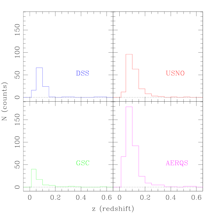
Figure 1: The redshift distributions for the three separated sub-samples (DSS, USNO and GSC) and for the total sample (AERQS, bottom-right panel). Five AGN with higher redshifts (in the range $0.6\leq z\leq 2.04$) are not plotted here.

3 Measuring the Clustering in the AERQS

The simplest way to analyze the clustering properties of a homogeneous and complete sample of QSOs is to compute the TPCF, $\xi(r)$, in the redshift space. We choose to calculate $\xi(r)$ for two representative cosmological models: $(\Omega_{M},\Omega_{\Lambda})=(1.0,0.0)$ and $(0.3,0.7)$. We will call these cosmological models Einstein-de Sitter (hereafter EdS) and $\Lambda$, respectively.

To compute $\xi(r)$ we have used the minimum variance estimator suggested by Landy & Szalay (1993):

$$\xi(r)=\frac{QQ(r)-2QR(r)+RR(r)}{RR(r)},$$ (1)

where $QQ$, $QR$ and $RR$ are the number of QSO-QSO, QSO-random and random-random pairs with a separation $r\pm\Delta r$, respectively. Here $r$ is the comoving distance of two QSOs in the redshift space. We compute the TPCF in bins of $\Delta r=5h^{-1}$ Mpc, where $h$ is the Hubble constant, in units of 100 km s^-1 Mpc^-1. The adopted values for the Hubble constant are $h=0.5$ for the EdS model, and $h=0.65$ for $\Lambda$. We generate 100 random samples and we use the mean values of $QR(r)$ and $RR(r)$ for the estimator.

The correct generation of the random objects is in general the most critical aspect in the clustering analysis. This problem becomes fundamental in the case of a flux-limited sample, the AERQS. The area covered by our survey is not homogeneously distributed in the sky, due to the selection criteria adopted and the variable Galactic extinction. Consequently the “true” apparent magnitude limit of our survey is variable. Fig. 2 shows the effective area covered by the AERQS survey, limited by an exposure time $t_{\rm exp}\geq 300$ sec in the RASS-BSC (Voges et al., 1999) and at high Galactic latitudes ($|b_{\rm gal}|\geq 30^{\circ}$).

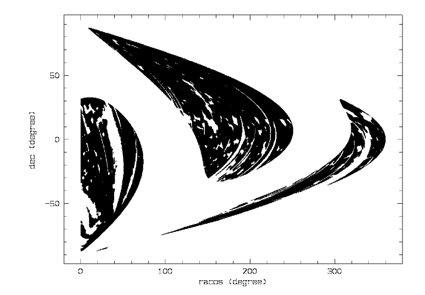
Figure 2: The black area shows the regions covered by the AERQS All Sky Survey after applying the selection criteria described in Paper I and Paper II. The projection is done here in $RA\cos(DEC)$ vs. $DEC$.

The results on clustering reported in this paper are derived by scrambling the redshifts, and the right ascension ($RA$) and declination ($DEC$) coordinates for the total (AERQS) sample. The random $RA$ and $DEC$ are derived from Fig. 2, while the redshifts are randomly extracted from the observed (Gaussian smoothed) redshift distributions (Fig. 1).

In order to check the robustness of the results, we have carried out a more complex generation of random QSOs, which ensured the uniformity of the “synthetic” samples. The angular positions were chosen again randomly from the map in Fig. 2. Then, for each object we generated random values for redshift and absolute magnitude reproducing the LF estimated by La Franca & Cristiani (1997) and Grazian et al. (2000) in the redshift range $0.04\leq z\leq 2.2$. In particular for $\Phi(M_{B},z)$ we adopt a double power-law relation evolving accordingly to a Luminosity Dependent Luminosity Evolution (LDLE) model:

$$\Phi(M_{B},z)={{\Phi^{\ast}}\over{10^{0.4[M_{B}-M_{B}^{*}(z)](\alpha+1)}+10^{0.4[M_{B}-M_{B}^{*}(z)](\beta+1)}}}\ ,\\$$ (2)

where

$$M_{B}^{*}(z)=M^{*}_{B}(z=2)-2.5k\log[(1+z)/3]$$ (3)

and

$$k=k_{1}+k_{2}[M_{B}-M_{B}^{*}(z)]e^{-{z/0.4}} {\rm if}~{}M_{B}\leq M_{B}^{*}(z)$$

$$k=k_{1} {\rm if}~{}M_{B}>M_{B}^{*}(z)\ .$$

The parameters $\alpha$ and $\beta$ correspond to the faint-end and bright-end slopes of the optical LF, respectively, and $M^{*}_{B}(z=2)$ is the magnitude of the break in the double power-law shape of the LF at $z=2$. The actual values adopted in the LDLE parameterization, reported in Tab. 2, are derived by a fit to the observed LF. Extinction by Galactic dust is taken into account using the reddening $E(B-V)$ as a function of position, calculated by Schlegel et al. (1998).

Table 2: The parameters used for the LF of QSOs.

Model	$\Phi^{\ast}$	$M^{*}_{B}(z=2)$	$\alpha$	$\beta$	$k_{1}$	$k_{2}$
EdS	9.8	-26.3	-1.45	-3.76	3.33	0.37
$\Lambda$	5.0	-26.7	-1.45	-3.76	3.33	0.30

Note. — ${\Phi^{\ast}}$ is in units of $10^{-7}$ mag^-1 Mpc^-3.

Table 3: A summary of the clustering properties of the AERQS Sample.

($\Omega_{M}$,$\Omega_{\Lambda}$)	$r_{0}$	$r_{\rm low}-r_{\rm up}$	$\gamma$	$\bar{z}$	$z_{\xi}$	$\bar{\xi}(20)$	$\bar{\xi}_{\rm low}-\bar{\xi}_{\rm up}$	bias
(1.0,0.0)	8.49	6.44–10.46	1.58	0.089	0.063	0.368	0.151–0.585	$1.75\pm 0.51$
(0.3,0.7)	8.64	6.56–10.64	1.56	0.088	0.062	0.461	0.224–0.698	$1.37\pm 0.35$

Note. — The distances are in units of $h^{-1}$ Mpc. The best fit value $r_{0}$ and its 1$\sigma$ confidence level $r_{\rm low}-r_{\rm up}$ are computed from the differential TPCF and the MLE method, assuming a fixed value for the slope $\gamma$. The values $\bar{z}$ and $z_{\xi}$ are the mean redshift of the QSO sample and the median redshift of the observed QSO pairs inside $20h^{-1}$ Mpc, respectively. The value reported in $\bar{\xi}(20)$ is the observed value of the TPCF integrated over $20h^{-1}$ Mpc, with its 1$\sigma$ confidence level, $\bar{\xi}_{\rm low}-\bar{\xi}_{\rm up}$. The bias factor is computed assuming the cosmological parameters described in Section 6.1.

This approach, though computationally expensive, avoids biases in the generation of random samples of QSOs. It reproduces the observed LF and the distribution of redshifts and apparent magnitudes. Fig. 3 shows the observed and random generated QSOs in the $(z,M_{B})$ space in the case of the EdS model.

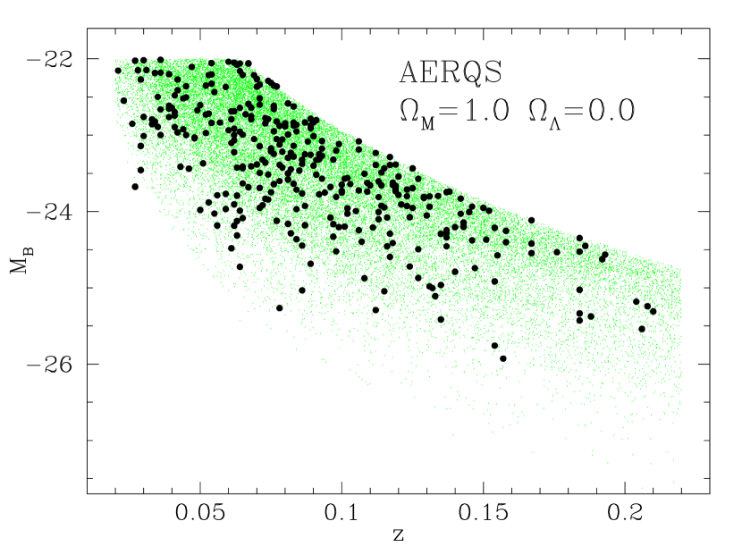
Figure 3: The redshift vs. magnitude $M_{B}$ distribution for the QSOs of AERQS. The observed AGN sample (filled circles) is compared with the random generated sample (small dots) in the $(z,M_{B})$ space. The density of random points is 100 times larger than the observed one. Results are shown for the EdS model.

The results on the clustering of QSOs derived with this particular approach are consistent with the ones obtained with the scrambling of the redshifts. In the following all the computations will be carried out with the latter method.

First, we calculate the TPCF integrated over a sphere, $\bar{\xi}(r)$, as a function of the sphere radius $r$, for the three sub-samples separately (DSS, USNO, GSC) and the total sample (AERQS). Fig. 4 reports the results for the EdS universe, while Fig. 5 refers to a $\Lambda$ universe. The error bars in Fig. 4 and 5 represent the 1$\sigma$ interval for $\bar{\xi}(r)$ and are obtained by assuming a Poisson distribution (Gehrels, 1986).

In order to investigate the possible presence of a spurious clustering signal at large scales, we have computed the angular TPCF binned in intervals of 3 degrees (corresponding to $\sim 14.6h^{-1}$ Mpc comoving). Fig. 6 shows the absence of any significant bias on the large scales sampled by AERQS, up to 150 $h^{-1}$ Mpc.

Figure 4: The integrated correlation function $\bar{\xi}(r)$, as a function of the sphere radius $r$, for an EdS model. Different panels refer to the integrated correlation function (and 1$\sigma$ error bars) for the DSS, GSC, USNO sub-samples, and for the AERQS total sample. $\bar{\xi}(r)$ is integrated over spheres of increasing radii. Consequently the error bars, which are shown only for reference, are not independent. At large scales ($\geq 50h^{-1}Mpc$) the integrated TPCF is consistent with zero, showing the absence of large-scale gradients in the data.

Figure 5: As Fig. 4, but for the $\Lambda$ model.

The signal shown in Fig. 4 and 5 for separations smaller than $15h^{-1}$ Mpc is due to 25 and 28 QSO pairs for the EdS and $\Lambda$ models, respectively. For a completely random distribution, the expected number of pairs is 12 for EdS and 14 for the $\Lambda$ model. Considering separations smaller than $20h^{-1}$ Mpc the observed pairs are 36 and 38, to be compared with 27 and 26 random pairs expected. The clustering signal is therefore detected at a $3-4\sigma$ level.

The differential TPCF for the complete AERQS sample is shown in Fig. 7, both for EdS (upper panel) and $\Lambda$ models (lower panel). The results have been fitted by adopting a power-law relation

$$\xi(r)=\left(\frac{r}{r_{0}}\right)^{-\gamma}\ .$$ (4)

The best-fit parameters can be obtained by using a maximum likelihood estimator (MLE) based on Poisson statistics and unbinned data (Croft et al., 1997). Unlike the usual $\chi^{2}$-minimization, this method allows to avoid the uncertainties due to the bin size (see above), the position of the bin centers and the bin scale (linear or logarithmic).

To build the estimator, it is necessary to estimate the predicted probability distribution of quasar pairs, given a choice for the correlation length $r_{0}$ and the slope $\gamma$. The small number of pairs observed at small scales makes a reliable determination of the slope $\gamma$ particularly difficult. Therefore, we have used fixed values for the slope $\gamma$, adopting those obtained by Croom et al. (2001) for the 2dF catalog, namely $\gamma=1.58$ and $\gamma=1.56$ for EdS and $\Lambda$ models, respectively. In this way, the comparison with the TPCF at higher redshifts obtained from the 2dF data is equivalent both in term of $r_{0}$ and $\bar{\xi}$.

By using all the distances between the quasar-random pairs, we can compute the number of pairs $g(r)dr$ in arbitrarily small bins $dr$ and use it to predict the mean number of quasar-quasar pairs $h(r)dr$ in that interval as

$$h(r)dr={{N_{c}-1}\over{2N_{r}}}[1+\xi(r)]g(r)dr\ ,$$ (5)

where the correlation function $\xi$ is modeled with a power-law as in Eq.(4). In this way, it is possible to use all the distances between the $N_{p}$ quasar-quasar pairs data to build a likelihood. In particular, the likelihood function ${\cal L}$ is defined as the product of the probabilities of having exactly one pair at each of the intervals $dr$ occupied by the quasar-quasar pairs data and the probability of having no pairs in all other intervals. Assuming a Poisson distribution, one finds

$${\cal L}=\prod_{i}^{N_{p}}\exp[-h(r)dr]h(r)dr\prod_{j\neq i}\exp[-h(r)dr]\ ,$$ (6)

where $j$ runs over all the intervals $dr$ where there are no pairs. It is convenient to define the usual quantity $S=-2\ln{\cal L}$, which can be written, once we retain only the terms depending on the model parameter $r_{0}$, as

$$S=2\int^{r_{\rm max}}_{r_{\rm min}}h(r)dr-2\sum_{i}^{N_{p}}\ln[h(r_{i})]\ .$$ (7)

The integral in the previous equation is computed over the range of scales where the fit is made. The minimum scale is set by the smallest scale at which we find QSO pairs ($r_{\rm min}=3h^{-1}$ Mpc), while for the maximum scale we adopt $r_{\rm max}=30h^{-1}$ Mpc. The latter choice is made to avoid possible biases from large angular scales, where the signal is weak.

Figure 6: The differential angular TPCF binned in intervals of 3 degrees (corresponding to $\sim 12.6h^{-1}$ Mpc). Different panels refer to the correlation function (and 1$\sigma$ error bars) for the DSS, GSC, USNO sub-samples, and for the AERQS total sample. These results do not depend on the adopted cosmological model. The angular TPCF at small scales is consistent with zero because it is diluted over 10-20 $h^{-1}$ Mpc.

By minimizing $S$ one can obtain the best-fitting parameter $r_{0}$. The confidence level is defined by computing the increase $\Delta S$ with respect to the minimum value of $S$. In particular, assuming that $\Delta S$ is distributed as a $\chi^{2}$ with one degree of freedom, $\Delta S=1$ corresponds to 68.3 per cent confidence level. It should be noted that by assuming a Poisson distribution the method considers all pairs as independent, neglecting their clustering. Consequently the resulting error bars can be underestimated [see the discussion by (Croft et al., 1997)].

In Fig. 7 the lines represent the 1$\sigma$ confidence region computed with the MLE method previously described, varying only the correlation length $r_{0}$. We find $r_{0}=8.49^{+1.97}_{-2.05}h^{-1}$ Mpc for the EdS model (with $\gamma=1.58$) and $r_{0}=8.64^{+2.00}_{-2.08}h^{-1}$ Mpc for the $\Lambda$ model (with $\gamma=1.56$). The quoted errors on $r_{0}$ are based on the assumption of a fixed slope. It is well known that the errors on $r_{0}$ and $\gamma$ are correlated. Fixing the slopes to $\gamma=1.58$ and 1.56 allows us to derive the confidence levels for the integrated TPCF $\bar{\xi}$ which can be consistently compared with 2QZ results.

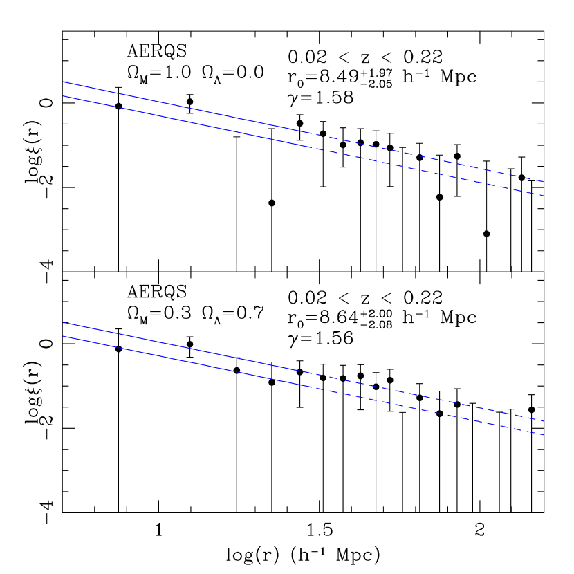
Figure 7: The (differential) two-point correlation function (with 1$\sigma$ error bars) for the AERQS sample in EdS (top panel) and $\Lambda$ models (bottom panel). The solid lines show the 1$\sigma$ confidence region obtained by fitting the data with a power-law relation (with fixed slope) using the MLE approach described in the text. Only points at $r\leq 30h^{-1}$ Mpc are used to fit the TPCF, and they are indicated by the solid line. The dashed line indicates the extension of the TPCF relation to data that are not used for the fit. At small scales ($\log(r)<1.8$) a bin size of $5h^{-1}$ Mpc has been adopted, while at larger scales ($\log(r)\geq 1.8$) a bin sizes of $10h^{-1}$ Mpc has been used. The bin size was chosen too avoid too large bin to bin fluctuations.

It can be useful to present the previous results in a non-parametric form, specified by the clustering amplitude within a given comoving radius, rather than as a scale length which depends on a power-law fit to $\xi(r)$. This is generally represented by the correlation function integrated over a sphere of a given radius in redshift-space $r_{\rm max}$,

$$\bar{\xi}(r_{\rm max})=\frac{3}{r_{\rm max}^{3}}\int_{0}^{r_{\rm max}}\xi(x)x^{2}{\rm d}x\ .$$ (8)

This is the same quantity we plotted in Figs. 4 and 5 for varying $r_{\rm max}$. Different authors have chosen a variety of values for $r_{\rm max}$, e.g. $10h^{-1}$ Mpc (Shanks & Boyle, 1994; Croom & Shanks, 1996), $15h^{-1}$ Mpc (La Franca et al., 1998), or $20h^{-1}$ Mpc (Croom et al., 2001). In general, the larger the scale on which the clustering is measured, the easier the comparison with the linear theory of the structure evolution. Since in the following sections we will compare our results with those obtained for the 2QZ by Croom et al. (2001), we prefer to quote clustering amplitudes within $20h^{-1}$ Mpc, a scale for which linearity is expected to better than a few per cent. Choosing a large radius also reduces the effects of small scale peculiar velocities and redshift measurement errors, which may well be a function of redshift.

Table 3  summarizes the values of $r_{0}$, $\gamma$ and $\bar{\xi}(20)$ for the total sample, both for the EdS and $\Lambda$ models. In the same table, we list the mean redshift ($\bar{z}$) of the observed QSO sample. We also report the median value of the redshift of the QSO pairs computed within a sphere of $20h^{-1}$ Mpc, $z_{\xi}$. We find that it is systematically lower than the mean redshift of the sample.

In our analysis, we do not take into account the velocity field of QSOs, the cone edge effect and the effect of statistical errors on QSO redshifts. Recent papers [see e.g. Croom et al. (2001)] suggest that the Poisson errors, due to the limited size of a sample, are more important than these effects.

4 Comparison with other surveys

It is instructive to compare the present results on the clustering of low-$z$ AGN with that of other surveys, both at low- and high-redshift, in order to get information about the connection between various galactic structures and their evolution. To avoid problems with different assumptions on the values of the slope $\gamma$, we decided to compare the values of the integrated TPCF at 20 $h^{-1}$ Mpc, $\bar{\xi}(20)$. When not directly available in the original paper, $\bar{\xi}(20)$ has been computed by integrating the TPCF with the best fitting values of $r_{0}$ and $\gamma$.

4.1 Comparison with other local AGN surveys

Using a low-redshift ($z\leq 0.2$) sample, Boyle & Mo (1993) measured the clustering properties of 183 AGN in the EMSS. They found evidence for a small value of the integrated TPCF, $\bar{\xi}=0.7\pm 0.6$ (computed at $10h^{-1}$ Mpc), corresponding to a correlation length of $r_{0}=5.0^{+1.9}_{-3.3}h^{-1}$ Mpc. The assumed slope for the TPCF is $\gamma=1.8$ and the resulting $\bar{\xi}(20)$ is $0.20\pm 0.17$. Considering the uncertainties, this result is slightly lower than or consistent with our results. Moreover, since the Boyle & Mo sample is obtained by identifications of X-ray sources, it contains fainter AGN than AERQS. As a consequence, a slightly smaller value of $r_{0}$ is expected for their sample, because the clustering strength is found to depend, weakly, on the absolute magnitude $M_{B}$, as shown in Croom et al. (2002) and in Norberg et al. (2002).

Georgantopoulos & Shanks (1994) investigated the clustering properties of 192 Seyfert galaxies from the IRAS All Sky Survey. They claimed a $2-3\sigma$ detection at $10-20h^{-1}$ Mpc, corresponding to $\bar{\xi}(20)=0.14\pm 0.15$ at $\bar{z}=0.05$, similar to local late-type galaxies. This result is consistent with a model in which local QSOs randomly sample the galaxy distribution.

Carrera et al. (1998) analyzed the clustering of 235 X-ray selected AGN with $0\leq z\leq 3$, obtaining an integrated TPCF of $0.02\leq\bar{\xi}(20)\leq 0.25$. The redshift range of this survey is particularly extended and the density of sources correspondingly low. The clustering detection is marginal, at $2\sigma$ level only. Moreover there are only 33 AGN with $z\leq 0.2$ in this sample.

Akylas et al. (2000) investigated the angular correlation function of 2096 sources selected from the RASS-BSC. They rejected known stars and other contaminants: a cross-correlation analysis with spectroscopic samples indicated that the majority of their sources are indeed AGN. They obtained a $\sim 4\sigma$ detection of clustering. Using the Limber equation and assuming a source redshift distribution (not shown in their paper) with an estimated mean value of 0.1, they derived $\bar{\xi}(20)=0.35\pm 0.09$. Stars, galaxy clusters or other spurious contaminants could affect their results.

Mullis et al. (2001) derived the clustering properties of 217 AGN found in the North Ecliptic Pole (NEP) survey, a connected area of $\sim 81$ deg² covered by ROSAT observations. The sample spans the redshift interval $0\leq z\leq 3.889$, with $\bar{z}=0.408$. A $3.8\sigma$ clustering detection was obtained, corresponding to an integrated TPCF of $\bar{\xi}(20)=0.36\pm 0.15$. This result confirms that X-ray selected AGN are spatially clustered in a manner similar to that of optically/UV selected AGN.

Notice that Boyle & Mo (1993), Georgantopoulos & Shanks (1994), Carrera et al. (1998) and Akylas et al. (2000) used an EdS cosmology to compute the clustering properties of their samples, while Mullis et al. (2001) adopted a $\Lambda$ model.

Finally, it is interesting to compare the clustering properties of AGN and normal galaxies at low-$z$, using our results and recent results by Norberg et al. (2002). Our value for the AGN correlation strength ($\bar{\xi}(20)\sim 0.461\pm 0.237$) appears slightly lower than the typical value for the brighter early-type galaxies ($\bar{\xi}(20)=0.70^{+0.11}_{-0.08}$), or at most consistent, indicating that these two classes have not experienced a completely different evolutionary history, but could represent two distinct phases during the processes of formation and evolution of the same objects. This gives an additional support for models dealing with the joint evolution of QSOs and normal galaxies [e.g. see Haehnelt & Kauffmann (2000); Granato et al. (2001); Franceschini et al. (2002) and references therein]. In particular, the fact that the correlation length of AGN at $z\sim 0$ is consistent with that of ellipticals or S0 in the local universe, reinforces the hypothesis that the QSO host galaxy should be old.

4.2 Comparison with QSO clustering at high-redshift

La Franca et al. (1998) investigated the evolution of QSO clustering using a sample of 388 QSOs with $0.3\leq z\leq 2.2$ over a connected area of 25 deg² down to $B\leq 20.5$ magnitude. Evidence was found for an increase of the clustering with increasing redshift ($\bar{\xi}(20)=0.22^{+0.28}_{-0.18}$ at $0.3\leq z\leq 1.4$ and $\bar{\xi}(20)=0.87^{+0.38}_{-0.21}$ at $1.4\leq z\leq 2.2$). This result does not support the idea of a single population model for QSOs. The general properties of the QSO population studied by La Franca et al. (1998) would arise naturally if QSOs are short-lived events ($\tau\sim 10^{6}-10^{7}$ yr) related to a characteristic halo mass of $\sim 5\cdot 10^{12}M_{\odot}$.

Croom et al. (2001) have used more than 10,000 QSOs taken from the preliminary data release catalog of 2QZ to measure the QSO clustering as a function of redshift. Their sample spans two connected areas for a total of 750 deg² at a limiting magnitude of 20.85 in the $B_{J}$ band. The completely identified sample (not yet released) consists of nearly 22,500 QSOs in the redshift range $0.3\leq z\leq 2.2$. The results from the preliminary data release (to be considered with some caution), expressed in terms of the correlation function integrated inside spheres of $20h^{-1}$ Mpc, $\bar{\xi}(20)$, are shown in Fig. 8, together with the estimates obtained at $z\sim 0.1$ for the AERQS sample. The discussion of the theoretical models shown by the different lines, will be given in the following Section.

For an EdS universe (left panels), Croom et al. (2001) find that there is no significant evolution of the QSO clustering in comoving coordinates over the whole redshift range considered. Assuming a $\Lambda$ model (right panels), the clustering shows a marginal increase at high redshifts, with a minimum of $\xi(r)$ near $z\sim 0.5-1.0$. Our data show a tendency to an increase of $\bar{\xi}(20)$ at low-$z$, both for the EdS and $\Lambda$ models. This result supports the predictions based on simple theoretical models (see next section) and on numerical simulations by Bagla (1998). Notice that very recently this general trend for the clustering evolution has been also confirmed by the power spectrum analysis made by Outram et al. (2003) using the final version of the 2QZ catalog, containing 22,652 QSOs.

The AERQS AGN catalog samples a part of the QSO luminosity function which is fainter than that sampled by the 2QZ. The mean absolute magnitudes of the total AERQS QSOs are $M_{B}=-23.49$ and -22.99 for the EdS and $\Lambda$CDM, respectively. The 2QZ QSOs at $0.3\leq z\leq 2.2$ are brighter than local AGN, with $M_{J}=-24.43$ and -25.11 for EdS and $\Lambda$, respectively. In our comparison, we do not take into account the dependence of the TPCF on the absolute magnitude of the sample, since the QSO population exhibits a strong luminosity evolution with redshift and Croom et al. (2002) have demonstrated that the dependence of the clustering on $M_{B}$ is very weak. A correction of the luminosity dependence of the TPCF would increase the AERQS value, enhancing the redshift evolution of the clustering.

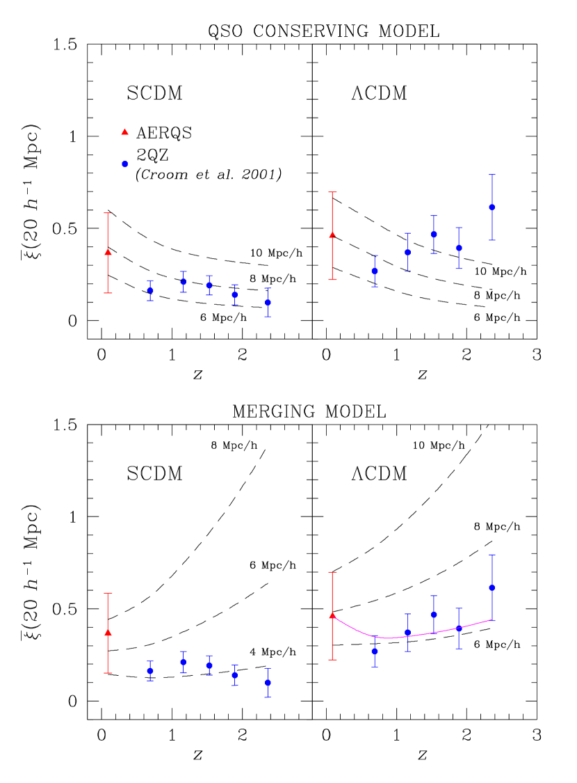
Figure 8: The evolution of the integrated TPCF, $\bar{\xi}(20)$. This plot compares the observational data, shown by points with 1$\sigma$ error bars, to the predicted redshift evolution of the clustering for QSO-conserving (top panels) and merging (bottom panels). The point at $z=0.1$ is our AERQS result, while points at higher redshifts come from 2QZ analysis. Theoretical results for SCDM and $\Lambda CDM$ are shown in the left and right panels, respectively. The dashed lines represent the clustering evolution for models with a given value of the correlation length $r_{0}$ at $z=0$, as indicated in the plot. The solid line in the bottom-right panel refers to the predictions of a combined model, which assumes a merging phase (with $\log M_{\rm min}=12.5$) at high-$z$ and a following conserving phase at low-$z$ (see the text for more details).

5 Modeling the redshift evolution of QSO clustering

By adding the AERQS value of local QSO correlation length to the 2QZ estimates at higher redshifts, we have now the complete picture of the QSO clustering properties up to $z\sim 2.5$, as summarized in Fig. 8. In the following, we introduce a model which can be used to interpret the observed evolution.

In general, the theoretical understanding of how matter clustering grows via gravitational instability in an expanding universe is presently quite well developed, even if the number of ingredients required in the models is large. As a consequence, it is relatively straightforward to compute the correlation function of matter fluctuations, $\xi_{\rm m}$, as a function of redshift, given a cosmological scenario [see e.g. Peacock & Dodds (1996); Smith et al. (2003)]. However, this does not lead directly to a prediction of QSO correlation properties because the details of the link between the distribution of active nuclei and the distribution of the mass are not fully understood. In principle, this relationship could be highly complex, non-linear and environment-dependent, making very difficult to obtain useful informations on the evolution of matter fluctuations from the AGN clustering. In this spirit, a relatively simple form of the local bias $b$ is generally assumed.

Matarrese et al. (1997; see also Moscardini et al. 1998; Hamana et al. 2001) developed an algorithm for describing the clustering on our past light-cone taking into account both the non-linear dynamics of the dark matter distribution and the redshift evolution of the bias factor. The final expression for the observed spatial correlation function $\xi_{\rm obs}$ in a given redshift interval ${\cal Z}$ is

$$\xi_{\rm obs}(r)={\int_{\cal Z}dz_{1}dz_{2}{\overline{\cal N}}(z_{1}){\overline{\cal N}}(z_{2})~{}b_{\rm eff}(z_{1})b_{\rm eff}(z_{2})\xi_{\rm m}(r,\bar{z})\over\bigl{[}\int_{\cal Z}dz_{1}{\overline{\cal N}}(z_{1})\bigr{]}^{2}}\;,$$ (9)

where ${\overline{\cal N}}(z)\equiv{\cal N}(z)/r(z)$, ${\cal N}(z)$ is the actual redshift distribution of the catalog and $r(z)$ describes the relation between comoving radial coordinate and redshift. Here $\bar{z}$ is a suitably defined intermediate redshift. The method has been extended to include the effects of redshift-space distortions using linear theory and the distant-observer approximation (Kaiser, 1987).

A fundamental role in the previous equation is played by the effective bias $b_{\rm eff}$. In fact the final aim of models dealing with clustering is to determine the behavior of the bias factor, once a given theoretical picture is assumed. In practice the effective bias can be expressed as a weighted average of the ‘monochromatic’ bias factor $b(M,z)$ of objects with some given intrinsic property $M$ (like mass, luminosity, etc):

$$b_{\rm eff}(z)\equiv{\cal N}(z)^{-1}\int_{\cal M}d\ln M^{\prime}~{}b(M^{\prime},z)~{}{\cal N}(z,M^{\prime})\,,$$ (10)

where ${\cal N}(z,M)$ is the number of objects actually present in the catalog with redshift within $dz$ of $z$ and property within $d\ln M$ of $\ln M$, whose integral over $\ln M$ is ${\cal N}(z)$.

In most fashionable models of structure formation, the growth of large-scale features happens because of the hierarchical merging of sub-units. Since the development of the clustering hierarchy is driven by gravity, the most important aspects to be understood are the properties of dark halos rather than the QSOs residing in them. Following Mo & White (1996), it is possible to calculate the bias parameter $b(M,z)$ for halos of mass $M$ and ‘formation redshift’ $z_{f}$ observed at redshift $z\leq z_{f}$ in a given cosmological model as

$$b(M,z|z_{f})=1+{1\over\delta_{c}}{D_{+}(z_{f})\over D_{+}(z)}\biggl{(}{\delta_{c}^{2}\over\sigma_{M}^{2}D_{+}(z_{f})^{2}}-1\biggr{)}\;,$$ (11)

where $\sigma^{2}_{M}$ is the linear variance averaged over the scale corresponding to the mass $M$, extrapolated to the present time ($z=0$); $\delta_{c}$ is the critical linear over-density for spherical collapse; $D_{+}$ is the growing factor, depending on the cosmological parameters $\Omega_{M}$ and $\Omega_{\Lambda}$. The distribution in redshift and mass $\bar{n}(z,M)$ for the dark halos can be estimated using the Press & Schechter (1974) formalism; in particular in the following analysis we adopt the relation found by Sheth & Tormen (1999). In the standard treatment of hierarchical clustering, all the halos that exist at a given stage merge immediately to form higher mass halos, so that in practice at each time the only existing halos at all are those which just formed at that time (i.e. $z_{f}=z$). If one identifies quasars with their hosting halos, then the merging rate is automatically assumed to be much faster than the cosmological expansion rate. This is at the basis of what Matarrese et al. (1997) and Moscardini et al. (1998) called merging model. Of course this instantaneous-merging assumption is physically unrealistic and is related to the fact that we use a continuous mass variable, while the aggregates of matter that form are discrete. Assuming a monotone relation between the mass and the observational quantity defining the limits of a given survey, the effective bias can be estimated by considering that the observed objects represent all halos exceeding a certain cutoff mass $M_{\rm min}$ at any particular redshift. In this way, by modeling the linear bias at redshift $z$ for halos of mass $M$ as in equation (11) and by weighting it with the theoretical mass–function $\bar{n}(z,M)$, which can be self–consistently calculated using the Sheth & Tormen (1999) relation, the behavior of $b_{\rm eff}(z)$ is obtained. The parameter $M_{\rm min}$ can be regarded as a free parameter or alternatively fixed in order to obtain given values of the correlation length $r_{0}$ at $z=0$ (see later).

An alternative picture of biasing can be built by imagining that quasar formation occurs at a relatively well-defined redshift $z_{f}$. Actually there are no changes if one assume that there is some spread in the distribution of $z_{f}$. If this is the case, one can further imagine that quasars, which are born at a given epoch $z_{f}$, might well be imprinted with a particular value of $b(M,z_{f})$ as long as the formation event is relatively local. If quasars are biased by birth in this way, then they will not continue with the same biasing factor for all time, but will tend to be dragged around by the surrounding density fluctuations, which are perhaps populated by objects with a different bias parameter. In this case, the evolution of the bias factor can be obtained from (Fry, 1996):

$$b(z)=1+(b_{f}-1){D_{+}(z_{f})\over D_{+}(z)}\;,\\ \\ \\ \\ \\ ~{}z<z_{f}\;,$$ (12)

where $b_{f}$ is the bias at the formation redshift $z_{f}$. Notice that $b(z)$ approaches unity with time, provided that the universe does not become dominated by curvature or vacuum in the meantime (Catelan et al., 1998). This model is called conserving model [see Matarrese et al. (1997) and Moscardini et al. (1998)] or, alternatively, test particle model. Again, it is difficult to motivate this model in detail because it is hard to believe that all galaxies survive intact from their birth to the present epoch, but at least it gives a plausible indication of the direction in which one expects $b$ to evolve if the timescale for quasar formation is relatively short and the timescale under which merging or disruption occurs is relatively long.

Notice that the merging model (rapid merging) and conserving model (no merging) can be regarded as two extreme pictures of how structure formation might proceed. In between these two extremes, one can imagine more general scenarios in which quasars neither survive forever nor merge instantaneously. The price for this greater generality is that one would require additional parameters to be introduced in the models (see the discussion at the end of the next section).

5.1 Results

In the following analysis we will present the results for two different cosmological models. Both models assume a CDM power spectrum (Bardeen et al., 1986), with spectral index $n=1$ and shape parameter $\Gamma=0.2$. The power spectrum normalization (expressed in terms of $\sigma_{8}$, i.e. the r.m.s. fluctuation amplitude in a sphere of $8h^{-1}$ Mpc) is chosen to be consistent with very recent estimates obtained from the cluster abundance analysis [e.g. Reiprich & Böhringer (2002); Viana et al. (2002); Seljak (2002)]. The two considered models are:

• a “standard” CDM Einstein-de Sitter model with $\sigma_{8}=0.5$ (hereafter SCDM);

• a flat CDM universe with ($\Omega_{M}$,$\Omega_{\Lambda})=(0.3,0.7)$ with $\sigma_{8}=0.8$ (hereafter $\Lambda CDM$).

In Fig. 9 we show the redshift evolution of the bias for different values (indicated in the plot in units of $h^{-1}M_{\odot}$) of the minimum mass $M_{\rm min}$ of the halos hosting QSOs. The theoretical predictions are compared to the observational results, shown by the points with 1$\sigma$ error bars. The values at $z=0.1$ represent the bias parameter derived by our analysis of the AERQS. They are obtained by dividing the measured integrated TPCF for QSOs, ${\bar{\xi}}(20)$ by the theoretically predicted autocorrelation function of the underlying matter $\bar{\xi}_{\rm m}(20)$: $b^{2}={\bar{\xi}}(20)/\bar{\xi}_{\rm m}(20)$. We obtain $b=1.75\pm 0.51$ and $b=1.37\pm 0.35$ for SCDM and $\Lambda CDM$, respectively. The data for higher redshifts come from the analysis of the 2QZ survey (Croom et al., 2001).

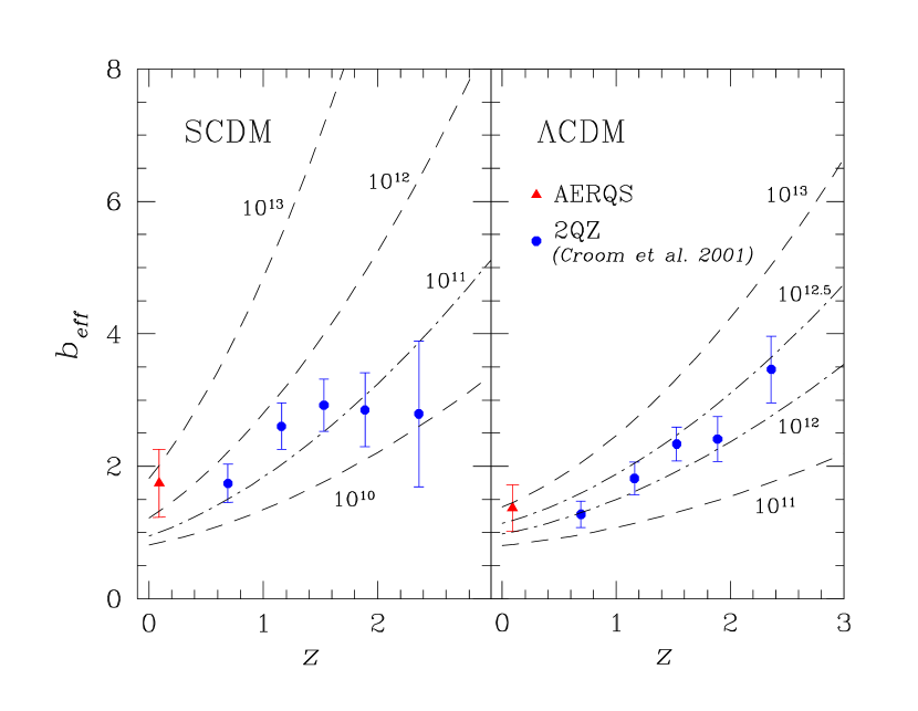
Figure 9: The redshift evolution of the QSO bias factor. The points with 1$\sigma$ error bars represent the observational estimates: the point at $z=0.1$ comes from this analysis of the AERQS catalog, while the remaining data are from 2QZ. The lines show the evolution of the bias obtained assuming different values of the mass $M_{\rm min}$ (in units of $h^{-1}M_{\odot}$).

A first comparison shows that the values for AERQS are consistent with the values at $z\sim 0.7$ for the 2QZ, implying the absence of a significant evolution of bias at low redshifts. As already noticed by Croom et al. (2001), the trend at higher redshifts for bias appears in general to depend on the cosmological models: for $\Lambda CDM$ model, the observed $b$ is always an increasing function of redshift, while in the SCDM case the value of $b$ is almost constant for $z\geq 1.5$.

More interesting is the comparison of the observed $b$ with the theoretical predictions obtained assuming different $M_{\rm min}$. For the $\Lambda CDM$ model the AERQS value corresponds to $\log M_{\rm min}=12.7^{+0.8}_{-0.7}$ (1$\sigma$ error bars), and the observed trend is consistent with the bias evolution expected for dark halos with a minimum mass almost constant in redshift ($\log M_{\rm min}\sim 12-12.5$). On the contrary, for the SCDM model it is impossible to reproduce the bias factor using a constant minimum mass: while the value for AERQS suggests $\log M_{\rm min}=12.5\pm{0.7}$ (always 1$\sigma$ error bars), the bias factor corresponds to halos with $\log M_{\rm min}\sim 11.5$ at $0.5\leq z\leq 1.5$ and $\log M_{\rm min}\leq 11.5$ at $z\geq 2$.

In Fig. 8 we show the predictions for the redshift evolution of the TPCF integrated over $20h^{-1}$ Mpc computed adopting the QSO-conserving (upper panels) and merging (bottom panels) models, described above. The points (with 1$\sigma$ error bars) refer to the observational estimates, again from AERQS at $z=0.1$ and from 2QZ at higher redshifts. The dashed lines represent the results obtained for models built to have given values of the QSO correlation length $r_{0}$ at $z=0$. In particular in the case of the QSO-conserving model, we show results for $r_{0}(z=0)=6,8,10$ $h^{-1}$ Mpc for both models. In the case of the merging model, we show the results for $r_{0}(z=0)=4,6,8h^{-1}$ Mpc, corresponding to a minimum dark matter halo mass of $3.4\times 10^{11},4.6\times 10^{12},1.7\times 10^{13}h^{-1}M_{\odot}$, for SCDM, and for $r_{0}(z=0)=6,8,10h^{-1}$ Mpc, corresponding to $M_{\rm min}=2.5\times 10^{12},1.2\times 10^{13}h^{-1},2.9\times 10^{13}h^{-1}M_{\odot}$ for $\Lambda CDM$.

From the figure, it is evident that in the case of SCDM the QSO-conserving model is more or less able to reproduce the clustering evolution over the whole redshift interval, once a local value of $r_{0}\sim 7h^{-1}$ Mpc is used. The situation is quite different for $\Lambda CDM$, for which the high clustering observed at $z\geq 2$ is not compatible with any trend predicted by the QSO-conserving model: only for $z\leq 1$ the decrease of $\bar{\xi}(20)$ follows the model expectations corresponding to a local value of $r_{0}(z=0)\sim 7h^{-1}$ Mpc.

The comparison of the QSO clustering with the predictions of the merging model shows only marginal agreement on the whole interval $0.0\leq z\leq 2.5$. In particular, for SCDM the observational data are close to the predictions of the model corresponding to a low value of the local clustering, $r_{0}(z=0)\sim 4h^{-1}$ Mpc, while for $\Lambda CDM$ the better agreement is for models corresponding to $r_{0}(z=0)\sim 7h^{-1}$ Mpc, but with large deviations.

As already said, these simple schemes do not exhaust all the possible scenarios through which QSOs might have formed and evolved. For example, it is quite possible that merging could play a different role at different redshifts. Present-day AGN, for example, have clearly not just formed at the present epoch since their observational properties suggest a lack of mergers in the recent past. On the other hand, it is plausible that QSOs at much higher redshifts, say $z\geq 2$, are undergoing merging on the same timescale as the parent halos. This suggests the possible applicability of a model where rapid merging works at high redshifts, but it ceases to dominate at lower redshifts and the bias then evolves by equation (12) until now. In this context it is interesting to note that, while $b_{f}$ is a free parameter in equation (12), it is actually predicted, once the appropriate minimum mass is specified. In fact it corresponds to the bias at the redshift $z_{f}$ when objects stop merging. This model has been introduced by Moscardini et al. (1998), where the resulting relations for the redshift evolution of the bias factor are given. The complete application of this combined model to the present data on quasar clustering is quite difficult because of the size of error bars. Only as an example, for $\Lambda CDM$ we compute the predicted $\bar{\xi}(20)$ by assuming a merging model with $\log M_{\rm min}=12.5$, followed by a conserving phase. The result, shown as solid line in the bottom-right panel of Fig. 8, is in rough agreement with the observational data, indicating that the redshift $z_{f}$, where the transition between the two different regimes occurs, is located at approximately $z_{f}=0.8$. Of course, a validation of this model requires more robust estimates of the QSO clustering properties.

6 Discussion

6.1 Clustering in the local universe

As discussed in the previous paragraphs, there are empirical and theoretical evidences that QSOs are biased with respect to the matter distribution. The results of Boyle & Mo (1993), Georgantopoulos & Shanks (1994), Carrera et al. (1998), Akylas et al. (2000) and Mullis et al. (2001) are consistent, within the uncertainties, with the present results. In general we find that, at low-$z$, AGN have a correlation length of $\sim 8h^{-1}$ Mpc. This value is quite similar to the correlation length of ellipticals, EROs or RGs at $z\sim 0$ and higher than that of spirals or late-type galaxies. Assuming the hierarchical clustering paradigm and the SCDM model, a local correlation length of $\sim 8.5\pm 2h^{-1}$ Mpc corresponds to a population of DMHs with mass larger than $\sim 10^{12.5}h^{-1}M_{\odot}$ ($10^{11.8}-10^{13.2}h^{-1}M_{\odot}$ at a $1\sigma$ confidence level) and a bias parameter of $b\sim 1.7$. The space density of DMHs more massive than this limit is $\rho_{\rm DMH}\sim 3.71\cdot 10^{-3}h^{3}$ Mpc^-3 ($0.63-19.64\cdot 10^{-3}h^{3}$ Mpc^-3 at $1\sigma$), as obtained by applying the Press-Schechter formalism (e.g. Sheth & Tormen 1999). The space density of bright AGN in the local universe is $\rho_{\rm AGN}\sim 5.7\cdot 10^{-7}h^{3}$ Mpc^-3, as inferred by Grazian et al. (2000) using a sub-sample of the AERQS with limiting magnitude $M_{B}=-22.5$. We can thus obtain a rough estimate of the duty-cycle of local AGN, $\tau_{\rm AGN}$ using the simple relation

$$\tau_{\rm AGN}=\frac{\rho_{\rm AGN}}{\rho_{\rm DMH}}\cdot\tau_{\rm H}\ ,$$ (13)

where $\tau_{\rm H}$ is the Hubble time. The duty-cycle of AGN at $z\sim 0.1$ turns out to be $\tau_{\rm AGN}\sim 1.7\cdot 10^{6}$ yr (the 1$\sigma$ confidence region is $3.3\cdot 10^{5}-1.0\cdot 10^{7}$ yr). This result is in good agreement with the one Kauffmann & Haehnelt (2002) obtained by comparing their model to the 2QZ data, and only marginally consistent with the value of $\tau_{\rm QSO}\sim 10^{7}$ yr obtained by Steidel et al. (2002) for QSOs at $z\sim 3$. It is worth noting that both these papers adopt a $\Lambda$ model and $h=0.7$.

If we assume the relation found by Ferrarese (2002), namely

$$M_{\rm BH}\sim 10^{7}M_{\odot}\left(\frac{M_{\rm DMH}}{10^{12}M_{\odot}}\right)^{1.65},$$ (14)

it is possible to infer the mass of active BHs $M_{\rm BH}$ at $z\sim 0.1$. With the values of the AGN DMH mass estimated in our sample, $\log hM_{\rm min}/M_{\odot}=12.5\pm{-0.7}$, we can obtain a rough estimate for $M_{\rm BH}$: $6.7\cdot 10^{7}h^{-1}~{}M_{\odot}$ ($4.7\cdot 10^{6}-9.5\cdot 10^{8}h^{-1}M_{\odot}$ at 1$\sigma$). Assuming an absolute magnitude of $M_{B}=-22.5$ that corresponds to a bolometric luminosity $L_{\rm Bol}=10^{12}L_{\odot}$, one can infer a typical ratio $L/M$ for a local AGN of $1.5\cdot 10^{4}L_{\odot}/M_{\odot}$ ($1.1\cdot 10^{3}-2.1\cdot 10^{5}L_{\odot}/M_{\odot}$). For comparison, the Eddington value is $L/M=3.5\cdot 10^{4}L_{\odot}/M_{\odot}$. In this case an efficiency of $\eta\equiv L/L_{\rm Edd}\sim 0.4$ ($0.03-6.1$) is derived.

For the $\Lambda CDM$ model, the correlation length is $r_{0}=8.6\pm 2.0h^{-1}$ Mpc, which correspond to a DMH mass of the order $\log M_{\rm min}=12.7^{+0.8}_{-0.7}$. Following the same approach carried out for the SCDM model, with an AGN density of $\rho_{\rm AGN}\sim 4.9\cdot 10^{-7}h^{3}$ Mpc^-3 and $\rho_{\rm DMH}\sim 8.12\cdot 10^{-4}h^{3}$ Mpc^-3 ($1.28\cdot 10^{-4}-4.31\cdot 10^{-3}h^{3}$ Mpc^-3 at 1$\sigma$) we derive a slightly longer duty cycle of $\tau_{\rm AGN}\sim 7.9\cdot 10^{6}$ yr ($1.5\cdot 10^{6}-5.0\cdot 10^{7}$ yr) and an efficiency of $4.8\cdot 10^{3}L_{\odot}/M_{\odot}$ ($3.3\cdot 10^{2}-1.0\cdot 10^{5}L_{\odot}/M_{\odot}$), corresponding to $\eta\sim 0.14$ ($0.01-2.8$, at 1$\sigma$). Due to the large error bars on the TPCF, the constraints on the efficiency $\eta$ are not stringent, but give nevertheless an indication of the mean value of the Eddington ratio for local AGN.

AGN in the AERQS sample seem thus to accrete in a sub-Eddington regime, lower than the nearly- or super-Eddington accretion generally assumed for QSOs at high redshifts. High-$z$ QSOs are thought to have relatively small masses, so their extreme luminosities point to a high Eddington ratio (1-10 of the standard value). The direct determination of the Eddington ratio for QSOs at high-$z$ is complicated by a number of difficulties, as discussed by Woo & Urry (2002), who suggest that the true value at $z\geq 1$ is uncertain and dominated by selection effects. At $z\sim 0.1$ they obtain a value $L_{\rm Bol}/L_{\rm Edd}\sim 0.1$, consistent with our result. Bechtold et al. (2003), using Chandra observations of high-redshift QSOs, estimated the BH mass and the Eddington ratio at $3.7\leq z\leq 6.28$ and compared it with the value for local AGN. At high-$z$ QSOs possess masses of the order of $10^{10}h^{-1}~{}M_{\odot}$ and are growing at a mass accretion rate of 0.1 ${\dot{m}}_{\rm Edd}$. At low-$z$ their results are comparable with our values, with $M_{\rm BH}$ between $10^{8}$ and $10^{9}h^{-1}~{}M_{\odot}$ and an Eddington ratio $\eta$ between $10^{-2}$ and $10^{-1}$. From the point of view of the theoretical modeling, Ciotti et al. (2003) were able to reproduce the QSO LF the mass function of local BHs with an Eddington ratio constant and equal to $10^{-1}$ in the redshift range $0\leq z\leq 4$. Haiman & Menou (2000) used an Eddington ratio decreasing from $z=4$ to $z=0$ with a typical value of $10^{-2}-10^{-3}$ at $z\sim 0$.

6.2 Interpreting QSO and galaxy clustering

In a sense, the general picture emerging from the observational data is that the clustering evolution for galaxies is similar to the QSO one: at low-$z$, the correlation length is decreasing from the local value reaching a minimum at $z\sim 1$, then it increases till $z\sim 3-4$. As discussed by Arnouts et al. (1999, 2002), the term “evolution” has not to be considered literally. Given a survey defined by its characteristic limiting magnitude and surface brightness, the galaxies observed at high-$z$ typically have higher luminosities. Therefore, the intrinsic differences of the galaxy properties at different $z$ can mimic an evolution, i.e. the evolution measured in a flux-limited survey is not only due to the evolution of a unique population but can be due to a change of the observed population. The picture emerging from QSO clustering points in the same direction: QSOs are not part of a unique population, due to their short duty-cycle, and are intrinsically related with galaxy evolution.

At this stage, it is important to discuss how the clustering depends on absolute magnitude. Moreover, we should consider how the bias factor changes when the catalog selection effects are considered, i.e. when the theoretical quantities, as the mass $M$, are substituted by the observational ones, such as the luminosity $L$. Chosen one of the previously described models, one will end up with the quantity $b(M,z)$ to be understood as ‘the bias that objects of mass $M$ have at redshift $z$’. The effective bias at that redshift can be written more precisely as (see also Martini & Weinberg 2001)

$$b_{\rm eff}(z)=N(z)^{-1}\int d\ln L\,\Phi_{\rm obs}(L)b[M(L),z]\;,$$ (15)

where $N(z)=\int d\ln L\,\Phi_{\rm obs}(L)$ and $\Phi_{\rm obs}(L)$ is the observed luminosity function of the catalog, i.e. the intrinsic luminosity function multiplied by the catalog selection function, which will typically involve a cut in apparent magnitude, whatever wave-band is being used.

Croom et al. (2002) observed a weak trend of the clustering strength with the magnitude, brighter objects being more clustered. Such a behavior can be understood by focusing on the results obtained in the previous paragraph. The efficiency and the accretion rate for local AGN determine the relation between mass and luminosity, and how they evolve with redshift. As a simple consequence, for QSOs at different epochs, luminosity does not necessarily trace mass. The dependence of clustering strength on the luminosity is thus weaker than the one expected in theoretical models assuming a fixed $M/L$ ratio.

EROs and RGs at $z\sim 1$ have higher correlation amplitude than QSOs at the same redshift; indeed they are following slow or passive evolution. Probably at $z\sim 0$ they will plausibly become the brightest and most massive galaxies inside the clusters. QSOs, instead, show a different evolution for the TPCF: their behavior is consistent with that of a typical merging model at high-$z$ and a passive evolution or object-conserving at low-$z$.

Kauffmann & Haehnelt (2002) explored theoretically the possibility of using the cross-correlation between QSOs and galaxies, $\xi_{QGal}$, to obtain new information on the masses of DMHs hosting QSOs. They used a semi-analytical model in which super-massive BHs are formed and fueled during major mergers. The resulting DMH masses can be in principle used to estimate the typical QSO life-time. In current redshift surveys, like the 2dFGRS or SDSS, these measurements will constrain the life-times of low-$z$ QSOs more accurately than QSO auto-correlation function, because galaxies have much higher a space density than QSOs. As a result, $\xi_{QGal}$ can yield information about the processes responsible for fueling SMBHs.

7 Conclusions

The Asiago-ESO/RASS QSO survey (AERQS), an all-sky complete sample of 392 spectroscopically identified objects ($B\leq 15$) at $z\leq 0.3$, has been used to carry out an extended statistical analysis of the clustering properties of local QSOs.

The AERQS makes it possible to remove present uncertainties about the properties of the local QSO population and fix an important zero point for the clustering evolution and its theoretical modeling. With such a data-set, the evolutionary pattern of QSOs between the present epoch and the highest redshifts is tied down.

On the basis of the (integrated and differential) two-point correlation functions, we have detected a $3-4\sigma$ clustering signal, corresponding to a correlation length $r_{0}=8.6\pm 2.0h^{-1}$ Mpc and a bias factor $b=1.37\pm 0.35$ in a $\Lambda CDM$ model. A similar value of $r_{0}$, but corresponding to $b=1.75\pm 0.51$, is obtained for an Einstein-de Sitter model, confirming previous analysis (Boyle & Mo, 1993; Georgantopoulos & Shanks, 1994; Carrera et al., 1998; Akylas et al., 2000; Mullis et al., 2001). These results shows that low-redshift QSOs are clustered in a similar way to radio galaxies, EROs and early-type galaxies, while the comparison with recent results from the 2QZ at higher redshifts shows that the correlation function of QSOs is constant in redshift or marginally increasing toward low redshifts.

This behavior can be interpreted with physically motivated models, taking into account the non-linear dynamics of the dark matter distribution, the redshift evolution of the bias factor, the past light-cone and redshift-space distortion effects. The application of these models allows us to derive constraints on the typical mass of the dark matter halos hosting QSOs: we have found $\log M_{\rm DMH}=12.7^{+0.8}_{-0.7}$ (the mass is units of $h^{-1}M_{\odot}$), almost independently of the cosmological model. Using the abundance of dark matter halos with this minimum mass and assuming the relation found by Ferrarese (2002) between the masses of dark matter halos and active black holes, from the clustering data we can directly infer an estimate for the mass of the central active black holes and for their life-time, $M_{\rm BH}\sim 2.1\cdot 10^{8}h^{-1}M_{\odot}$ ($1.0\cdot 10^{7}-2.9\cdot 10^{9}h^{-1}M_{\odot}$) and $\tau_{AGN}\sim 7.9\cdot 10^{6}$ yr ($1.5\cdot 10^{6}-5.0\cdot 10^{7}$ yr), respectively. This means that local AGN seem to accrete in a sub-Eddington regime. All these values have been obtained for a $\Lambda CDM$ model; slightly shorter duty cycles are derived for an Einstein-de Sitter model. The time-life of $z\sim 3$ QSOs is $\sim 10^{7}~{}yr$, measured by Steidel et al. (2002). This could be a first indication that QSOs at all epochs have a similar life-time, which does not depend strongly on the Hubble time.

Observational data suggest that most nearby galaxies contain central super-massive black holes, supporting the idea that most galaxies pass through a QSO/AGN phase. However, the different clustering properties, together with the the short lifetimes derived for local AGN, suggest that this phase picks out a particular time in the evolution of galaxies, e.g. epochs of major star formation, interactions or merging. In this way the study of the QSO clustering evolution using extended catalogs helps us to distinguish between a number of possible QSO formation mechanisms.

References

- Akylas et al. (2000) Akylas, A., Georgantopoulos, I. & Plionis, M. 2000 MNRAS 318, 1036
- Andreani & Cristiani (1992) Andreani, P. & Cristiani, S. 1992 ApJ 398, 13
- Andreani et al. (1994) Andreani, P., Cristiani, S., Lucchin, F., Matarrese, S. & Moscardini, L. 1994 ApJ 430, 458
- Arnouts et al. (1999) Arnouts, S., Cristiani, S., Moscardini, L., Matarrese, S., Lucchin, F., Fontana, A. & Giallongo, E. 1999 MNRAS 310, 540
- Arnouts et al. (2002) Arnouts, S., Moscardini, L., Vanzella, E., Colombi, S., Cristiani, S., Fontana, A., Giallongo, E., Matarrese, S. & Saracco, P. 2002 MNRAS 329, 355
- Bagla (1998) Bagla, J. S. 1998 MNRAS 297, 251
- Bagla (1998b) Bagla, J. S. 1998 MNRAS 299, 417
- Bardeen et al. (1986) Bardeen, J.M., Bond, J.R., Kaiser, N. & Szalay A.S. 1986, ApJ 304, 15
- Bechtold et al. (2003) Bechtold, J., Siemiginowska, A., Shields, J., Czerny, B., Janiuk, A., Hamann, F., Aldcroft, T. L., Elvis, M. & Dobrzycki A. 2003 ApJ 588, 119
- Boyle & Mo (1993) Boyle, B. J. & Mo, H. J. 1993 MNRAS 260, 925
- Carrera et al. (1998) Carrera, F. J., Barcons, X., Fabian, A. C., Hasinger, G., Mason, K. O., McMahon, R. G., Mittaz, J. P. D. & Page, M. J. 1998 MNRAS 299, 229
- Catelan et al. (1998) Catelan, P., Matarrese, S. & Porciani, C. 1998 ApJ 502, L1
- Ciotti et al. (2003) Ciotti, L., Haiman, Z. & Ostriker, J. P. in Proceedings of the ESO Workshop “The Mass of Galaxies at Low and High Redshift”. R. Bender and A. Renzini, eds, p. 106
- Croft et al. (1997) Croft, R. A. C., Dalton, G. B., Efstathiou, G., Sutherland, W. J. & Maddox, S. J., 1997 MNRAS 291, 305
- Croom & Shanks (1996) Croom, S. M. & Shanks, T. 1996 MNRAS 281, 893
- Croom et al. (2001) Croom, S. M., Shanks, T., Boyle, B. J., Smith, R. J., Miller, L., Loaring, N. S. & Hoyle, F. 2001 MNRAS 325, 483
- Croom et al. (2002) Croom, S. M., Boyle, B. J., Loaring, N. S., Miller, L., Outram, P. J., Shanks, T. & Smith, R. J. 2002 MNRAS 335, 459
- Daddi et al. (2001) Daddi, E., Broadhurst, T., Zamorani, G., Cimatti, A., Röttgering, H. & Renzini, A. 2001 A&A 376, 825
- Daddi et al. (2002) Daddi, E., Cimatti, A., Broadhurst, T., Renzini, A., Zamorani, G., Mignoli, M., Saracco, P., Fontana, A., Pozzetti, L., Poli, F., Cristiani, S., D’Odorico, S., Giallongo, E., Gilmozzi, R. & Menci, N. 2002 A&A 384, 1
- Davis & Peebles (1983) Davis, M. & Peebles, P. J. E. 1983 ApJ 267, 465
- Ferrarese (2002) Ferrarese, L. 2002 ApJ 578, 90
- Franceschini et al. (2002) Franceschini, A., Braito, V. & Fadda, D. 2002 MNRAS 335, 51
- Fry (1996) Fry, J. N. 1996 ApJ 461, L65
- Gehrels (1986) Gehrels, N. 1986 ApJ 303, 346