Abstract

Weak gravitational lensing has the potential to select clusters independently of their baryon content, dynamical state, and star formation history. We present steps toward the first shear-selected sample of clusters, from the Deep Lens Survey (DLS), a deep $BVRz^{\prime}$ imaging survey of 28 square degrees. Cluster redshifts are determined from photometric redshifts of members and from lensing tomography, and in some cases have been confirmed spectroscopically. DLS imaging data are also used to derive mass-to-light ratios, and upcoming Chandra and XMM time will yield X-ray luminosities and temperatures for a subsample of 12 clusters. Thus we can begin to address any baryon or luminous-matter bias which may be present in current optical and X-ray samples. When the DLS is complete, we expect to have a sample of $\sim 100$ shear-selected clusters from $z\sim 0.2-1$.

Chapter 0 Shear-selected clusters from the
Deep Lens Survey

1 Introduction

Already in 1937 F. Zwicky (Zwicky 1937) found that clusters of galaxies are mostly composed of dark matter, yet all cluster catalogs to date have been based on detection of the luminous, baryonic, component of clusters, which is a small fraction of the total matter. Two recently developed methods based on cluster effects on the background have the potential to change that. The Sunyaev-Zel’dovich effect (SZE) method, based on the upscattering of cosmic microwave background photons by the intracluster medium, will select clusters independent of their star formation history, but still depends on baryon content and temperature (Birkinshaw 2003, Romer 2003). Weak gravitational lensing, in which background galaxy images are sheared by the mass of an intervening cluster, will select clusters independent of star formation history, baryon content, and dynamical state.

While each technique has its strengths and weaknesses, we note that the use of clusters as tracers of large-scale structure, and thus as indicators of cosmological parameters such as $\Omega_{m}$ and $\sigma_{8}$, hinges on their mass function, not merely on their number density. Thus it is crucial to compile samples which reflect purely the mass function, with no dependence on star formation history or dynamical state. Shear-selected samples come close to that ideal. Any difference between shear-selected and traditional samples will also be interesting for those who study clusters as systems in their own right.

Here we present steps toward the first shear-selected sample of clusters, using 12 deg² of the Deep Lens Survey (DLS). Because many of the clusters have not yet been assigned redshifts or followed up in other ways, in this paper we concentrate on techniques and examples rather than aggregate features of the sample.

2 Data

The DLS is a deep multicolor (BVRz^′) imaging survey of 28 deg² being carried out at the 4-m telescopes of the US National Observatories (KPNO and CTIO). Over the course of the survey, seven separate $2^{\circ}$ by $2^{\circ}$ fields will be imaged in B, V, R, and z^′ to a limiting surface brightness (1$\sigma$) of approximately 29, 29, 29, and 28 mag arcsec^-2, respectively. The $R$ filter is used when the seeing is 0.9^′′ or better, to optimize its utility for lensing studies. The other filters provide color information for photometric redshift estimates, and are observed when the seeing is worse than 0.9^′′.

The survey has been awarded approximately 100 dark nights and as of now 75% of the observations have been completed. More details about the DLS can be found in this proceedings (Margoniner et al. 2003) or at: http://dls.bell-labs.com.

For a uniform data set, we chose 12 deg² which had total $R$ exposure times of at least 13,500 seconds as of March 2002. Some of this area does not yet have $BVz^{\prime}$ coverage, so only the $R$ data are used for cluster detection in this paper. Where $BVz^{\prime}$ data are available, they may be used to assign redshifts to detected clusters.

3 Mass Maps

From the stacked $R$ images (see Wittman et al. 2002 for details on the image processing), we make preliminary catalogs using SExtractor (Bertin & Arnouts 1996). These are used as input to the ellipto software described in Bernstein & Jarvis (2002), which measures weighted moments of each object. Available subfields (40’ on a side, roughly the size of the camera) within each 2^∘ field are stitched together to make one large catalog covering anywhere from 1 deg² (for fields with only two available subfields) up to 4 deg² (for fields with all subfields available). In the stitching process, multiple measurements of objects in the overlap areas between subfields are compared, and discrepant objects thrown out. The fraction of objects thrown out this way is small, indicating good uniformity across subfields.

To derive a clean, high-median-redshift subcatalog for each field, we select sources with the following properties: (1) ellipto errorcode of zero, (2) SExtractor flags $<4$ (i.e. split objects allowed, but nothing with a reall error), (3) ellipto size $>1.2$ times the point-spread function (PSF) size, because sources must be resolved to show a lensing signal (4) $23<R<25$, to eliminate low-redshift galaxies without going so faint as to include noise objects, (5) ellipto size $<25$ pixel², also to eliminate low-redshift (higher angular diameter) galaxies, and (6) observed ellipticity $<0.5$, because with $\sim 1^{\prime\prime}$ resolution, highly elliptical objects are quite likely to be blends of two distinct sources, based on our measurements of the Hubble Deep Field and synthetic fields convolved with this seeing.

We then make two types of maps based on these catalogs. The first is simply a convergence (i.e., projected mass surface density times a quantity involving distances of sources and lenses) map based on the algorithm of Fischer & Tyson (1997). The second map is a modification of the Fischer & Tyson algorithm, with one less power of $r$ in the kernel, which roughly represents projected potential rather than mass. This second map serves as a sanity check for the first; requiring that they appear on both types of maps reduces the false detection rate. In our simulations, we have found that we can detect clusters as small as 500 km s^-1 equivalent velocity dispersion over the redshift range 0.2–0.7 using this technique. The highest shear clusters in our sample have equivalent velocity dispersions of about 900 km s^-1, and they can be easily seen on both maps.

Finally, tests of shear systematics and $RMS$ noise are made. The first test consists of rotating by $45^{\circ}$ the ellipticities of all sources. Because lensing does not affect this component of ellipticity, the resulting “mass” map gives some indication of noise and systematic errors. The highest peaks on these maps are far below those of the clusters. The second test is the construction of a map from randomized positions (i.e. the xy position of one object becomes the position of another, which preserves any systematics which might come from exclusion zones or the like, while nulling any real lensing signal). Here again, the highest peaks are much lower than on the real mass map.

Figure 1 shows the mass map and its corresponding randomized map for a single 4 deg² DLS field, which is not yet imaged to full depth. Approximately $122$K sources were used in the construction of these $2^{\circ}\times 2^{\circ}$ maps. We expect to double the number of sources, decreasing the noise by $\sim\sqrt{2}$, when full-depth is achieved. In this field, the peak at upper left is in our Chandra sample; the other two obvious peaks would have qualified for the sample, but were not in the 12 deg² available at the time. These two candidates will be in a second Chandra proposal extending the area covered. Other peaks may be noise; judgement will be reserved until after the field is imaged to full depth.

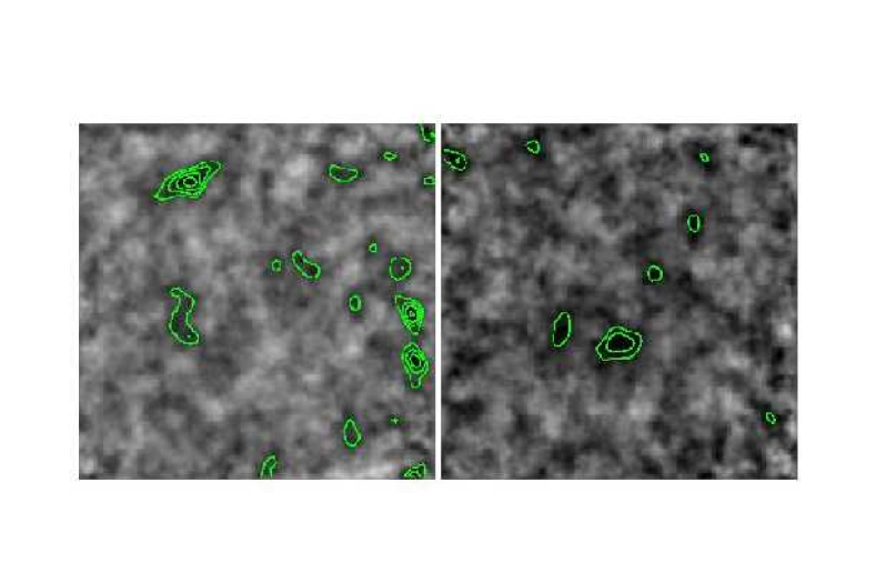
Figure 1: Mass (left) and randomized (right) maps for DLS field F3. The contours indicate positive detections and indicate the same levels in both maps. North is Up, East is to the Left.

4 Photometric Redshifts

The multiband ($BVRz^{\prime}$) DLS observations allows us to estimate photometric redshifts for $\sim 40$ galaxies per square arc min. Our technique is based on SED fitting and on a luminosity function prior. From the comparison between the observed colors of an object and the colors expected from different galaxy types at a range of redshifts, a probability distribution, $pc(z)$, is derived. To compute $pc(z)$ we use the publicly available HyperZ code (Bolzonella et al. 2000). We then compute the probability that an object of apparent magnitude $m$ is at redshift $z$, $pm(z)$, assuming a Schechter luminosity function and taking into account the volume element at $z$ (Peebles 1980). The product of $pc(z)$ and $pm(z)$ generates a final probability distribution from which we determine our photometric redshift (called BestZ) and its uncertainty. Figure 2 shows an example of such probabilities for a galaxy in the DLS with spectroscopic redshift and type determined by Cohen et al.(1999).

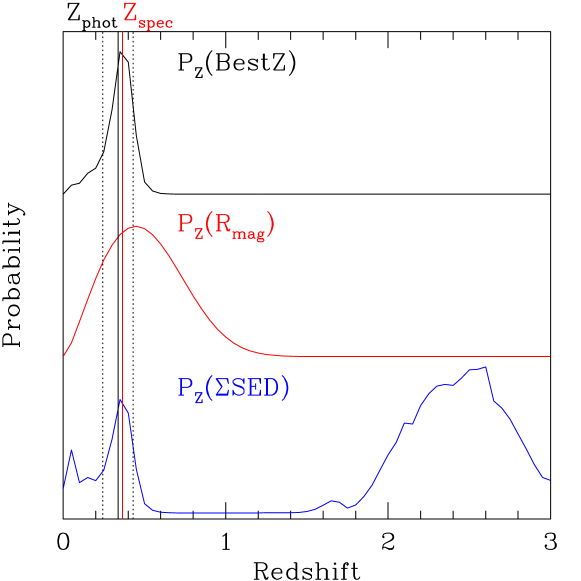
Figure 2: This galaxy, classified as IE by Cohen et al.(1999) and found to be at redshift 0.364, has $R=20.9$ and a photometric redshift $BestZ=0.337\pm 0.094$

Because of the limited number of filters in the DLS, and its relatively small wavelength range, the inclusion of a magnitude prior improves significantly the photometric redshifts estimates from HyperZ alone. To illustrate this, Figure 3 shows spectroscopic (from Cohen et al. 2000) versus photometric redshifts for 119 galaxies in the HDFN, using as input photometry only a limited filter set which roughly simulates the DLS (f450w, f606w, f814w, J). The left panel shows HyperZ estimates, and the right panel shows our BestZ results. We quote our errors in terms of $1+z$: $\Delta_{100\%}=(z_{spec}-z_{phot})/(1+z_{spec})$ takes into account all objects; and $\Delta_{95\%}$ exclude the 5% worst of outliers (as is often done in the literature). In each case, we quote a mean, which represents any overall bias, and an rms, which is the expected error for a single galaxy.

Figure 3: Photometric redshifts based on 4 bands (f450w, f606w, f814w, J) photometry of 119 galaxies in the HDFN. The left panel shows HyperZ results ($\Delta_{100\%}=-0.13\pm 0.59$, $\Delta_{95\%}=-0.03\pm 0.37$); The right panel shows our BestZ results ($\Delta_{100\%}=-0.05\pm 0.25$, $\Delta_{95\%}=-0.00\pm 0.14$).

Figure 4 shows photometric redshifts based on the 7-band (f300w, f450w, f606w, f814w, J, H, K) photometry available for the HDFN galaxies (Fontana et al. 2000). The left panel shows the often mentioned Fontana et al. 2000 results; the middle panel shows HyperZ estimates, and the right panel shows our BestZ estimates. In this case, the HyperZ estimates are nearly as good as BestZ, indicating that the luminosity function prior is not necessary with an extensive filter set. At the same time, it demonstrates that our approach works well in general; the larger per-galaxy errors in the DLS are a result of the limited filter set, not the algorithm. We note that the limited DLS filter set was a conscious choice, as the per-galaxy noise in lensing is already limited by the random orientation of each galaxy (shape noise).

Figure 4: Photometric redshifts based on 7 band photometry of 119 galaxies in the HDFN. The left panel shows Fontana et al.  2000 estimates ($\Delta_{100\%}=0.02\pm 0.13$, $\Delta_{95\%}=0.03\pm 0.06$); the middle panel shows HyperZ results ($\Delta_{100\%}=0.01\pm 0.12$, $\Delta_{95\%}=0.01\pm 0.06$); and the right panel shows our BestZ results ($\Delta_{100\%}=0.00\pm 0.11$, $\Delta_{95\%}=0.00\pm 0.06$).

DLS subfield F1p22 contains the Caltech Faint Galaxy Redshift Survey (CFGRS, Cohen et al. 1999). After excluding stars, quasars, and anything with bad quality factor (quality>6) (see Cohen et al. 1999) we were left with 275 galaxies with reliable redshift measurements and DLS photometry. Figure 5 shows our results. From this analysis we can infer that, at least up to $z\sim 1.5$, most photometric redshifts obtained from the DLS data will have a precison of $\sim 10\%$ in $(1+z)$. This meets the design goal of the DLS; shape noise, not redshift noise, dominates.

Figure 5: Photometric redshifts for 271 galaxies with DLS photometry and spectroscopic redshifts ($\Delta_{100\%}=-0,00\pm 0.19$, $\Delta_{95\%}=0.02\pm 0.08$).

There are many parameters that affect the precision of photometric redshifts. The quality of the photometry, the number of bands and its wavelength coverage, and the set of spectral energy distribution (SED) templates are some of most important ones. We tested different sets of SED templates: the observed SEDs from Coleman, Wu & Weedman 1980; the synthetic spectra from Bruzual & Charlot 1993; and templates reconstructed from the colors of objects with known redshift in the HDF and SDSS (private contribution from Andrew Connolly). While each set of templates produced acceptable results, we found best results using this last set of templates, both for HyperZ alone and for our method.

5 Tomography

The dependency between the amplitude of the shear and the redshifts of lens and source, provides an unique tool capable of estimating the lens redshift independently of its galaxy members. Equation 1 shows the relation between the amplitude of the tangential shear and the angular diameter distance from the observer to the lens ($D_{L}$), from the observer the source ($D_{S}$), and from the lens to the source ($D_{LS}$). A lens, or galaxy cluster, at redshift $z_{lens}$ is not capable of deforming objects at $z<z_{lens}$ and shears more strongly objects at $z>>z_{lens}$ ($\gamma^{t}\propto{{D_{L}D_{LS}}\over{D_{S}}}$, Figure 6).

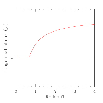
Figure 6: Theoretical relation between tangential shear and source redshift for a lens at $z=0.63$. The vertical axis is in arbitrary units and depends on lens mass.

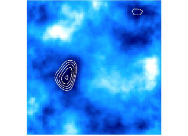
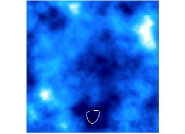
Figure 7: Mass (left) and randomized (right) maps for subfield F4p21. There are approximately $20$K objects in this $35^{\prime}\times 35^{\prime}$ region, or $\sim 16$ per square arc min. North is Up, East is to the Left.

The first shear-selected cluster with tomography analysis was presented in a paper by Wittman et al. 2001 in a pilot project for the DLS. The DLS, covering $\sim$ 50 times more area, should yield a significant sample. In Wittman et al. 2003 the DLS team presents the first shear-selected cluster from the DLS data, with tomography analysis. Figure 7 shows the detection of the cluster in a mass map. The tomography is shown in Figure 8: the left panel presents the mean tangential shear for independent redshift bins; and the right panel indicates the lens (cluster) redshift probability distribution. The best-fit lens redshift is $0.75\pm 0.46$, and spectroscopic observations have confirmed it to be a massive ($\sigma_{v}=980$ km s^-1) galaxy cluster at $z=0.68$. Figure 9 shows a $4^{\prime}\times 4^{\prime}$ image of the cluster.

Figure 8: Left: Tangential shear, around the mass peak, as a function of source photometric redshift. The dotted curve shows the best-fit lens fixed at the spectroscopic redshift of 0.68, and the dashed curve shows the best fit when the lens redshift is allowed to vary ($z=0.55$). Right: Lens redshift probability distribution. The peak is at $z=0.55$ and the rms is 0.15.

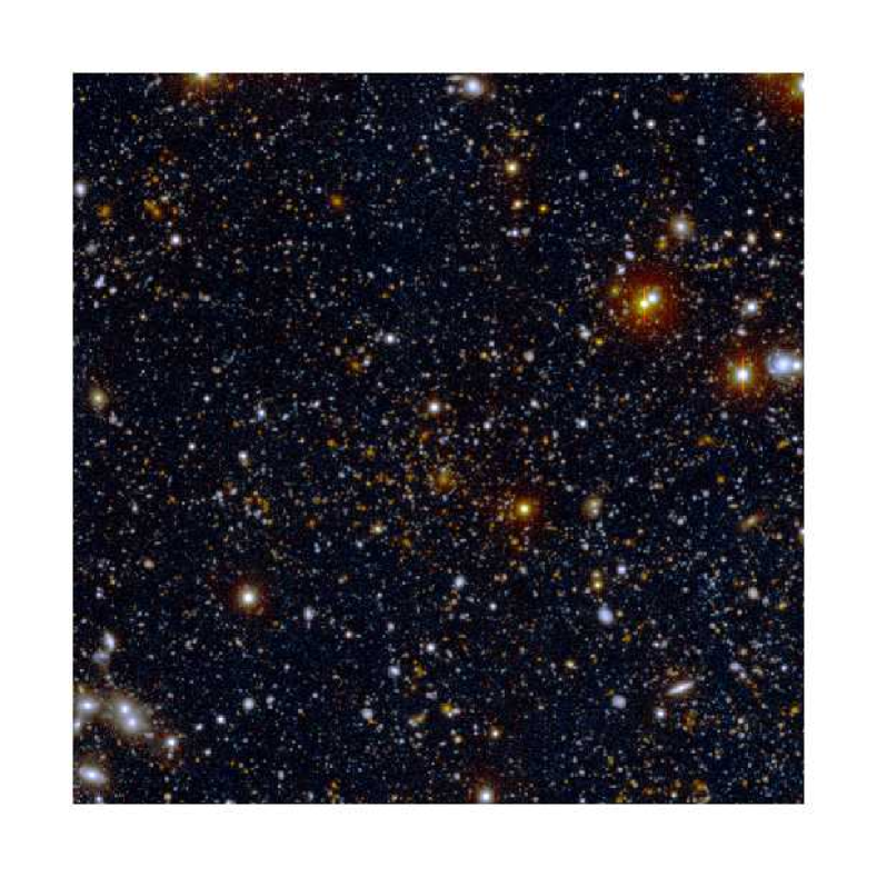
Figure 9: A 4^′ square section of the $R$ image, centered on the BCG. The BCG is $R=20.6$, and the faintest galaxies visible in this reproduction are $R\sim 26$. North is up, and east to the left.

6 Future Work

A preliminary sample of 8 clusters detected in the DLS is being observed with Chandra and 4 more are scheduled to be observed with XMM  (PI. Prof. John P. Hughes). The X-ray data will allow us to quantify the degree to which baryonic matter traces the dark matter distribution. The DLS provides a unique sample of clusters whose selection is unaffected by the distribution of baryons in the cluster, and with this sample we are finding provocative indications that the mass and gas distributions exhibit pronounced differences. Figure 10 shows a DLS potential map for Abell 781, and the X-ray emission in the same region. Clear evidence for differences in the spatial distributions of baryonic and non-baryonic content are observed.

We have also applied for HST time to obtain higher resolution mass maps for a few of these clusters (PI Dr. Anthony Gonzales). The ACS observations will allow us to construct higher resolution mass/potential maps for this clusters ($\sim$50 $h^{-1}$ kpc compared to 400 $h^{-1}$ kpc resolution for the DLS data). With mass maps of such resolution, we will measure the cross-correlation of mass and light on scales of 0.05-1.5 $h^{-1}$ Mpc and will also quantify the radial dependence of the bias, which is of critical importance for derivations of the total cluster baryon fraction.

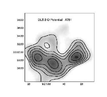
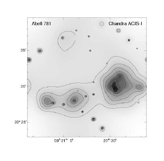
Figure 10: Maps of the gravitational potential (left) and Chandra X-ray emission (right) for Abell 781. Note the difference in the distributions shown in the two maps. While the X-ray emission is predominantly concentrated in the rightmost peak, the potential map shows that a significant fraction of the mass is contained in the lefthand structures.

7 Conclusions

The DLS team has already shown that shear-selection is effective at finding galaxy clusters (Wittman et al. 2001, Wittman et al. 2003). In addition to detecting the shear, the multiband imaging produces photometric redshifts for the clusters. Indeed, combining shear measures with photometric redshift estimates for the background galaxies, one can obtain a redshift estimate for the lens independently of the luminous output of the cluster. This opens the way for construction of a completely baryon-independent cluster sample from the DLS.

8 Acknowledgements

We thank the KPNO and CTIO staffs for their invaluable assistance. NOAO is operated by the Association of Universities for Research in Astronomy (AURA), Inc. under cooperative agreement with the National Science Foundation.

References

- [1] Bernstein, G. M. & Jarvis, M. 2002, AJ, 123, 583
- [2] Birkinshaw, M. 2003, Carnegie Observatories Astrophysics Series, Vol. 3: Clusters of Galaxies: Probes of Cosmological Structure and Galaxy Evolution , ed. J. S. Mulchaey, A. Dressler, and A. Oemler (Cambridge: Cambridge Univ. Press)
- [3] Bolzonella, M., Miralles, J.-M., & Pelló, R. 2000, A&A, 363, 476
- [4] Bruzual, G. A., & Charlot, S. 1993, ApJ, 405, 538
- [5] Cohen, J. G., Hogg, D. W., Blandford, R., Cowie, L. L., Hu, E., Songaila, A., Shopbell, P., & Richberg, K. 2000, ApJ, 538, 29
- [6] Cohen, J. G., Hogg, D. W., Pahre, M. A., Blandford, R., Shopbell, P. L., & Richberg, K. 1999, ApJS, 120, 171
- [7] Coleman, G. D., Wu, C-C., & Weedman, D. W. 1980, ApJS, 43, 393
- [8] Fontana, A., D’Odorico, S., Poli, F., Giallongo, E., Arnouts, S., Cristiani, S., Moorwood, A., & Saracco, P. 2000, AJ, 120, 2206
- [9] Margoniner, V. E., & DLS collaboration 2003, Carnegie Observatories Astrophysics Series, Vol. 3: Clusters of Galaxies: Probes of Cosmological Structure and Galaxy Evolution , ed. J. S. Mulchaey, A. Dressler, and A. Oemler (Pasadena: Carnegie Observatories, http://www.ociw.edu/ociw/symposia/series/symposium3/proceedings.html)
- [10] Peebles, P.J.E., 1980. The Large Scale Structure of the Universe. Princeton: Princeton Univ. Press
- [11] Romer, K. 2003, Carnegie Observatories Astrophysics Series, Vol. 3: Clusters of Galaxies: Probes of Cosmological Structure and Galaxy Evolution , ed. J. S. Mulchaey, A. Dressler, and A. Oemler (Pasadena: Carnegie Observatories, http://www.ociw.edu/ociw/symposia/series/symposium3/proceedings.html)
- [12] Tyson, J. A., Valdes, F., & Wenk, R. A. 1990, ApJ, 349, 1
- [13] Wittman, D., Tyson, J. A., Margoniner, V. E., Cohen, J. G. & Dell’Antonio, I. 2001, ApJ, 557, L89
- [14] Wittman, D., Margoniner, V. E., Tyson, J. A., Cohen, J. G., Dell’Antonio, I. & Becker, A. C. 2003, ApJ, submitted, astro-ph/0210120
- [15] Zwicky, F. 1937, ApJ, 86, 217.