2D MHD modelling of compressible and heated coronal loops obtained via nonlinear separation of variables and compared to TRACE and SoHO observations

An analytical MHD model of coronal loops with compressible flows and including heating is compared to observational data. The model is constructed via a systematic nonlinear separation of the variables method used to calculate several classes of exact MHD equilibria in Cartesian geometry and uniform gravity. By choosing a particularly versatile solution class with a large parameter space we are able to calculate models whose loop length, shape, plasma density, temperature and velocity profiles are fitted to loops observed with TRACE, SoHO/CDS and SoHO/SUMER. Synthetic emission profiles are also calculated and fitted to the observed emission patterns. An analytical discussion is given of the two-dimenional balance of the Lorentz force and the gas pressure gradient, gravity and inertial forces acting along and across the loop. These models are the first to include a fully consistent description of the magnetic field, 2D geometry, plasma density and temperature, flow velocity and thermodynamics of loops. The consistently calculated heating profiles which are largely dominated by radiative losses are influenced by the flow and are asymmetrical being concentrated at the upflow footpoint.

1 Introduction

A significant proportion of the energy emission from the solar corona is concentrated along loops which are believed to trace closed lines of force of the magnetic field, which penetrates the photosphere from below and expands to fill the whole of the coronal volume above an active region (Bray et al., 1991). A coronal loop is therefore an important localised structure which connects the photosphere to the corona through the transition region and may thus be studied to gain information about the heating of the corona as a whole (Aschwanden, 2003).

Early results from the Skylab mission emphasising that the solar corona is not a homogeneous medium but filled with loop structures stimulated much interest in modelling those loop structures. The first models were one-dimensional hydrostatic models which balanced heat conduction and radiative losses with an imposed heating function. Rosner et al. (1978) balanced radiative losses and heat conduction against heating assuming zero heat conduction across the foot points, a restriction relaxed by Hood & Priest (1979) while they neglected radiative losses. Vesecky et al. (1979), Serio et al. (1981) and Wragg & Priest (1981, 1982) added the effects of varying pressure and gravity to their models, as well as the effects of a variable loop cross-sectional area. Cargill & Priest (1980) were the first to add adiabatic plasma flows and concentrated on examining the relationship between cross-sectional area and flow velocity along the loops, while later (1982) introduced non-adiabatic flows balancing the net heat in/out against conduction and radiation with a heating function proportional to the density. Further important hydrodynamic modelling of plasma flows in solar atmospheric structures has been carried out and applied to photospheric flux tubes by Thomas and others, work summarised in Thomas (1996).

A similarly strong interest in loop modelling in recent years has been motivated by the higher resolution results from the Yohkoh, SoHO and TRACE spacecrafts. A systematic study of a one-dimensional hydrodynamic solution class of loops with constant cross-section has been carried out by Orlando et al. (1995a,b), with non-adiabatic flows and balancing the net heat in/out against conduction, radiation and a heating function. Much attention has focused on the form of the heating function as a means of inferring the coronal heating mechanism. Priest et al. (1998, 2000) concluded that their loop model fitted to Yohkoh data yielded higher heating at the apex, although re-analysis of this Yohkoh loop by Mackay et al. (2000) and Aschwanden (2001) concluded that the loop was heated at the foot points. Aschwanden et al. (2001) systematically explored a class of one-dimensional hydrostatic solutions with a non-uniform heating function in exponential form and fitted them to a large sample of EUV loops observed with TRACE. They found that most of the sample of loops could not be modelled by their hydrostatic solution class, and that those which could were heated near the foot points. In the present paper we use a different approach. We do not impose a priori a specific form for the heating function, but instead we calculate it after completing a fitted dynamical MHD model. Hence we calculate a model for the observable quantities first and then find a consistent heating function from the first law of thermodynamics.

Of course some loops in the solar atmosphere are far from equilibrium and time-dependent hydrodynamical loop models have also been developed by e.g. Mariska & Boris (1983), Cargill (1994), Cargill & Klimchuk (1997), Walsh et al. (1995, 1996), Walsh & Galtier (2000), Peres (2000), Reale et al. (2000a, b). In this paper we restrict our modelling and observations to steady-state loops.

To date all heated loop studies have included only one-dimensional hydrostatic or hydrodynamic models. However, in the highly magnetised and sparse coronal plasma the magnetic field is likely to have a significant direct effect on the statics or dynamics of such a curved structure as a coronal loop, while plasma flow, even at such sub-Alfvénic velocities as $20$ km/s (Dara et al., 2002), may have an effect on the heating balance. Moreover, the geometrical details may have an impact on the energy profile of the loop, via the potential energy, and therefore on the heating model. The models in this paper include two-dimensional geometry, compressible MHD plasma flow in uniform gravity and heating in single consistent exact solutions and thereby give a first opportunity to investigate these effects. We fit the geometrical and dynamical aspects of the model to a loop observed by TRACE, a case observed with SoHO/CDS (Schmelz et al. ,2001) and a loop observed by SoHO/SUMER. We also give a model of the energy balance of each loop, including the loop heating.

The paper is organised as follows. The solution class is described in Sect. 2.2, and the method of constructing the models is explained in Sect. 2.3. The observations and data analysis is described in Sect. 3 and models fitted to data sets are presented in Sect. 4. The paper is concluded with Sect. 5.

2 The analytical model

In this section, after an introduction of the basic equations needed in order to establish notation, we proceed to a brief presentation of the key assumptions for the derivation of the particular solution class and an outline of the method employed for the construction of the particular solutions.

2.1 Basic equations

Our model utilize solutions obtained by using a systematic nonlinear separation of the variables construction method in two dimensions and Cartesian geometry (Petrie et al.  2002, henceforth, Paper 1), already seen in spherical geometry (Vlahakis & Tsinganos, 1998). The general analysis of Paper 1 contains the solution class applied here, as well as the prominence and loop models by Kippenhahn & Schlüter (1957), Hood & Anzer (1990), Tsinganos et al. (1993) and Del Zanna & Hood (1996). Basically, in this method and under certain assumptions, the full MHD equations can be reduced to a system of ordinary differential equations (ODE’s) which can be integrated by standard methods.

The dynamics of flows in solar coronal loops may be described to zeroth order by the well known set of steady ($\partial/\partial t=0$) ideal hydromagnetic equations:

$$\rho\left({\bf V}\cdot{\bf\nabla}\right){\bf V}=\frac{1}{4\pi}{\left({\bf\nabla}\times{\bf B}\right)\times{\bf B}}-{\bf\nabla}P-\rho g\hat{Z}\,,$$ (1)

$$\bf{\nabla}\cdot{\bf B}=0\,,\quad\bf{\nabla}\cdot\left(\rho{\bf V}\right)=0\,,\quad\bf{\nabla}\times\left({\bf V}\times{\bf B}\right)=0\,,$$ (2)

where ${\bf B}$, ${\bf V}$, $-g\hat{Z}$ denote the magnetic, velocity and (uniform) external gravity fields while $\rho$ and $P$ are the gas density and pressure. The energetics of the flow on the other hand is governed by the first law of thermodynamics :

$$q=\rho{\bf V}\cdot\left[{\bf\nabla}e+P{\bf\nabla}\frac{1}{\rho}\right]=\rho{\bf V}\cdot\left[\bf{\nabla}h-\frac{1}{\rho}\bf{\nabla}P\right]\,,$$ (3)

where $q$ is the net volumetric rate of some energy input/output, $\Gamma=c_{p}/c_{v}$ with $c_{p}$ and $c_{v}$ the specific heats for an ideal gas, and

$$e=\frac{1}{\Gamma-1}\frac{P}{\rho}$$ (4)

the internal energy per unit mass, with $h=\Gamma e$ the corresponding enthalpy function.

At present, a fully three-dimensional MHD equilibrium modelling with compressible flows is not amenable to analytical treatment and so we assume translational symmetry. Thus, we assume that in Cartesian coordinates $(Z,X,Y)$, the coordinate $Y$ is ignorable ($\partial/\partial Y=0$) and the magnetic and flow fields are confined to the $Z$ - $X$ plane. We model the profile of the loop in the $x$-$z$ plane and ignore variations in the $y$-direction, i.e., we assume that the physics of the $x$-$z$ plane is independent of what happens across the loop in the $y$-direction. All previous equilibrium models of coronal loops mentioned above have been one-dimensional and non-magnetic. To begin with, we represent $\bf B$ by using a magnetic flux function (per unit length in the $\hat{Y}$ direction)

$${\@vec{B}}=\@vec{\nabla}A(Z,X)\times\hat{Y}.$$ (5)

Then, there exist free integrals of $A$ including the ratio of the mass and magnetic fluxes on the poloidal plane (Z-X), $\Psi_{A}(A)$,

$${\@vec{V}}={{\Psi}_{A}\over 4\pi\rho}{\@vec{B}}\,,$$ (6)

where the stream function $\Psi$ is a function of the magnetic flux function $A$ and ${\Psi}_{A}$ is its derivative (Tsinganos, 1982). The component of Eq. (1) along the field may be written as

$$\rho{\bf V}\cdot\nabla I=0,$$ (7)

where

$$I=I(A)=\frac{V^{2}}{2}+gz+\int_{s_{0}}^{s}\frac{1}{\rho}\frac{\partial P}{\partial s}ds$$ (8)

is the generalised classical Bernoulli integral, a further integral of the flow. Eqs. (3,7) may be added to describe the momentum balance

$$q=\rho{\bf V}\cdot\nabla E\,,$$ (9)

in terms of $E$, the total energy of the flow

$$E=\frac{V^{2}}{2}+gz+h.$$ (10)

In general, because of the heat source $q$, the total energy is not conserved along the loop (Sauty & Tsinganos, 1994). Even in the polytropic case where the pressure takes the special form $P=Q(A)\rho^{\gamma}$ the net volumetric rate of energy in/out

$$q=\frac{\gamma-\Gamma}{\Gamma-1}\frac{P}{\rho}{\bf V}\cdot\nabla\rho$$ (11)

is not generally zero (Tsinganos et al., 1992). Only in the special polytropic case with $\Gamma=\gamma$ is the flow adiabatic, and the total energy coincides with the generalised Bernoulli integral and is conserved. However, the general non-polytropic case is the case of interest in this paper.

In the general case, the system of equations (1) - (2) should be solved simultaneously with a detailed energy balance equation in order to yield a self-consistent calculation of the equilibrium values of $\rho$, $P$, $\bf V$ and $\bf B$ along the loop. However, it is a fact that the detailed forms of the several heating/cooling mechanisms in the energy equation are not known, e.g., we do not know the exact expression of the heating along coronal loops which contributes, among others, to the various parts of the net volumetric heating rate q in Eq. (3). Hence, a compromising strategy is to use, for example, a polytropic equation of state and then solve for the values of $\rho$, $P$, $\bf V$ and $\bf B$. Then, we may determine the volumetric rate of net heating from Eq.(3). In such a treatment the heating sources which produce some specific solution are not known a priori; instead, they can be determined only a posteriori. In this paper we shall follow a similar approach.

2.2 The solution class

In order to proceed to the analytical construction of some classes of exact solutions for coronal loops, we make two key assumptions:

1. that the Alfvén number $M$ is solely a function of the dimensionless horizontal distance $x=X/Z_{0}$, i.e.,

   $$M^{2}=\frac{4\pi\rho V^{2}}{B^{2}}=\frac{\Psi_{A}^{2}}{4\pi\rho}=M^{2}(x)\,,$$ (12)

   and

2. that the velocity and magnetic fields have an exponential dependence on $z=Z/Z_{0}$,

   $$A=Z_{0}B_{0}{\cal A}\left(\alpha\right)\,,\qquad\alpha=G(x)\exp{(-z)}\,,$$ (13)

for some function $G(x)$, where $Z_{0}$ and $B_{0}$ are constants. With this formulation the magnetic field has the form

$${\@vec{B}}=B_{0}\alpha{\cal A}^{{}^{\prime}}(\alpha)\left[\hat{X}+F(x)\hat{Z}\right]\,,$$ (14)

where

$$F(x)=\frac{1}{G(x)}\frac{dG(x)}{dx}=\left(\frac{dZ}{dX}\right)_{A}$$ (15)

is the slope of the field line. This is the analogue in Cartesian geometry of the ”expansion factor” in the related wind models in spherical geometry (see Sauty & Tsinganos, 1994). The function $G(x)$ also has a physical meaning. Either by integrating Eq. (15) or by inverting Eq. (13) the equation for the field line defined by $\alpha=\alpha_{0}$ is found to be

$$z=\log G(x)-\log\alpha_{0}.$$ (16)

This is the Cartesian analogue of the cylindrical distance of a field line from the polar axis in spherical wind theory (see Sauty & Tsinganos, 1994). With these assumptions, the momentum-balance equation may be broken down into a system of first-order ODE’s for functions of $x$, and a corresponding system of ODE’s for corresponding functions of the magnetic flux function. The methods of obtaining these ODE’s are described in Paper 1, where all existing solutions are summarised in Table 1 therein.

The solutions used in this paper are taken from the first family in Table 1 in Paper 1. In the remaining of this section we examine the general case, with all constants non-zero. The corresponding expressions for the magnetic flux function $A$, the mass flux per unit magnetic flux $\Psi_{A}$, the density $\rho$, the magnetic induction $\bf B$ and the velocity $\bf V$ are (see Paper 1)

$$A(\alpha) = Z_{0}B_{0}\int\sqrt{2C_{1}+\lambda C_{2}\alpha^{\lambda-2}}d\alpha,$$ (17)

$$\Psi_{A}(\alpha) = \frac{B_{0}}{\sqrt{gZ_{0}}}\sqrt{2D_{1}\alpha^{2}+\lambda D_{2}\alpha^{\lambda}},$$ (18)

$$\rho(x,\alpha) = \frac{B_{0}^{2}}{4\pi gZ_{0}}\frac{2D_{1}\alpha^{2}+\lambda D_{2}\alpha^{\lambda}}{M^{2}},$$ (19)

$$P(x,\alpha) = \frac{B_{0}^{2}}{4\pi}\left[P_{0}+P_{1}(x)\alpha^{2}+P_{2}(x)\alpha^{\lambda}\right],$$ (20)

$${\@vec{B}} = B_{0}\sqrt{2C_{1}\alpha^{2}+\lambda C_{2}\alpha^{\lambda}}\left[\hat{X}+F(x)\hat{Z}\right],$$ (21)

$${\@vec{V}} = \sqrt{gZ_{0}}\sqrt{\frac{2C_{1}\alpha^{2}+\lambda C_{2}\alpha^{\lambda}}{2D_{1}\alpha^{2}+\lambda D_{2}\alpha^{\lambda}}}M^{2}\left[\hat{X}+F(x)\hat{Z}\right].$$ (22)

where $C_{1}$, $C_{2}$, $D_{1}$, $D_{2}$ and $\lambda$ are constants. Note that we may choose the constants such that $B_{0}$ is the component of the magnetic field at a reference point. Also note that the general non-polytropic case has two “scales”: $Z_{0}$ and $2Z_{0}/\lambda$. In the expression for the pressure $P_{0}=f_{0}=$ constant, while $P_{1}$ and $P_{2}$ satisfy the following ODE’s

$$P_{1} = C_{1}\left[FM^{2^{\prime}}-F^{{}^{\prime}}(1-M^{2})-F^{2}-1\right]+\frac{D_{1}}{M^{2}}\,,$$

$$P_{2} = C_{2}\left[FM^{2^{\prime}}-F^{{}^{\prime}}(1-M^{2})-\frac{\lambda}{2}(F^{2}+1)\right]+\frac{D_{2}}{M^{2}}\,.$$

Using the above definitions for the pressure “components” together with the ODE’s from Table 1 in Paper 1, we calculate that for the general case we have the following final system of equations for the unknown functions of $x$, including the slope of the field lines $F$ :

$$\frac{d\ln G}{dx} = F\,,$$ (23)

$$M^{2^{\prime}}(x) = \frac{\mathcal{C}\lambda F/M^{2}-2F(F^{2}+1+P_{1}/C_{1})}{\mathcal{C}/M^{4}+2}\,,\ \mbox{where}\ \ \mathcal{C}=\frac{D_{2}/C_{2}-D_{1}/C_{1}}{1-\lambda/2}\,,$$ (24)

$$F^{\prime}(x) = \frac{FM^{2^{\prime}}-F^{2}-1+D_{1}/C_{1}M^{2}-P_{1}/C_{1}}{1-M^{2}}\,,$$ (25)

$$P_{1}^{\prime} = -\frac{2D_{1}F}{M^{2}}-2C_{1}(1+F^{2})M^{2^{\prime}}-2M^{2}FF^{\prime}\,.$$ (26)

$$P_{2}(x) = C_{2}\left(FM^{2^{\prime}}-F^{\prime}(1-M^{2})-\frac{\lambda}{2}(1+F^{2})\right)+\frac{D_{2}}{M^{2}}\,,$$ (27)

Finally, consider the energy balance along the loop; the net volumetric rate of heating input/output $q$, equals to the sum of the net radiation $L_{R}$, the heat conduction energy $\nabla\cdot{\bf F}_{C}$, where ${\bf F}_{C}$ is the heat flux due to conduction, and the (unknown) remaining heating $E_{H}$,

$$q=E_{H}+L_{R}-\nabla\cdot{\bf F}_{C}.$$ (28)

The net heat in/out $q$ is calculated from the MHD model using the first law of thermodynamics Eq. (3), while the radiative losses from the optically thin plasma $L_{R}$ are described by the equation

$$L_{R}=-(n/2)^{2}Q(T),$$ (29)

(Raymond & Smith, 1977) with standard solar atmospheric abundances as in Rosner et al. (1978), where $n$ is the particle number density (we assume that the plasma is fully ionised) and $Q(T)$ is a piecewise function of $T$ described in Rosner et al. (1978). The thermal conduction energy is calculated assuming that conduction is mainly along the field, using the expression

$$-\nabla\cdot{\bf F}_{C}=\frac{\partial}{\partial s}\left(\kappa_{\small||}\frac{\partial T}{\partial s}\right)-\frac{\kappa_{\small||}}{B}\frac{\partial B}{\partial s}\frac{\partial T}{\partial s},$$ (30)

(Spitzer, 1962) where subscripts $||$ indicate values and derivatives along the field line, and the variation of the magnetic field strength along the field line is taken into account (Priest, 1982, p86).

We present the physical parameters of each loop as functions of arc length $s$. The arc-length along a loop is given by

$$ds^{2}=dx^{2}+dz^{2}=(1+F(x)^{2})dx^{2}$$ (31)

and the $(x,\alpha)$-dependent physical parameters of a loop can be understood as functions along the loop by holding $\alpha$ constant (the definition of a field line since $\alpha$ is a flux function) and integrating Eq. (31) for $s$ from the left foot point to the right foot point.

2.3 Construction of solutions

We generate loop-like solutions as follows. We begin by calculating the right half of the loop, beginning from the loop apex at $x=0$. The symmetry properties of Eqs. (23 - 27) ensure that on integrating from $x=0$ in the negative direction the other half of a symmetric loop-like solution is obtained. In the sub-Alfvénic case the equations have no critical points and can be integrated without difficulty. In the trans-Alfvénic case a shooting algorithm is required to integrate through the critical Alfvén point (Vlahakis & Tsinganos, 1998; Paper 1) but since steady super-Alfvénic flows have not been observed in the solar atmosphere we will concentrate on sub-Alfvénic examples here. In this paper we use a similar shooting algorithm to fix the foot point separation of each sub-Alfvénic loop. The solution class allows us to fix all physical quantities at the apex: the height, magnetic field strength, velocity, density and temperature. Having chosen values for these quantities at the apex we begin the integration. As the solution approaches the solar surface at $z=0$ it will be clear whether the foot point separation is greater or less than the desired (observed) value and a remaining free parameter can be adjusted accordingly. This process is repeated until the solution is fitted to the desired (observed) configuration.

In this paper we present models fitted to data, where available, in five ways: we fit the loop height and foot point separation as described above, the plasma density and temperature, the line-of-sight velocity or velocities of proper motions whose components perpendicular to the line of sight can be measured, and we forward-fit synthetic emission models to observed emission patterns.

It can be seen from the equation for a magnetic field line, Eq. (16), that two field lines defined by $\alpha=\alpha_{1}$ and $\alpha=\alpha_{2}$ differ from each other only by a vertical translation, and that for any point $(Z_{1},X)$ on the first field line, the corresponding point on the second field line $(Z_{2},X)$ can be found from it by moving vertically a distance

$$Z_{2}-Z_{1}=\log{\frac{\alpha_{1}}{\alpha_{2}}}.$$ (32)

We may model the cross-sectional width of a loop by taking two such field lines and by considering the area between these lines to constitute the loop model. Then the loop necessarily has maximum cross-sectional width at the apex, the remainder of the width profile being uniquely defined by the geometry of a field line. Thus the loop width $W$ is not a free function to be imposed as in one-dimensional studies, e.g., Cargill & Priest (1982); Aschwanden & Schrijver (2002), but is related to the slope of the loop $F$ by

$$W(s)=\left.\log{\frac{\alpha_{1}}{\alpha_{2}}}\right/\sqrt{1+F^{2}}.$$ (33)

If a loop is observed to be tilted with respect to the vertical direction then we may still model the loop in the $x$-$z$ plane by tilting our coordinate system accordingly. We must take into account the effect of this tilt on the physics of the loop. The gravitational force acts at an angle to the $z$-axis and the loop cuts through the stratified atmosphere at an angle. Therefore in the model the gravitational force must be multiplied by the cosine of the angle of tilt and vertical scale heights must be divided by this cosine.

It is well-known that plasma flow is generally present in loops (e.g. Dara et al., 2002). However, only limited information about the magnitude of the loop plasma velocities is available today from satellite data: line-of-sight measurements from dopplergrams in the case of the CDS and SUMER data sets, and high-resolution movie measurements of velocities of inhomogeneities, or proper motions, in the plasma flow in the case of the TRACE example. We model these measurements by taking the two-dimensional velocity field from our MHD solution and, taking the geometry of the loop and the viewing angles of the instrument relative to the loop into account, we calculate model line-of-sight and perpendicular velocity components to be compared to the observations. Thus, taking the planar loop to be confined to the $x$-$z$ plane and centred at the origin, we define by $\theta$ the angle in the $x$-$y$ plane between the $x$ axis and the line from the origin to the instrument, and by $\phi$ the angle between the line from the origin to the instrument and the plane $z=0$. Then, assuming that the distance from the instrument to the loop is much larger than the size of the loop, the line-of-sight velocity $V_{LOS}$ as observed by the instrument and the velocities in the two directions of the image perpendicular to the line of sight, $V_{\perp x}$ and $V_{\perp y}$, are given by

$$\left(\begin{array}[]{c}V_{\perp x}\\ V_{\perp y}\\ V_{LOS}\end{array}\right)=\left(\begin{array}[]{ccc}\cos\theta\cos\phi&\sin\theta\cos\phi&-\sin\phi\\ -\sin\theta&\cos\theta&0\\ \cos\theta\sin\phi&\sin\theta\sin\phi&-\cos\phi\end{array}\right)\left(\begin{array}[]{c}V_{x}\\ V_{y}=0\\ V_{z}\end{array}\right).$$

The velocity perpendicular to the line-of-sight has magnitude $V_{\perp}=\sqrt{V_{\perp x}^{2}+V_{\perp y}^{2}}$, so that $V^{2}=V_{\perp}^{2}+V_{LOS}^{2}$.

3 Observations, data reduction and loop diagnostics

There is some controversy surrounding the issue of extracting measurements of coronal densities and temperatures from emission data. Judge & McIntosh (1999) contrast the probable multi-thermal nature of loops consisting of strands with inefficient cross-field thermal conduction (Litwin & Rosner, 1993) with the evidence from TRACE that loops in significantly different temperature filters are never co-spatial, and stress the ill-posedness and non-uniqueness of inverse modelling techniques applied to the transition region and corona. In this work, densities and temperatures have been calculated for the TRACE example using the the narrowband 171 Å  and 195 Å  two-filter fluxes (e.g., Aschwanden et al. 2000; Winebarger et al. 2002). Forward-fitting of our model to two-filter fluxes, $F_{171}(s)$ and $F_{195}(s)$, does not suffer from the ambiguity of filter-ratio temperature fits, $R=F_{195}/F_{171}$, which has been shown to have, besides the $T\approx 1.0$ MK solution, also a high-temperature solution at $T\approx 5.0$ MK (Testa et al. 2002). But Winebarger et al. (2002) demonstrated that the $T=5.0$ MK solution of Testa et al. (2002) is generally not consistent with combined TRACE and Yohkoh/SXT data, and similarly, Chae et al. (2002) demonstrated that the $T=5.0$ MK solution is not consistent with TRACE triple-filter data. An additional confusion in the temperature analysis of multi-filter data was raised by Schmelz et al. (2001), who showed that the emission measure distribution of a loop structure observed with CDS over a temperature range of $\log T=5.4-6.4$ displays a rather broad temperature distribution with the mean temperature increasing towards the loop top, and thus concluded that the analysed CDS loop structure has at every location a broad temperature distribution and heating occurs at the loop top. Martens et al. (2002) characterised the smoothed DEM of Schmelz et al. (2001) as a flat plateau and pointed out that any filter-ratio method is inaequate to determine the temperature of such a loop system (see also Schmelz, 2002). However, the CDS observations of Schmelz et al. (2001) can easily be understood if the following facts are taken into account: (1) The effective spatial resolution of CDS is $\approx 10"-15"$, compared with $\approx 1"$ of TRACE, (2) TRACE 171 Å  images reveal for every loop structure observed with CDS at $T\approx 1.0$ MK at least $\approx 10$ loop threads, (3) the broad DEM distribution of a CDS loop structure is not smooth but consists of multiple temperature peaks which clearly indicate multiple loop threads with different temperatures (Aschwanden 2002), (4) the centroid position of the CDS loop structure was found to exhibit displacements in each CDS temperature filter (as presented by Trae Winter at the ”Coronal Loop Workshop” in Paris, November 2002), which confirms that the CDS loop structure consists of multiple, non-cospatial loop threads, and (5) the combined emission measure distribution of many loop threads over a broad a temperature range bears a hydrostatic temperature bias that yields an average temperature increasing with height (Aschwanden & Nitta 2000). From these facts there is clear evidence that a loop structure seen by CDS consists of multiple loop threads with different spatial positions and different temperatures although Martens et al. (2002) argue that, because the high-temperature edge as well as the low-temperature edge of their DEM plateau moves towards higher temperatures approaching the loop top, high temperatures must exist near the loop top which are not found lower down the structure, and so individual loop strands are unlikely to be exactly isothermal. Of these loop threads, TRACE resolves a subset that coincides in the temperature sensitivity range of a TRACE narrow-band filter. It is therefore imperative to apply a model only to a resolved loop thread, rather than to a multi-temperature bundle of loop threads that make up a CDS loop structure. Since we analyse the same loop structure as described in Schmelz et al. (2001), we apply our MHD model only to a single CDS temperature filter (Mg ix 368 Å,1 MK), being aware that even the loop structure seen in this single filter still consists of multiple threads, given the poor CDS resolution, and thus expect only to extract average density and velocity parameters for this loop system at the given temperature range of the Mg ix filter ($T=1$ MK). Also, we apply a forward-fitting technique to the observed emission, as recommended by Judge & McIntosh (1999), to avoid the ill-posedness of filter-ratio techniques. In the three cases we model here, we use in our forward-modeling only a single image (CDS, SUMER) or an image pair of similar temperature (TRACE) to avoid confusion between loop strands of different temperatures.

We use observations from TRACE in the 195 Åand 171 Å bands taken on 24-26 October 1999, SoHO CDS observations used by Schmelz et al. (2001) taken on 20 April 1998 and SUMER observations from March 25, 1996. The TRACE instrument was pointing on a well-defined isolated loop system at $-426\arcsec,-275\arcsec$ (see Fig. 1, top left picture). The field of view is of $768\times 768$ pixels whereas the pixel size is 0.5″. The corrections that we applied are the following: we subtracted the readout pedestal and the dark current, we cleaned out the pixels damaged due to cosmic-rays and we extracted the CCD readout noise.

In order to derive the geometry of the loop as well as the physical parameters we followed Aschwanden et al. (1999). We used the stereo package (Aschwanden et al., 1999), which is part of the solar software (SSW) in order to reproduce the geometry of the loops. As the lines used are optically thin, when we diagnosed physical parameters such as the electron density, we took great precautions to extract the background emission as in Aschwanden et al. (1999). We supposed that the background around a loop can be derived from a stripe of emission which contains the loop (see Fig. 1, top left picture). Each cross-section of a stripe contains a cross-section intensity profile of the loop as well as non-loop intensity that surrounds it. The intensity ‘outside’  the loop, was interpolated across the loop region in order to simulate the background contribution there. We tried several boundaries of the loop profile and choose those maximising the difference between the total and the background flux, as in Aschwanden et al. (1999). The extraction of the background was performed for the loop as it appears in the Fe ix 171 Å and the Fe xii 195 Å lines. We computed the temperature and the emission measure using the trace_teem routine which applies a filter ratio technique with the Fe ix 171 Å and the Fe xii 195 Å lines. We derived the mean electron density $n_{e}$ at each point along the loops using Eqs. (34),

$$n_{e}\,=\,\sqrt{\frac{EM}{w}}\ ,\ \ \ w=\frac{\int F_{T}(s,t_{j})-F_{B}(s,t_{j})\,dt_{j}}{max(F_{T}(s,t_{j})-F_{B}(s,t_{j}))}$$ (34)

where $w$ is the loop width, $F_{T}(s,t_{j})$ is the total flux at a distance $s$ along the loop and at $t_{j}$ across it, and $F_{B}(s,t_{j})$ is the background flux.

We tried to measure the proper motions, if any, of the loop plasma. We first centered very carefully the 171 Å every 30 sec. images and made a movie with them. Fig. 2 shows frames from this movie of proper motions along the loop. We show a part of the loop in three 171 Å  images close in sequence, showing the displacement of two blobs of material indicated by arrows. The dashed lines in the second and third pannel show the initial positions of the two blobs. We believe that the material is moving - or the excitation is moving - from the left to the right foot point. Since half a pixel is the minimum displacement and it corresponds to a velocity of 17 km/s, we consider this as the error of the measurements. As “points” we select bright features within the loop, which can be followed in at least two images. The various points measured were located in only two images, with the exception of three points which are each found in three images. The measurement is very subjective, but since quite some points are measured, especially near the top, and most of their velocities are within the range of 30-40 km/s we believe that this value is close to the real velocity. The mean velocity that we calculate is of the order of 30 km/sec. We show in the bottom picture of Fig. 2 the evolution of the intensity along another segment of the loop plotted against time. This variation of intensity travelling toward the right footpoint of the loop may be associated with a flow along the loop. We can estimate roughly from this figure a velocity of 40-50 km/sec. It is possible that the observed “proper motions” could also be wave disturbances, propagating with very slow subsonic speed. To distinguish between a flow motion and a wave one test would be: a flow usually has a temperature difference to the pre-existing plasma in the loop, while a wave motion does not change the temperature at all. For these observations we lack 195 Å  images that are close in time to the series of 171 Å  images where we see the motion and so we cannot check the temperature variation at the position of the blobs. However, in the 171 Å images we observe individual blobs that we can follow in up to three images. We do not detect any oscillation of the intensity in this particular loop. This as well as the slow velocities found leads us to conclude that these velocities are associated with plasma flow and not wave motion.

As for the CDS data, we applied the usual CDS procedures to treat the geometrical corrections and to calibrate them. The dopplershifts along the loop, are computed in the Mg ix 368 Å(1 MK) line. For each selected point along the loop, we took the sum of the 4 nearest individual spectral profiles (corresponding to 4 spatial pixels). Thus, for each selected point we applied to that less noisy spectral profile a double gaussian fit to take into account the blend due to the Mg vii line at 367 Å. Before the fitting, we subtracted from each spectral profile a background one, selected from dark regions near the loop. In order to estimate what should be the zero velocity, at the surface of Sun, we selected an area on the Mg sc ix dopplergam, on the disk, but very close to the limb. The wavelength calibration was based on the assumption that the average dopplershift near the limb is very close to zero, as it was suggested from works like the one by Peter & Judge (1999).

The SUMER data we used were obtained during a raster that took place on March 25, 1996. The instrument recorded the Ne viii 770, 780 Å  and the C iv 1548 Å spectral lines. We applied the usual SUMER data reduction and geometrical corrections. We calculated the dopplershifts along the loop following the same method as with CDS. The background spectral profile was also subtracted before the fitting procedure. As we couldn’t use a reference spectrum to calibrate the measured dopplershifts (as it is done in e.g. Teriaca et al., 1999) we selected a quiet Sun area away from the active region and we supposed that there should be a blueshifted of 2 km/s, which is the mean measured dopplershift for that line (Peter, 1999; Dammash et al., 1999).

4 The models

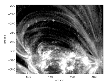
Figure 1: An MHD model of a loop observed by TRACE fitted to observational data: shown are the TRACE image of the loop system with the loop of interest contained within crosses (left picture) and the model field line (solid line) fitted to the observed line, represented by diamonds (right picture) in the $x$-$z$ plane.

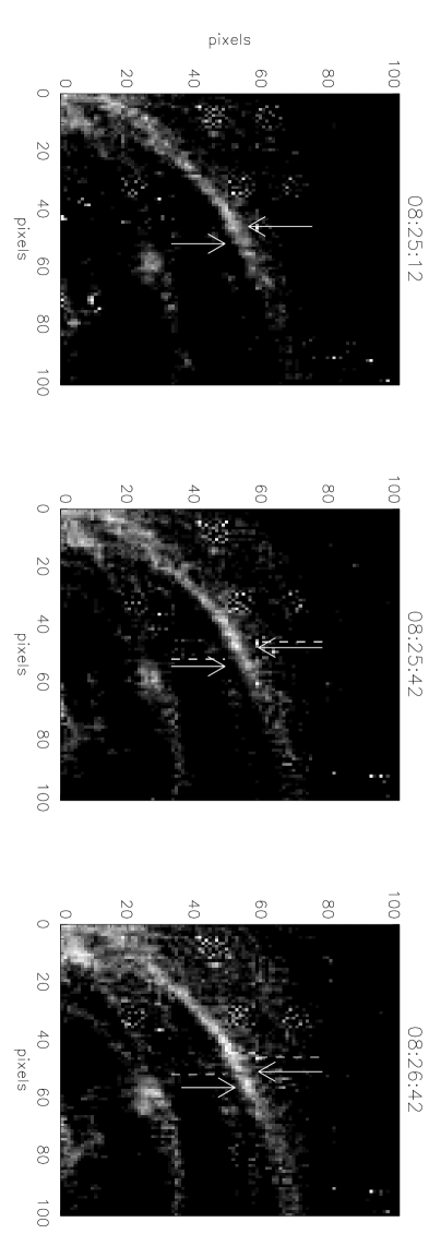
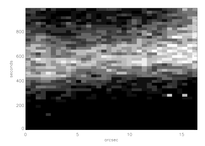
Figure 2: Proper motions along the loop shown in Fig. 1. We show in the top three pictures a part of the loop in three 171 Å images close in sequence, showing the displacement of two blobs of material indicated by arrows. The dashed lines in the second and third pannel show the initial positions of the two blobs. The mean velocity we calculate is of the order of 30 km/sec. We show in the bottom picture the evolution of the intensity along another segment of the loop (horizontal axis) versus time (vertical axis). Black represents unenhanced loop emission and shades of grey represent enhanced emission. This variation of intensity travelling toward the right footpoint of the loop may be associated with a flow along the loop. We can estimate roughly from this figure a velocity of 40-50 km/sec.

We describe in this section details of the three loops as observed and modelled. The models are fitted to the observations in many different ways: by geometry (loop height, foot point separation and, less precisely, loop width), emission measure, density, temperature and velocity. The resulting momentum balance, energy profile and heating profile are then described.

4.1 The observable quantities: loop geometry, emission measure, density, temperature and velocity

Figure 3: An MHD model of a loop observed by TRACE fitted to observational data: shown are (a) the particle number density, (b) the temperature, (c) the flow velocity, (d) the loop width and (e) the 171 Å and (f) the 195 Å emission patterns compared with the synthetic forward-modelled emission from the MHD model. The forward-modelled emission patterns are computed using the TRACE response functions. All are graphed against arc length along the fieldline of the loop shown in Fig. 1. In these plots, the observed values are represented by $x$ symbols and the model by the lines. In the velocity plot the modulus $|{\bf V}|$ is graphed with a dashed line while a simulated perpendicular velocity profile is represented by a dotted line.

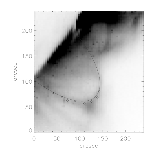
Figure 6: An MHD model of a loop observed with SoHO/CDS (Schmelz et al., 2001), fitted to observational data: the plots are organised as in Fig. 1. The CDS image of the loop is in Si xii 520.66 Å (left picture), and shows the points used for the loop fitting, as well as the fitted loop of the right picture projected onto the image. The fitted field line of the model is shown in the $x$-$z$ plane along with these points (diamonds) for further comparison.

Figs. 1, 6 and 9 show pictures of the image containing each loop and plots of solution field lines fitted to the observed loop shape in the plane of the loop. Figs. 3, 7 and 10 show plots of the density, temperature, together with the absolute and line-of-sight velocities of the models and comparisons of forward-modelled synthetic emission patterns compared to the observed emission. Where available the observed values are also plotted. It must be noted that there are ambiguities in some aspects of the fitting of the models to the data. Coronal magnetic field observations are not sufficiently advanced at present for a detailed model fit and so we impose typical coronal field strengths in our models of $2$-$5$ G at the apex to $50$ - $100$ G, depending on field line geometry and inclination. Although the ODE’s Eqs. (23-27) depend on the magnetic field strength $|{\bf B}|$ via $M$ we find that the value of $|{\bf B}|$ does not significantly affect the physical properties of the fluid. We integrated Eqs.(23-27) with various start values of $|{\bf B}|$ up to a factor of $10$ greater and smaller than those in the examples presented, keeping the start values of the other parameters fixed. The only parts of the model changing significantly are the magnetic forces themselves in Figs. 5, 8 and 11 pictures a-d, while the other plots change very little. An exception to this rule is the case where the magnetic field is too weak for the magnetic forces to be able to balance the other forces as seen in these pictures, in which case the integration simply fails indicating that an equilibrium is not possible. The effect on the system of varying $|{\bf B}|$ can be seen explicitly in Eqs. (23-27). The strong coronal magnetic field combined with the slow flow velocities observed in the corona together cause the flow to be very sub-Alfvenic ($M<<1$). Hence varying $|{\bf B}|$ by a factor of $10$ has little effect on the size of $M$ compared to the other variables, whose sizes are fixed by the observations. It is for this reason that the response of the plasma parameters to such variations in $|{\bf B}|$ is small.

There is some ambiguity in the fitting of the temperature, density and velocity models, as well as the widths, due both to difficulties in measuring quantities along entire loop lengths precisely and to limits in the versatility of the solutions. In the TRACE example Figs. 1, 3 observations of the 171 Å and 195 Å emission and filter ratio calculations of the density and temperature are available along about half of the loop length. Elsewhere the emission is mixed with that of neighbouring loops and so reliable measurements are not possible. A measure of the shape of the entire loop is available (see Fig. 1). The filter ratio measurements describe a near-isothermal loop whose density decreases with height. We are able to fit the density and temperature and emission patterns of this loop reasonably for much of the region where observations are available. In the CDS example, the DEM temperature and density measurements from Schmelz et al. (2001) are multi-thermal while our emission data are extracted from a single Mg IX image. Since the emission data and the density and temperature data are inconsistent with each other our approach is to concentrate on forward-fitting our MHD model to the emission data while using the density and temperature data as a guide, providing information about the density distribution and the temperature magnitude. On fitting the emission model to the observations we find a reasonable fit to the DEM density data, and we find a temperature model which is within the range of the temperature data although more nearly isothermal. More isothermal models or models with flatter density profiles could not be made to fit the observed emission. A fit of T closer to many of the Schmelz et al. (2001) temperature data points at around 2 MK in this example requires a density function larger than the Schmelz et al. (2001) density data, which seems very unlikely since many loops seem to contribute to these density measurements. Besides, the Mg IX line at 1 MK is significantly cooler than 2 MK and so we would expect this image to pick up some of the cooler strands of this loop system. The velocity measurements derive from a dopplergram from this same Mg IX image and, taking the angles of the loop geometry and tilt into account as described in Sect. 2.3, we are able to model these measurements to reasonable accuracy. Filter ratio or DEM measurements of the density and temperature for the SUMER example are not possible, and so density measurements are calculated from a single Ne VIII image using the response function and taking the temperature to be $0.7$ MK. Velocity measurements are also extracted from this same image. While these measurements are more scattered than those of the TRACE and CDS examples, approximate fits of the MHD model to the intensity, density and velocity measurements with a near-isothermal temperature model at around $0.7$ MK are given.

A measure of the width of the loop is made difficult by the mixing of emission with neighbouring loops in all three examples and low resolution of the instruments in the CDS and SUMER examples. Therefore there is much uncertainty in these measurements. Furthermore, because of the self-similar structure of the solution class (see Sect. 2) the profile of the width of a model loop is defined by the shape of the loop so that a solution fitting both the observed field line shape and the observed loop width is not generally possible within our models. The expanding cross-sections derive directly from the self-similar structure of the solutions as described in Sect. 2.3 which for the moment we cannot avoid, since the self-similar assumption embodied by Eqs. (12,13) is crucial for us to solve the MHD equations. The model widths are compared to the observed widths in Figs. 3, 7 and 10.

The flow in our examples is unidirectional from one foot point to the other as in the models by Cargill & Priest (1980, 1982) and Orlando et al. (1995a, 1995b). However, unlike those models the flow in our examples is not sustained by a pressure difference between the loop foot points, the siphon mechanism. This mechanism is included in the models by Cargill & Priest (1980, 1982) and Orlando et al. (1995a, 1995b) because the only force which can initiate in these models a unidirectional loop-aligned flow along the field lines is a suitable pressure gradient. However the physical details of the initiation of flow in the corona are not well known. The flow may not have been initiated in a pre-existing loop, but may have been caused during the loop’s formation by the interaction of several forces. Moreover in the steady state such a pressure difference is not necessary to maintain the flow. A symmetric profile for the plasma inertia (signifying e.g. acceleration up one loop leg and decceleraton down the other, or vice versa) may easily be balanced in a symmetric plasma model by gravity, the pressure gradient and, in two dimensions, by the Lorentz force. Because we are interested in modelling steady states, for simplicity we choose to model symmetric loops which have pressure profiles symmetric over the loop length. Although the flow is unidirectional, we are not describing siphon flows. We remark that the well-known ”siphon flow” models of isolated flux tubes by e.g. Thomas (1988) and Montesinos & Thomas (1989) do not include pressure differences despite their use of the term “siphon flow”.

4.2 Momentum balance

Figure 4: The breakdown of momentum balance along and across a steady coronal loop. Shown are the magnetic pressure gradient $P^{m}$, the magnetic tension force $T$, the gas pressure $P$, the gravitational force $g$ and the inertial force $I$. Also shown are the components of these forces resolved in the direction tangent (normal) to the field, with subscript $s$ ($n$). This diagram corresponds to the example momentum plots in Figs. 5, 8 and 11 as described in the text.

Figure 5: An MHD model of a loop observed by TRACE fitted to observational data: shown are the breakdown of the momentum balance (a) along and (b) across the loop with magnified plots (c, d), (e) the energy integral along the loop and (f) the volumetric energy rate along the loop all graphed against arc length along the loop. In the momentum-along pictures, positive momentum means momentum directed from the left foot point to the right, while in the momentum-across pictures, positive momentum means momentum directed from inside the loop outwards. In the heating plot, the net heat in/out is represented by the dashed line, the radiative losses by the dot-dashed line, the losses due to conduction by the dotted line, and the remaining heating by the thick solid line. Except for a small region near the apex, radiative losses are larger than conductive losses. The heating profile is largely dominated by radiative losses but, influenced by the flow, it is not symmetrical, but is concentrated at the inflow foot point.

Figure 7: An MHD model of a loop observed with SoHO/CDS (Schmelz et al., 2001), fitted to observational data: the plots are organised as in Fig. 3 . The observational data in the density and temperature plots are taken from Table 2 of Schmelz et al. (2001). Because the Si xii emission data from the image in Fig. 6 and the multi-thermal DEM density and temperature data are inconsistent, priority has been given to fitting the emission model, while the density and temperature data are used to guide the modelling (see text). The result is a near-isothermal model. The observational data in the velocity plot were calculated from dopplergrams computed from the same Si xii image in Fig. 6 using Gaussian fitting techniques. Error bars are omitted from the width plot because the errors are too large.

Figure 8: An MHD model of a loop observed with SoHO/CDS (Schmelz et al., 2001), fitted to observational data: the plots are organised as in Fig.5. Note that here, as in Fig. 5, the radiative losses dominate the energy balance, but an asymmetric heating function results because of the influence of the flow.

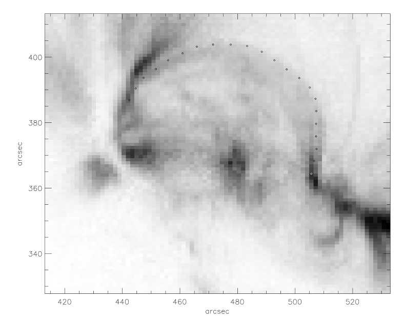
Figure 9: An MHD model of a loop observed by SUMER fitted to observational data: shown are the SUMER image of the loop system with the loop of interest indicated by a dotted line left picture), and the model field line (solid line) fitted to the observed line, represented by diamonds (right picture) in the $x$-$z$ plane.

Figure 10: An MHD model of a loop observed by SUMER fitted to observational data: the plots are organised as in Fig. 1.

Figure 11: An MHD model of the loop observed by SUMER fitted to observational data: the plots are organised as in Fig. 5. Note that in these plots the loop profiles resemble the profiles of the downflow (right) leg of the TRACE and CDS examples in Figs. 5, 8.

Although coronal loops are well known to be magnetic structures, the component of force balance along the loop excludes the Lorentz force, and so it has become common to model them as approximately one-dimensional structures imposing hydrostatic (Rosner et al., 1978; Serio et al., 1981; Aschwanden et al., 2001; Aschwanden & Schrijver, 2002) or steady hydrodynamic (Cargill & Priest 1980, 1982; Orlando et al., 1995a,b) equilibrium along the loop. The inclusion of a second cross-field dimension in our modelling allows the Lorentz force to interact with the other forces across the loop and self-consistently to determine its shape and cross-section. Our models are the first loop models to include these cross-field effects fully and consistently. Given the highly magnetised nature of the solar corona, inclusion of the magnetic field is important in describing the loop dynamics. Of particular importance is the fact that on a curved loop in two dimensions the inertial term is not field-aligned and so the plasma velocity may be greatly influenced by the magnetic field as well as the other forces, unlike the one-dimensional case. Furthermore, in the siphon flow models of Cargill & Priest (1980, 1982) and Orlando et al. (1995a, 1995b) the flow velocity is determined by the density for a given loop cross-sectional area which these authors impose as a free function, while in our models the magnetic field selconsistently imposes the cross-sectional area of the loop, thereby having a further direct influence on the plasma dynamics.

Fig. 4 is an illustration of the breakdown of the momentum balance along and across a coronal loop into the five constituent forces: inertia of the plasma, magnetic tension, magnetic and gas pressure gradients and the gravitational force, as well as components of these forces resolved in directions tangent and normal to the field. This diagram corresponds to the example momentum plots in Figs. 5, 8 and 11 as described later in this subsection. Note that the magnetic forces cancel in the tangential direction because the Lorentz force is perpendicular to the field. In the direction normal to the field, the Lorentz force is non-zero and it is coupled with the remaining forces. The magnetic tension force acts vertically downwards because of the curvature of the loop. The magnetic pressure gradient force has an upward vertical component because of the vertically stratified structure of the magnetic field strength which decreases with height. On the other hand, the magnetic field strength increases with slope because in an active region neighbouring field lines are generally bunched close together near their foot points, generally located at a strong flux source/sink, and their separation increases with distance from the source/sink. Hence, the horizontal magnetic pressure gradient force points towards the interior of the loop. The gas pressure gradient force has an upward vertical component because of the stratification. On the other hand, the horizontal component of the gas pressure gradient force points towards the center of the loop as the corresponding magnetic pressure gradient force does because emission is generally found to be significantly higher in the region of active region loop foot points than close to an apex; in such near-isothermal structures, this implies that the gas pressure is higher at the loop foot points in comparison to the interior of the loop at the same horizontal distance. The normal component of the inertia points inside the loop towards the loop’s centre of curvature, as expected, while the tangential component is non-zero because the loop is not circular and the curvature varies along the loop. In particular, it is negative (i.e., it points towards the footpoints) because the curvature is increasing from the left foot point to its maximum value at the apex. The inertia on the right leg would be a mirror image of this, with a positive tangential component indicating that the curvature is decreasing away from the apex towards the right foot point.

Figs. 5, 8 and 11 show the breakdown of the momentum balance along the field and across the field, the volumetric energy profile along the loop and the volumetric energy rate per unit mass along the loop for the three models.

As sketched in Fig. 4, in Figs. 5, 8 and 11 the two components of the magnetic force, the magnetic pressure gradient and tension oppose each other along and across each loop and they are significantly larger than the other forces acting along the loop, as is to be expected in a coronal model. The strength of the magnetic tension is greatest at the foot points, both along and across the field. In the CDS model of Fig. 8 the magnetic pressure gradient is maximum at the foot points. This may be surprising in the cross-field case, where a magnetic pressure gradient might be expected to be almost field-aligned at a near-vertical foot point. However the pictures show that the increase in field strength towards the foot points overcomes this effect to give a maximum magnetic pressure gradient across as well as along the field at the foot points. In the SUMER example of 11 the cross-field magnetic pressure gradient decreases towards the foot points where the magnetic pressure gradient is more nearly field-aligned than elsewhere. In the TRACE example shown in Figs. 5, the magmetic pressure gradient is weaker than the gas pressure gradient everywhere across the loop. Along the loop the magnetic forces cancel exactly since the Lorentz force must be perpendicular to the loop. Across the loop the magnetic forces are not exactly balanced but they are again the largest forces. With a positive force in the cross field direction indicating a force away from the loop center of curvature, on the field-aligned plots in Figs. 5, 8 and 11 the upward/downward forces are positive/negative on the left half of the loop and negative/positive on the right half.

In a one-dimensional stratified hydrostatic atmosphere the gas pressure gradient would point vertically upwards and decrease with height. Along and across a loop standing in such an atmosphere the gas pressure gradient would appear in Figs. 5, 8 and 11’s field-aligned pictures as an odd function of arc length about the apex with a magnitude increasing with distance from the apex, as it happens in our model too. In the cross-field pictures it would be represented by a positive even function. The location of the maximum pressure gradient across the field would depend on both the pressure scale height and the shape of the loop, since the size of this component at a point on the loop depends on both the size of the total pressure gradient and the slope of the loop at that point. For example, a vertical loop foot point would have no pressure gradient across it in a one-dimensional stratified atmosphere even though the total pressure gradient may have its maximum there. Similar comments apply to the gravitational force. The gravitational force would behave as the pressure gradient but with the opposite sign as the two forces would balance in the one-dimensional stratified hydrostatic case.

Our 2-D MHD model represents a significant departure from this situation as it can be seen from Figs. 5, 8 and 11. In the field-aligned pictures the two components of the magnetic force, exactly balancing each other, do not interact with the other forces. The pressure gradient and gravitational forces are more or less as in the hydrostatic case, with a small contribution from the inertial force completing the force balance. However in the cross-field pictures of Figs. 5, 8 and 11 there are significant differences from the one-dimensional hydrostatic case. The influence of the magnetic forces on the other forces can be clearly seen: the two components of the magnetic forces are not balanced across the loop and the net magnetic force across the loop is negative. For example close to the footpoints of the loop, in Figs. 5 and 11 it is the gas pressure gradient that is balancing magnetic tension and only in Fig. 8 magnetic pressure balances tension. The gas pressure gradient, the only non-magnetic force positive across the loop, is significantly larger than the gravitational and inertial forces, and the shape of the gas pressure curve may look very different from the gravitational force curve in the full MHD case. An important difference in this model compared to one-dimensional hydrodynamic models is apparent in the distribution of inertia along and across the flow field line. Along the field the inertia is maximum near the foot points where the loop is straightest, and is zero at the apex where it changes sign. Across the field the inertia is significant over most of the loop length and is larger than the field-aligned component around the apex where the field is most curved.

4.3 Energy and heating

The energy profile along the loop is dominated by the thermal energy or enthalpy. There are smaller contributions from the potential and kinetic energies. The thermal energy is directly proportional to the temperature of the loop, so that an isothermal loop would have a flat thermal energy distribution and hence a flatter total energy profile than an equivalent non-isothermal loop with temperature maximum at the apex would have. The potential energy is proportional to the loop height as a function of arc length and so the total energy clearly depends on the loop’s shape. Because of its small size, the kinetic energy has little influence on the total energy curve. Over most of the loop length in each case the kinetic energy is insignificant. While the kinetic energy seems not to play a major role in the momentum balance of the loop, the plot of the volumetric heating rate along the loop shows that the velocity can have an important influence on the heating profile of the loop. This may be surprising, but dimensional analysis shows that it is likely to be possible.

If we take typical coronal values for the number density $n_{e}=5\times 10^{8}\rm{cm}^{-3}$ (giving a typical density $\rho_{c}=4.0\times 10^{16}\rm{g\ cm}^{-3}$) and the temperature $T_{c}=10^{6}\rm{K}$, and a conservative estimate for the velocity $V_{c}=10^{6}\rm{cm\ s}^{-1}$, and if we take as a length scale the hydrostatic scale height $Z_{c}=6.0\times 10^{9}\rm{cm}$ then we find that the corresponding typical potential energy per unit mass is $gZ_{c}=1.65\times 10^{14}{\rm erg}/{\rm g}$, the kinetic energy per unit mass is $V_{c}^{2}/2=5.0\times 10^{11}{\rm erg}/{\rm g}$ and the enthalpy per unit mass is $h_{c}=4.13\times 10^{14}{\rm erg}/{\rm g}$. Thus the kinetic energy is not significant compared to the other energies. Meanwhile the radiative loss function is $L_{r}=6.62\times 10^{-6}{\rm erg\ cm}^{-3}{\rm s}^{-1}$, the conduction is $\nabla\cdot{\bf F}_{c}=6.42\times 10^{-5}{\rm erg\ cm}^{-3}{\rm s}^{-1}$ and the volumetric net heat in/out is $q_{c}=1.10\times 10^{-5}{\rm erg\ cm}^{-3}{\rm s}^{-1}$. In fact heat conduction plays a much smaller role in our models than these numbers indicate because our temperature models are close to being isothermal. Other deviations from the order-of-magnitude calculations occur in our models for similar reasons, but the difference between the roles of the flow in the energy and heating profiles is clear in both modelling (compare relative importance of the kinetic energy in Figs. 5e, 8e, 11e and the net heat in/out of flow $q$ in Figs. 5f, 8f, 11f) and order-of-magnitude calculations.

Returning now to the models, the net heat in/out of the loop, being the field-directed derivative of the total energy, is an odd function which is positive on one half of the loop and negative on the other. In the TRACE example of Figs. 1 and 5 it is comparable in size to the radiative loss function, the dominant part of the energy rate balance over most of the length of the loop. In the SUMER example of Figs. 9 and 11 the net heat in/out exceeds the radiation close to the footpoint. The radiative losses are symmetric and are concentrated near the footpoints where the density is greatest. Heat conduction is negative at the location of temperature maxima and positive at the temperature minima. For loops with temperature maxima at the apex, the conduction is peaked there but is still smaller than the minimum of the radiation. The heating profile is mostly a combination of the radiative losses and the net heat in/out of the flow. The asymmetry of the heating function shows the influence of the flow. The flow’s effect on the heating function is to distribute the remaining heating function towards the upflow foot points, not to alter the total heating across the loop as a whole. Because the net heat in/out of the flow is an odd function which integrates to zero along the loop length, a static loop which is otherwise identical to this one would have a symmetric heating function with the same total heating. Note, however, that a static solution is a degenerate subcase of this solution class and that setting the variable $M$ to zero would remove much of the freedom in the system of ODE’s. An absolutely static model of a given loop is not generally possible although the velocity magnitude can be varied. This combination of asymmetric heating functions and symmetric intensity profiles has already been seen in the numerical hydrodynamic studies of Mariska & Boris (1983) and Reale et al. (2000b). In studies of impulsive heating giving qualitative agreement with observed brightness evolution in TRACE images, Reale et al. (2000a, b) and Peres, (2000) find that heating one foot point causes the other to brighten first because of plasma compression there, and they caution against straightforward interpretation of the observations to infer the location of heating.

5 Conclusions

The use of a two-dimensional compressible equilibrium solution of the full ideal steady MHD equations with consistent heating model has presented us with an opportunity to study the magnetic field’s influence on the plasma dynamics and energetics and the flow’s influence on the heating profile self-consistently for the first time. Previous loop models have been one-dimensional and have ignored the influence of the Lorentz force on the dynamics and of the magnetic field configuration on the loop cross-sectional width, resulting in hydrostatic or hydrodynamic models where the loop cross-sectional width is a free function imposed by the modeller. We find through fully consistent modelling that the magnetic field governs the width of a loop and that there is much interaction between the Lorentz force and the plasma inertia across the loop, as well as among the inertia and all other forces along and across the loop. There is a significant component of inertia across curved structures in two dimensions, not taken into account in one-dimensional models, which has a bearing on the velocity profile and therefore the heating function of a loop. While the velocity plays a minor role in the energy profile of each loop, as is to be expected in such sub-Alfvénic flow models, the inclusion of such flows is found to influence the heating functions of the loops significantly. Where equivalent static models would have symmetric heating functions dominated by balancing radiative losses concentrated near the foot points, the inclusion of even very sub-Alfvénic flows alters this picture by introducing an anti-symmetric component to the heating profile, resulting in an asymmetric heating function, biased towards the upflow foot point. These are the conclusions to be drawn for the observations studied and the solution class used to study them. We have tried to fit the models to the data sets as far as possible but some ambiguity remains. In particular, the accuracy of the loop width fits is compromised by difficulties in measuring quantities along entire loop length and by limits on the versatility of the solutions whose structure imposes loop widths on the models which may be incompatible with observations. Our cross-sectional width model is defined by the loop height and foot point separation and cannot be freely chosen. This introduces significant uncertainty into the fit of the model width to the data and some of this uncertainty is passed on to other components of the model, qualifying some of the conclusions drawn. The loop width profile affects the velocity $\bf V$ of the flow, the net heat in/out of the flow $q$ and the heat conduction $-\nabla\cdot{\bf F}_{C}$. Compared to a loop with expanding cross-sectional area as in our models, a loop with constant cross-section whose physical properties are otherwise the same would have smaller velocities close to the foot points. This would carry over to the net heat in/out q so that the heating function’s asymmetry would be reduced in a model with constant cross-section, by a factor of between $2$ and $6$ compared to our models. The width affects the heat conduction as shown by Eq. (30), where the second term describes the effect of expanding/converging field lines. In models with maximum temperature at the apex such as ours, field lines which converge towards the foot points inhibit heat conduction from the apex to cooler regions lower down. The non-constant cross-section changes the conduction function significantly compared to a model with constant cross-section, but since the conduction plays a small role in the heating model this difference does not change the heating function significantly. It is not known if the observed loops have constant or expanding cross-sections. Even if some or all have constant cross-sections, we have demonstrated that plasma flow can have a visible effect on the heating distribution. This and other smaller uncertainties do not affect the broad conclusions drawn from the models and are a small price to pay for a full MHD treatment and the physical insight that this affords. In the future we intend to establish more general patterns by modelling more data sets and by applying more solution classes from Table 1 of Paper 1.

Of course some loops in the solar atmosphere are far from equilibrium and the heating mechanism may be highly non-steady. A full time-dependent MHD treatment of the evolution of a coronal loop is not possible at present due to theoretical difficulties. In the meantime it is important to clarify the more basic steady states.

Equilibrium solutions of the MHD equations have been applied in modelling coronal and chromospheric structures in one or two dimensions in the past (see Paper 1). One criticism of such models is that, although they model well the homogeneous macroscopic structure of the coronal magnetic field, the corresponding homogeneity of the plasma parameters in these models does not explain the well-defined and localised plasma emission patterns familiar from observations. Models of flows in isolated magnetic flux tubes has been carried out with full force-balance in a hydrostatic medium by Thomas & Montesinos (1990) and Degenhardt (1989). There has also been some effort to model the effect of an external magnetic field on a magnetic flux tube (with no flow) by balancing the magnetic tension of the tube against buoyancy forces deriving from the ambient magnetic and gas pressures (Parker, 1981; Browning & Priest, 1984, 1986). However, in the corona plasma loop structures trace out magnetic field lines whose field strength and configuration are representative of the volume as a whole (Bray et al., 1991). Such flux tubes are referred to by Thomas (1988) as “embedded” as opposed to the “isolated” category of interest to these authors and their models cannot describe the full equilibrium force balance for the corona. It seems, then, that full equilibrium solutions of the MHD equations are the most appropriate approach to modelling steady coronal structures. Furthermore, judging from the widespread application of global equilibrium models, in particular the routine use of potential and linear force-free field models, that this weakness is a small price to pay for the benefits of equilibrium models. We have demonstrated the importance of a full treatment of the momentum balance in determining the plasma dynamics and thermodynamics of a coronal loop.

- (1) Aschwanden, M.J. 2001, ApJ 559, L174
- (2) Aschwanden, M.J. 2002, ApJ 580, L79
- (3) Aschwanden, M.J. 2003 “Physics of the Solar Corona”, Springer and Praxis, in preparation
- (4) Aschwanden, M.J., Newmark, J.S., Delaboudiniere, J-P., Neupert, W.M., Klimchuk, J.A., Gary, G.A., Portier-Fozzani, F. & Zucker, A. 1999, ApJ 515, 842
- (5) Aschwanden, M.J. & Nitta, N. 2000, ApJ 535, L59
- (6) Aschwanden, M.J. & Schrijver, C.J. 2002, ApJS 142, 269
- (7) Aschwanden, M.J., Schrijver, C.J. & Alexander, D. 2001, ApJ 550, 1036
- (8) Bray R.J., Cram L.E., Durrant C.J. & Loughhead R.E. 1991, “Plasma Loops in the Solar Corona”, Cambridge University Press
- (9) Browning, P.K. & Priest, E.R. 1984, Solar Phys. 92, 173
- (10) Browning, P.K. & Priest, E.R. 1986, Solar Phys. 106, 335
- (11) Cargill, P.J. & Priest, E.R. 1980, Solar Phys. 65, 251
- (12) Cargill, P.J. & Priest, E.R. 1982, Geophys. Astrophys. Fluid Dyn. 20, 227
- (13) Cargill, P.J. 1994, ApJ 422, 381
- (14) Cargill, P.J. & Klimchuk, J.A. 1997, ApJ 478, 799
- (15) Chae, J., Park, Y-D., Moon, Y-J., Wang, H. Yun, H.S. 2002, ApJ 567, L159
- (16) Dammasch, I.E., Wilhelm, K., Curdt, W. & Hassler, D.M. 1999, A&A 346, 285
- (17) Dara, H.C., Gontikakis, C., Zachariadis, Th., Tsiropoula, G., Alissandrakis, C.E., Vial, J.-C. 2002, in Proceedings of the Second Solar Cycle and Space Weather Euroconference, ESA SP-477, 95
- (18) Degenhard, D. 1989, A&A 222, 297
- (19) Del Zanna L. & Hood A.W. 1996, A&A 309, 943
- (20) Hood A.W. & Anzer U. 1990, Solar Phys. 126, 117
- (21) Hood, A.W. & Priest, E.R. 1979, A&A 77, 233
- (22) Judge, P.G. & McIntosh, S.W. 1999, Solar Phys. 190, 331
- (23) Kippenhahn R. & Schlüter A. 1957, Z. Astrophys. 43, 36
- (24) Mackay, D.H., Galsgaard, K., Priest, E.R. & Foley, C.R. 2000, Solar Phys. 193, 93
- (25) Mariska, J.T. & Boris, J.P. 1983, ApJ 267, 409
- (26) Martens, P.C.H., Cirtain, J.W. & Schmelz, J.T. 2002, ApJ 577, L115
- (27) Montesinos, B. & Thomas, J.H. 1989, ApJ 337, 977
- (28) Parker, E.N. 1981, ApJ 244, 631
- (29) Peres, G. 2000, Solar Phys. 193, 33
- (30) Peter, H. 1999, ApJ 516, 490
- (31) Peter, H. & Judge, P.G. 1999, ApJ 522, 1148
- (32) Petrie, G.J.D. & Neukirch, T. 1999, Geophys. Astrophys. Fluid Dyn. 91, 269
- (33) Petrie, G.J.D., Vlahakis, N. & Tsinganos, K. 2002, A&A 382, 1081 (Paper 1)
- (34) Porter, L.J. & Klimchuk, J.A. 1995, ApJ 454, 499
- (35) Priest, E.R. 1982 Solar Magnetohydrodynamics, Reidel
- (36) Priest, E.R., Foley, C.R., Heyvaerts, J., Arber, T.D., Culhane, J.L. & Acton, L.W. 1998, Nature 393, 545
- [ (2000) Priest, E.R., Foley, C.R., Heyvaerts, J. et al. 2000, ApJ 539, 1002
- (38) Raymond, J.C. & Smith, B.W. 1977, ApJS 35, 419
- (39) Reale, F., Peres, G., Serio, S., DeLuca, E.E. & Golub, L. 2000a, ApJ 535, 412
- (40) Reale, F., Peres, G., Serio, S., Betta, R.M., DeLuca, E.E. & Golub, L. 2000b, ApJ 535, 423
- (41) Rosner, R., Tucker, W.H. & Vaiana, G.S. 1978, ApJ 220, 643
- (42) Sauty C. Tsinganos K. 1994, A&A 287, 893
- (43) Schmelz, J.T., Scopes, R.T., Cirtain, J.W., Winter, H.D. & Allen, J.D. 2001, ApJ 556, 896
- (44) Schmelz, J.T. 2002, ApJ 578, L161
- (45) Serio, S., Peres, G., Vaiana, G.S. & Rosner, R. 1981, ApJ 243, 288
- (46) Spitzer L. 1962, Physics of ionized gases. Wiley, New York
- (47) Teriaca, L., Banarjee, D. & Doyle, J.G. 1999, A&A 349, 636
- (48) Testa, P., Peres, G., Reale, F. & Orlando, S. 2002, ApJ 580, 1159
- (49) Thomas J.H. 1988, ApJ 333, 407
- (50) Thomas J.H. & Montesinos, B. 1990, ApJ 359, 550
- (51) Thomas J.H. in Solar and Astrophysical MHD Flows ed. K.C. Tsinganos, Kluwer, Dordrecht, 39 (1996)
- (52) Tsinganos K.C. 1982, ApJ 252, 775
- (53) Tsinganos K., Surlantzis G. & Priest E.R. 1993, A&A 275, 613
- (54) Tsinganos K., Trussoni, E. & Sauty, C. 1992 in Schmelz, J.T. & Brown, J. eds, The Sun: A Laboratory for Astrophysicists, Kluwer, Dordrecht, p. 349
- (55) Vesecky, J.F., Antiochos, S.K. & Underwood, J.H. 1979, ApJ 233, 987
- (56) Vlahakis, N. & Tsinganos, K. 1998, MNRAS 298, 777
- (57) Walsh, R.W., Bell, G.E. & Hood, A.W. 1995, Solar Phys. 161, 83
- (58) Walsh, R.W., Bell, G.E. & Hood, A.W. 1996, Solar Phys. 169, 33
- (59) Walsh, R.W. & Galtier, S. 2000, Solar Phys. 197, 57
- (60) Winebarger, A.R., Warren, H.P. & Mariska, J.T. 2002, ApJ in press
- (61) Wragg, M.A. & Priest, E.R. 1981, Solar Phys. 70, 293
- (62) Wragg, M.A. & Priest, E.R. 1982, Solar Phys. 80, 309