Inflation in Gauss–Bonnet Brane Cosmology

The effect of including a Gauss–Bonnet contribution in the bulk action is investigated within the context of the steep inflationary scenario. When inflation is driven by an exponential inflaton field, this Gauss–Bonnet term allows the spectral index of the scalar perturbation spectrum to take values in the range 0.944 and 0.989, thereby bringing the scenario in closer agreement with the most recent observations. Once the perturbation spectrum is normalized to the microwave background temperature anisotropies, the value of the spectral index is determined by the Gauss–Bonnet coupling parameter and the tension of the brane and is independent of the logarithmic slope of the potential.

PACS numbers: 98.80.Cq, 04.50.$+$h

¹Email: J.E.Lidsey@qmul.ac.uk
²Email: N.J.Nunes@qmul.ac.uk

1 Introduction

Recent high precision measurements by the Wilkinson Microwave Anisotropy Probe (WMAP) of acoustic peak structure in the anisotropy power spectrum of the cosmic microwave background (CMB) radiation have provided strong evidence that the universe is very close to critical density and that large–scale structure developed through gravitational instability from a primordial spectrum of adiabatic, Gaussian and nearly scale–invariant density perturbations [1, 2]. These observations are consistent with the cornerstone predictions of the simplest class of inflationary models [3, 4]. (For a review, see, e.g., Ref. [5]).

In view of these developments, it is important to further our understanding of the inflationary scenario from a theoretical perspective. Presently, there is considerable interest in inflationary models motivated by superstring and M–theory [6, 7]. In particular, much attention has focused on the braneworld scenario, where our observable, four–dimensional universe is regarded as a domain wall (co–dimension 1 brane) embedded in a higher–dimensional bulk space [8, 9]. An important realisation of this picture is provided by the Randall–Sundrum type II scenario (RSII), where a spatially isotropic and homogeneous brane propagates in a five–dimensional Schwarzschild–Anti–de Sitter (AdS) space [9]. Even though the fifth dimension is non–compact, the graviton zero–mode is localized on the brane due to the non–factorizable geometry of the higher–dimensional space. Moreover, it has been shown within the context of the AdS/CFT correspondence [10] that the RSII model is equivalent to four–dimensional gravity coupled to a conformal field theory (CFT) [11]. In this interpretation, the Einstein–Hilbert action on the boundary of the AdS space arises as a surface counter term that is introduced to cancel the divergences arising in the five–dimensional gravitational action.

One approach to developing the braneworld scenario in a more string theoretic setting is to include higher–order curvature invariants in the bulk action [13, 14, 15, 16, 17, 18, 19]. Such terms arise in the AdS/CFT correspondence as next–to–leading order corrections in the $1/N$ expansion of the CFT [12]. More specifically, the Gauss–Bonnet combination arises as the leading order quantum correction in the heterotic string effective action and in five dimensions represents the unique combination of curvature invariants that leads to second–order field equations in the metric tensor [20, 21, 22]. It has been further shown that localization of the graviton zero–mode on the brane is possible when such a term is included in the bulk action [15].

An investigation into the effects of a Gauss–Bonnet term on inflationary braneworld models in the RSII scenario is therefore well motivated and this is the purpose of the present paper. We develop a model of inflation known as steep inflation, where potentials that are too steep to support inflation in standard cosmology are able to drive a period of inflationary expansion due to corrections in the Friedmann equation that arise as a consequence of the brane dynamics [23, 24, 25, 26, 27, 28, 29, 30]. A related model has been considered recently within the context of the ‘two measures’ theory, where an integration measure that is independent of the metric tensor is introduced into the action [31, 32]. By imposing global scale invariance on such a theory, it is found that the potentials of the scalar field are restricted to be of an exponential form. Inflation is then possible in this theory due to the additional friction terms that are present in the cosmological field equations. The implications for inflationary cosmology of introducing higher–order curvature invariants into the theory have also been investigated [32].

One of the key predictions of the simplest braneworld models of steep inflation is that the spectral index of the scalar perturbation spectrum should deviate significantly from unity, $n_{S}\approx 0.93-0.94$ [23, 24], and such values are presently disfavoured by recent observations [1, 2]. However, for the case of an exponential inflaton potential, we find that the inclusion of a Gauss–Bonnet term in the bulk action can result in spectra where $n_{S}\approx 1$.

2 Friedmann equation

The five–dimensional bulk action for the Gauss–Bonnet braneworld scenario is given by

$$S_{\cal{M}}=\frac{1}{2\kappa^{2}_{5}}\int_{\cal{M}}d^{5}x\sqrt{-g}\left[R-2\Lambda+\alpha\left(R^{2}-4R_{ab}R^{ab}+R_{abcd}R^{abcd}\right)\right]+S_{\partial\cal{M}}+S_{\rm mat}\,,$$ (1)

where $\alpha>0$ represents the Gauss–Bonnet coupling, $\Lambda<0$ is the bulk cosmological constant and $\kappa_{5}^{2}=8\pi M_{5}^{-3}$ determines the five–dimensional Planck scale. The full action also includes the appropriate boundary term, $S_{\partial{\cal{M}}}$, required to cancel normal derivatives of the metric tensor that arise when varying the action with respect to the metric [33]. Matter on the brane is incorporated by including a term of the form $S_{\rm mat}=\int_{\partial{\cal{M}}}d^{4}x\sqrt{-h}{\cal{L}}_{\rm mat}$, where $h$ is the induced metric on the brane and ${\cal{L}}_{\rm mat}$ is the matter lagrangian.

Cosmological dynamics on the brane arises due to its motion through the static bulk space [34]. The bulk field equations admit AdS space as a solution [21, 35] and, in this case, the induced metric on the brane corresponds to the spatially isotropic and homogeneous Friedmann–Robertson–Walker (FRW) line–element, where the scale factor, $a(t)$, is related to the position of the brane in the bulk. In this paper, we neglect the effects of spatial curvature on the brane, since we are interested in inflationary cosmology and such terms are rapidly redshifted away. The effective Friedmann equation for our universe may be derived from a generalization of Birkhoff’s theorem [16]. A more geometrical approach may be taken [17] by varying the boundary term or employing the formalism of differential forms [18]. Imposing a ${\bf Z}_{2}$ symmetry across the brane and assuming that a perfect fluid matter source is confined to the brane then results in a Friedmann equation of the form [16, 17, 18]

$$H^{2}=\frac{c_{+}+c_{-}-2}{8\alpha}\,,$$ (2)

where

$$c_{\pm}=\left\{\left[\left(1+\frac{4}{3}\alpha\Lambda\right)^{3/2}+\frac{\alpha}{2}\kappa_{5}^{4}\sigma^{2}\right]^{1/2}\pm\sqrt{\frac{\alpha}{2}}\kappa_{5}^{2}\sigma\right\}^{2/3}\,,$$ (3)

and $\sigma$ represents the energy density of the matter sources.

Conservation of energy–momentum of the matter on the brane follows directly from the Gauss–Codazzi equations. For a perfect fluid matter source, these reduce to the familiar form

$$\dot{\sigma}+3H\left(\sigma+p\right)=0\,,$$ (4)

where $p$ represents the pressure of the fluid and a dot denotes differentiation with respect to synchronous time on the brane.

Eqs. (2) and (4) are sufficient to fully determine the cosmic dynamics on the brane once an equation of state has been specified for the matter sources. Such an analysis can be simplified considerably by defining a new variable, $x$:

$$\sigma\equiv\left(\frac{2b}{\alpha\kappa^{4}_{5}}\right)^{1/2}\sinh x\,,$$ (5)

and a new constant, $b$:

$$b\equiv\left(1+\frac{4}{3}\alpha\Lambda\right)^{3/2}\,.$$ (6)

It then follows from Eq. (3) that $c_{\pm}=b^{1/3}\exp(\pm 2x/3)$ and this implies that the Friedmann equation (2) reduces to the particularly simple form

$$H^{2}=\frac{1}{4\alpha}\left[b^{1/3}\cosh\left(\frac{2x}{3}\right)-1\right]\,.$$ (7)

Although the bulk action contains three parameters, $\{\kappa_{5},\Lambda,\alpha\}$, the standard form of the Friedmann equation must be recovered at low energies and this constraint implies that the parameters are not independent. In particular, substituting Eq. (5) into Eq. (7) and expanding to quadratic order in the energy density implies that

$$H^{2}=\frac{\kappa_{5}^{4}}{36b^{2/3}}\sigma^{2}+\frac{1}{4\alpha}(b^{1/3}-1)\,.$$ (8)

We now invoke the standard assumption that the energy density on the brane can be separated into two contributions, the ordinary matter component, $\rho$, and the brane tension, $\lambda>0$, such that $\sigma=\rho+\lambda$. We then obtain the modified Friedmann equation

$$H^{2}=\frac{\kappa_{4}^{2}}{3}\rho\left[1+\frac{\rho}{2\lambda}\right]+\frac{\Lambda_{4}}{3}\,,$$ (9)

where the four–dimensional cosmological constant is defined as

$$\Lambda_{4}=\frac{3}{4\alpha}(b^{1/3}-1)+\frac{\kappa_{5}^{4}}{12b^{2/3}}\lambda^{2}\,.$$ (10)

The standard form of the Friedmann equation is recovered at sufficiently low energy scales $(\rho\ll\lambda)$ by identifying

$$\kappa_{4}^{2}\equiv\frac{8\pi}{m_{\rm Pl}^{2}}=\frac{\kappa_{5}^{4}\lambda}{6b^{2/3}}\,,$$ (11)

where $m_{\rm Pl}$ is the four–dimensional Planck scale. Finally, the four–dimensional cosmological constant vanishes when the brane tension satisfies

$$\lambda=\frac{3}{2}(1-b^{1/3})\frac{1}{\alpha\kappa_{4}^{2}}\,.$$ (12)

It is straightforward to verify that in the limit of $\alpha\rightarrow 0$, Eq. (12) reduces to the RSII constraint such that $\lambda=-\Lambda/\kappa_{4}^{2}$ [36].

This concludes our discussion on the parameters of the model. In the following Section, we consider the dynamics of inflationary cosmology within the context of the Friedmann equation (7).

3 Steep inflation

3.1 Conditions for inflation

For a general equation of state, $p=\left[\gamma(x)-1\right]\sigma$, where $\gamma(x)$ is an arbitrary function, the condition for inflation, $\dot{H}+H^{2}>0$, becomes

$$\cosh(2x/3)-\gamma(x)\tanh(x)\sinh(2x/3)>b^{-1/3}\,.$$ (13)

The origin of the $b^{-1/3}$ term on the right hand side of inequality (13) arises directly from the effective negative cosmological constant term, $-1/(4\alpha)$, in the Friedmann equation (2). In the high–energy limit, $x\gg 1$, condition (13) reduces to

$$(1-\gamma)e^{2x/3}>\frac{2}{b^{1/3}}\,,$$ (14)

or equivalently, $\gamma<1$. In the corresponding limit, $x\ll 1$, condition (13) simplifies to

$$2(1-3\gamma)x^{2}>9\left(b^{-1/3}-1\right)\,,$$ (15)

or equivalently, $\gamma<1/3$. Eq. (15) implies that a necessary condition for inflation is that $p<-2\sigma/3$. In the limit where the energy density of the matter dominates the brane tension, this is equivalent to the condition for inflation to proceed in the standard RSII scenario [28]. Consequently, the Gauss–Bonnet contribution does not alter the condition for inflation to end when $x$ is small.

3.2 Inflationary dynamics

We assume that during inflation, our braneworld is dominated by a single, minimally coupled scalar field, $\phi$, that is confined to the brane and self–interacts through a potential, $V(\phi)$. The conservation equation (4) then implies that

$$\ddot{\phi}+3H\dot{\phi}+V^{\prime}=0\,,$$ (16)

where a prime denotes differentiation with respect to the scalar field.

In conventional cosmology, the potential must be sufficiently flat for the universe to undergo a phase of accelerated expansion. The key feature of the steep inflationary scenario is that the quadratic corrections to the Friedmann equation arising in the RSII scenario enhance the friction acting on the scalar field as it rolls down its potential, thereby enabling a steeper class of potentials to support inflation [23, 28]. Generically, steep inflation proceeds in the region of parameter space where $\sigma\approx\rho\gg\lambda$ and naturally comes to an end when $\rho\approx\lambda$, since the conventional cosmological dynamics is then recovered.

We therefore focus our attention on the region of parameter space where the inflaton potential dominates the brane tension and further assume the slow–roll approximation, $\dot{\phi}^{2}\ll V$ and $|\ddot{\phi}|\ll H|\dot{\phi}|$. Hence, with $\rho\approx V$ and employing Eqs. (5) and (11) we write

$$V=\left(\frac{\lambda b^{1/3}}{3\alpha\kappa_{4}^{2}}\right)^{1/2}\sinh x\,.$$ (17)

The slow–roll parameters, $\epsilon\equiv-\dot{H}/H^{2}$, $\eta\equiv V^{\prime\prime}/(3H^{2})$ and $\xi^{2}\equiv V^{\prime\prime\prime}V^{\prime}/(3H^{2})^{2}$, may then be written in the form

$$\epsilon = \left(\frac{2\lambda}{\kappa_{4}^{2}}~{}\frac{V^{\prime 2}}{V^{3}}\right)\left[\frac{2b^{2/3}}{27}~{}\frac{\sinh(2x/3)\,\tanh x\,\sinh^{2}x}{\left[b^{1/3}\cosh(2x/3)-1\right]^{2}}\right]\,,$$ (18)

$$\eta = \left(\frac{2\lambda}{\kappa_{4}^{2}}~{}\frac{V^{\prime\prime}}{V^{2}}\right)\left[\frac{2b^{1/3}}{9}~{}\frac{\sinh^{2}x}{b^{1/3}\cosh(2x/3)-1}\right]\,,$$ (19)

$$\xi^{2} = \left(\frac{4\lambda^{2}}{\kappa_{4}^{4}}~{}\frac{V^{\prime\prime\prime}V^{\prime}}{V^{4}}\right)\left[\frac{4b^{2/3}}{81}~{}\frac{\sinh^{4}x}{\left[b^{1/3}\cosh(2x/3)-1\right]^{2}}\right]\,,$$ (20)

and inflation occurs for $\epsilon<1$. The terms in the curved brackets represent the slow–roll expressions for the RSII scenario [28, 29] and, consequently, the terms in the square brackets may be viewed as the modifications to the RSII inflationary scenario due to the Gauss–Bonnet contribution. These modifications to the slow–roll parameters are monotonically decreasing functions of $x$ and tend to unity from above for $x\ll 1$ and $\alpha\rightarrow 0$. This implies that for a given potential, the introduction of a Gauss–Bonnet term into the bulk action tightens the condition for slow–roll inflation relative to the corresponding condition for the RSII scenario. This does not indicate that steep inflation can not proceed, however, since the overall effect of the extra contributions to the Hubble parameter is to introduce additional friction into the scalar field dynamics.

The number of e–folds of inflationary expansion, $N\equiv\int Hdt$, is deduced in terms of the variable, $x$, by employing Eqs. (7) and (17):

$$N(x)=-\left(\frac{27}{16b^{1/3}}~{}\frac{\kappa_{4}^{2}}{\alpha\lambda}\right)^{1/2}\int_{x_{N}}^{x_{\rm end}}dx\left(\frac{d\phi}{dx}\right)^{2}\frac{b^{1/3}\cosh(2x/3)-1}{\cosh x}\,,$$ (21)

where $x_{\rm end}$ denotes the value of $x$ when inflation ends.

3.3 Density perturbations

The perturbations generated quantum mechanically from a single inflaton field during inflation are adiabatic [4]. The curvature perturbation on a uniform density hypersurface is conserved on large scales as a direct result of energy–momentum conservation on the brane [37]. This implies that the amplitude of a given mode when re–entering the Hubble radius after inflation is given by $A_{S}^{2}=H^{4}/(25\pi^{2}\dot{\phi}^{2})$, where we have adopted the normalization conventions of Ref. [38] and the right–hand side of this expression is evaluated when the mode first goes beyond the Hubble radius during inflation, i.e., when the comoving wavenumber, $k$, satisfies $k=aH$. Substituting Eqs. (7) and (16) implies that

$$A_{S}^{2}=\left.\left(\frac{1}{600\pi^{2}}~{}\frac{\kappa_{4}^{6}V^{6}}{\lambda^{3}V^{\prime 3}}\right)\left[\frac{729}{8b}~{}\frac{\left[b^{1/3}\cosh(2x/3)-1\right]^{3}}{\sinh^{6}x}\right]\right|_{k=aH}\,,$$ (22)

where, as before, the quantity in the square bracket represents the Gauss–Bonnet correction to the RSII result [28]. The COBE normalization is $A_{S}^{2}=4\times 10^{-10}$ [39]. It can be shown from Eqs. (17), (18), (19) and (20) that the spectral index of the scalar spectrum, $n_{S}-1\equiv d\ln A_{S}^{2}/d\ln k$, is given by

$$n_{S}=1-6\epsilon+2\eta\,,$$ (23)

and its running has the form

$$\frac{dn_{S}}{d\ln k}=6(\zeta-4)\epsilon^{2}+16\epsilon\eta-2\xi^{2}\,,$$ (24)

where we have defined the function $\zeta(x)$ (not a slow–roll parameter) as

$$\zeta(x)\equiv\frac{3}{b^{1/3}}\left[b^{1/3}\cosh(2x/3)-1\right]\left[\frac{2}{3}~{}\frac{\cosh(2x/3)}{\sinh^{2}(2x/3)}-\frac{\sinh x}{\cosh x\sinh(2x/3)}\right]\,.$$ (25)

This quantity appears as a consequence of the Gauss–Bonnet contribution and approaches unity for $x\ll 1$ and $\alpha\rightarrow 0$. Hence, we recover the RSII expression for the running of the spectral index in this limit [29].

At sufficiently high energies $(x\gg 1)$, the dependence of the Friedmann equation (7) on the density of matter is of an unconventional form, $H^{2}\propto\rho^{2/3}$. In light of this, it is instructive to first consider inflation based on a generic Friedmann equation $H^{2}=A\rho^{q}$, where $\{A,q\}$ are arbitrary constants. In this case, the slow–roll parameters are

$$\epsilon=\frac{q}{6A}\frac{V^{\prime 2}}{V^{1+q}}\,,\qquad\eta=\frac{1}{3A}\frac{V^{\prime\prime}}{V^{q}}\,,$$ (26)

whereas the amplitude of density perturbations is given by $A^{2}_{S}=(9A^{3}V^{3q})/(25\pi^{2}V^{\prime 2})$. The scalar spectral index may then be evaluated:

$$n_{S}-1=\frac{1}{AV^{q-1}}\left(\frac{2V^{\prime\prime}}{3V}-\frac{qV^{\prime 2}}{V^{2}}\right)\,.$$ (27)

The functional form of the inflaton potential that results in a precisely scale–invariant spectrum, $n_{S}=1$, may now be deduced. Eq. (27) reduces to a differential equation in the inflaton potential, $2VV^{\prime\prime}=3qV^{\prime 2}$, and, by employing the identity $2V^{\prime\prime}=dV^{\prime 2}/dV$, this condition can be solved in full generality. For $q\neq 2/3$, we find that the potential has a power law form, $V\propto\phi^{2/(2-3q)}$. On the other hand, for the case of interest in this paper, $q=2/3$, the potential has a purely exponential form and can be written as

$$V=V_{0}e^{\beta\kappa_{4}\phi}\,,$$ (28)

where $V_{0}$ is an arbitrary constant and $\beta$ determines the self–coupling of the field.

The condition for the spectrum to be scale–invariant is independent of the value of $\beta$ (subject to the potential being able to drive inflation). This is interesting because previous models of inflation driven by exponential potentials have generated spectra that deviate significantly from the Harrison–Zeldovich form unless $\beta$ is sufficiently small. Indeed, models of steep inflation driven by such a potential in the RSII scenario predict $n_{S}\approx 0.944$ (for the case of 70 e–folds) and such a small value appears to be disfavoured by the recent WMAP data [23, 1]. However, the above discussion indicates that it may be possible to realise inflation with a steep exponential potential, where the density perturbation spectrum is pushed close to scale invariance by the effects of the Gauss–Bonnet contribution. We perform a more detailed analysis of this possibility in the following Section.

4 Inflation driven by an exponential potential

Any successful model of inflation must satisfy the three key constraints that (a) sufficient inflation occurred to solve the horizon problem; (b) the amplitude of density perturbations is consistent with the COBE normalization of the CMB power spectrum and; (c) the spectral index must be sufficiently close to unity. We now deduce the region of parameter space consistent with these constraints for a steep inflationary model driven by an exponential potential (28).

In determining the region of parameter space that is consistent with the observational constraints, it proves convenient to parametrize observable quantities in terms of the variable $x$. It follows from Eqs. (17) and (28) that

$$\phi=\frac{1}{\beta\kappa_{4}}\ln\left[\left(\frac{\lambda b^{1/3}}{3\alpha V_{0}^{2}\kappa_{4}^{2}}\right)^{1/2}\sinh x\right]\,,$$ (29)

and the slow–roll parameters and density perturbation amplitude are evaluated from Eqs. (18), (19), (20) and (22), respectively:

$$\epsilon = \frac{4b^{1/2}}{27}\beta^{2}\left(3\alpha\lambda\kappa_{4}^{2}\right)^{1/2}\frac{\sinh(2x/3)\,\sinh x\,\tanh x}{[b^{1/3}\cosh(2x/3)-1]^{2}}\,,$$ (30)

$$\eta = \frac{4b^{1/6}}{9}~{}\beta^{2}\left(3\alpha\lambda\kappa_{4}^{2}\right)^{1/2}\frac{\sinh x}{b^{1/3}\cosh(2x/3)-1}\,,$$ (31)

$$A_{S}^{2} = \frac{27}{1600\pi^{2}b^{1/3}}~{}\frac{1}{\beta^{2}\alpha^{2}\lambda}~{}\frac{\left[b^{1/3}\cosh(2x/3)-1\right]^{3}}{\sinh^{2}x}\,.$$ (32)

The slow–roll parameter, $\xi^{2}$, turns out to be simply $\xi^{2}=\eta^{2}$ in the case of a pure exponential potential. The spectral index is then deduced implicitly by substituting Eqs. (30) and (31) into Eq. (23). The problem of developing a consistent model is now reduced to finding the value of $x$ that corresponds to the scale observable by COBE. Depending on the reheating temperature, this scale typically went beyond the Hubble radius some 50–70 e–folds before the end of inflation.

4.1 Parameter space

For an exponential potential, the value of the field, $x_{N}$, corresponding to $N$ e–folds before the end of inflation is given by Eq. (21):

$$N=-\left(\frac{27}{16b^{1/3}}~{}\frac{\kappa_{4}^{2}}{\alpha\lambda}\right)^{1/2}~{}\frac{1}{(\beta\kappa_{4})^{2}}\int^{x_{\rm end}}_{x_{N}}dx~{}\frac{\left[b^{1/3}\cosh(2x/3)-1\right]\,\cosh x}{\sinh^{2}x}\,,$$ (33)

where we have substituted Eq. (29). The integral in Eq. (33) can be evaluated analytically:

$$N=-\left(\frac{27}{16b^{1/3}}\right)^{1/2}~{}\frac{1}{\left(\alpha\lambda\kappa_{4}^{2}\right)^{1/2}\beta^{2}}~{}\left[f(x)\right]^{x_{\rm end}}_{x_{N}}\,,$$ (34)

where we have defined the function $f(x)$:

$$f(x)\equiv\frac{2b^{1/3}}{\sqrt{3}}\tan^{-1}\left(\frac{2}{\sqrt{3}}\sinh(x/3)\right)+\frac{1-b^{1/3}\cosh(2x/3)}{\sinh x}\,.$$ (35)

If $\alpha\Lambda\ll 1$, we can simplify the above expression by specifying $b\approx 1$. In what follows, we will adopt this simplification, which does not significantly alter the constraints on the parameters of the model. To constrain the parameter space $\{\alpha,\lambda,\Lambda\}$ we start by fixing the value $x_{N}$ for a given number of e–folds, $N$, assumed to be sufficient to give the flatness and homogeneity of the universe, and the slope of the potential, $\beta$. By employing the COBE normalization constraint (32), we will extract the values of $\alpha$ and $\lambda$ that satisfy this relation. The final step consists in obtaining $\Lambda$ from Eq. (12).

The end of inflation is calculated by noting that when $x\gg 1$ (i.e. when $q=2/3$ in Eqs. (26)), the slow–roll parameter $\epsilon$ simplifies to $\epsilon\propto V^{\prime 2}/V^{5/3}\propto V^{1/3}$ and in this regime, $\epsilon$ decreases as the inflaton slowly rolls down its potential. More precisely, this implies that inflation can not end until $x$ is sufficiently small (i.e. $x\ll 1$) and it then follows from the discussion of Section 3.1 that the condition for inflation to end coincides with that of the RSII scenario (in the limit where $\rho\gg\lambda$). Consequently, taking the small $x$ limit of Eq. (18) implies that inflation ends when $2\lambda V^{\prime 2}\approx\kappa_{4}^{2}V^{3}$, i.e., when $V_{\rm end}\approx 2\lambda\beta^{2}$ [28, 23]. Substituting Eq. (17) then implies that

$$x_{\rm end}=2\beta^{2}\left(3\alpha\lambda\kappa_{4}^{2}\right)^{1/2}\,,$$ (36)

and substituting Eq. (36) into Eq. (34) with $f(x_{\rm end}\ll 1)=2x_{\rm end}/9$ leads to an expression relating the value of $x$ at the end of inflation to its value $N$ e–folds from the end of inflation:

$$x_{\rm end}=\frac{9}{2}\frac{f(x_{N})}{N+1}\,.$$ (37)

Hence, equating Eq. (36) and Eq. (37) implies that

$$\alpha\lambda=\frac{81}{48}\frac{1}{\beta^{4}\kappa_{4}^{2}}\left(\frac{f(x_{N})}{N+1}\right)^{2}\,.$$ (38)

The COBE normalization then implies that Eq. (32) reduces to the constraint

$$\alpha=\frac{10^{8}}{4\pi^{2}}~{}(\beta\kappa_{4})^{2}~{}\left(\frac{N+1}{f(x_{N})}\right)^{2}~{}\frac{\left[\cosh(2x_{N}/3)-1\right]^{3}}{\sinh^{2}(x_{N})}\,.$$ (39)

For given values of $\{\beta,N,x_{N}\}$, we may now extract from Eqs. (38) and (39) the values of the brane tension, $\lambda$, and Gauss–Bonnet coupling, $\alpha$, that are consistent with the COBE normalization. Finally, Eq. (12) fixes the five–dimensional cosmological constant $\Lambda$. Fig. 1 illustrates the dependence of $\lambda$ and $\alpha$ on $x_{N}$ for three different slopes of the potential, $\beta$.

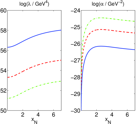
Figure 1: Illustrating the relationships between the brane tension, $\lambda$, the Gauss–Bonnet coupling parameter, $\alpha$, and the value of $x_{N}$ that arise after COBE normalization of the scalar perturbation amplitude. The solid lines correspond to $\beta^{2}=10$, the dashed lines to $\beta^{2}=100$ and the dot–dashed lines to $\beta^{2}=500$. The value of $x_{N}$ was evaluated 70 e–folds before the end of inflation and the constraints are not significantly altered by considering lower values of $N$ such as $N=50$.

4.2 Predictions for the observables

In determining the value of the spectral index, $n_{S}$, and its running, $dn_{S}/d\ln k$, we observe from Eq. (38) that the combination, $\alpha\lambda\beta^{4}$, depends explicitly only on the value of $x_{N}$ for a given value of $N$. Moreover, this combination of parameters appears directly in the expressions (30) and (31) for the slow–roll parameters. It follows, therefore, that substituting Eq. (38) into Eqs. (30) and (31) implies that the slow–roll parameters can be related directly to the value of $x_{N}$ independently of the slope of the potential $\beta$:

$$\epsilon = \frac{1}{3}~{}\frac{f(x_{N})}{N+1}~{}\frac{\sinh(2x_{N}/3)\,\sinh x_{N}\,\tanh x_{N}}{\left[\cosh(2x_{N}/3)-1\right]^{2}}\,,$$ (40)

$$\eta = \frac{f(x_{N})}{N+1}~{}\frac{\sinh x_{N}}{\cosh(2x_{N}/3)-1}\,.$$ (41)

Eqs. (40) and (41) may then be substituted into Eqs. (23) and (24), thereby relating the spectral index and its running directly to $x_{N}$. Fig. 2 illustrates the dependence of these two parameters on $x_{N}$. We observe that there is a lower limit of $n_{S}=1-4/(N+1)=0.944$, corresponding to the value predicted in the low energy (RSII) limit of steep inflation (i.e. when $\alpha\rightarrow 0$) [23]. The spectral index approaches unity if the $N$th e–fold before the end of inflation occurred in the high energy limit $x_{N}\gg 1$. Similarly, the expected value for the running of the spectral index $dn_{S}/d\ln k=-4/(N+1)^{2}=-7.9\times 10^{-4}$ is found in the limit $x_{N}\ll 1$ [29].

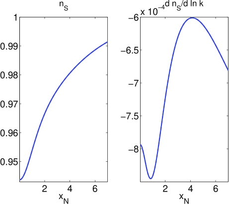
Figure 2: Illustrating the relationships between the spectral index, $n_{S}$, and its running, $d\ln n_{S}/d\ln k$, and the value of $x_{N}$ that arise after COBE normalization of the scalar perturbation amplitude. The value of $x_{N}$ was evaluated 70 e–folds before the end of inflation.

Our approach thus far in this Section has been to choose a value of $x_{N}$ for a given value of $N$, where the latter is chosen so that the horizon problem is automatically satisfied. However, there are two consistency checks that must be made to ensure that the above analysis is self–consistent. Firstly, one must ensure that inflation had indeed started by the time $x=x_{N}$. In other words, we must verify that the slow roll parameters are always less than unity in the range $x_{\rm end}<x<x_{N}$ for a chosen $x_{N}$. Fig. 3 verifies that the $\epsilon$ and $\eta$ parameters indeed satisfy this requirement.

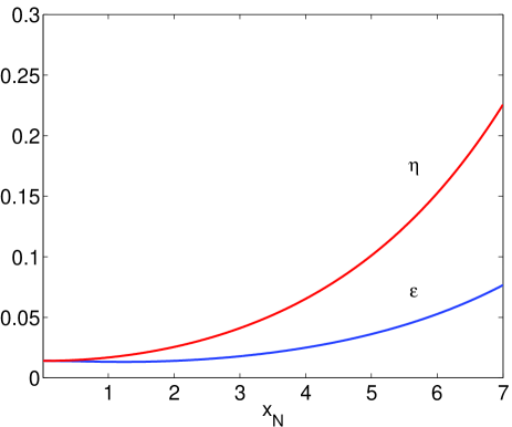
Figure 3: Illustrating the variation of the slow–roll parameters, $\epsilon$ and $\eta$, on $x_{N}$.

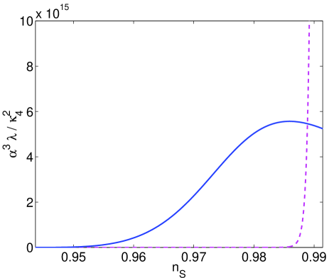
Figure 4: Illustrating the relationship (solid line) between $\alpha^{3}\lambda/\kappa_{4}^{2}$ and the spectral index, $n_{S}$, consistent with the COBE normalization constraint. The dashed line represents the critical case where the Planckian limit (42) is just satisfied. The region of parameter space consistent with this constraint is located above and to the left of this line. This results in an upper limit on the allowed value of the spectral index of $n_{S}\approx 0.989$.

Secondly, in the present scenario, the assumption that the scalar field is confined to the brane becomes unreliable if the energy density of the inflaton field exceeds the five–dimensional Planck scale. We must therefore impose the constraint $\rho<\kappa_{5}^{-8/3}$ and this leads to a lower limit on the allowed value of $\alpha^{3}\lambda$ for a given $x_{N}$:

$$\alpha^{3}\lambda>48\kappa_{4}^{2}\sinh^{6}x_{N}\,.$$ (42)

The constraint (42) effectively results in an upper limit on the allowed value of the spectral index, as follows from Fig. 4. This limit can be quantified by noting that $\alpha^{3}\lambda$ can be related directly to $x_{N}$ independently of the value of $\beta$ by combining Eq. (38) with Eq. (39). It follows that

$$\alpha^{3}\lambda=\frac{27\times 10^{16}}{256\pi^{4}}~{}\kappa_{4}^{2}~{}\left(\frac{N+1}{f(x_{N})}\right)^{2}~{}\frac{\left[\cosh(2x_{N}/3)-1\right]^{6}}{\sinh^{4}(x_{N})}\,,$$ (43)

and, since Fig. 2 implies that the correspondence between $x_{N}$ and $n_{S}$ is one–to–one, we may relate $\alpha^{3}\lambda/\kappa_{4}^{2}$ directly to $n_{S}$. The correspondence is shown in Fig. 4. Similarly, we may infer the region of parameter space consistent with the Planck limit (42) and this is illustrated by the dashed line in Fig. 4. We verify that the constraint $\rho<\kappa_{5}^{-8/3}$ breaks down for $n_{S}\geq 0.989$ or, equivalently, for $x_{N}\geq 6$. Thus, we predict that for this model, the allowed values of the spectral index and its running are bounded both from above and below. For example, in the specific case where $N=70$, we conclude that

$$0.944\leq n_{S}\leq 0.989\,,$$ (44)

$$-0.85\times 10^{-3}\leq\frac{dn_{S}}{d\ln k}\leq-0.60\times 10^{-3}\,.$$ (45)

These results are not significantly altered by reducing the total number of e–folds to $N=50$. The sensitivity of the constraints on the number of e–folds before the end of inflation is summarized in Table 1.

$N$	$n_{S}$	$-dn_{S}/d\ln k\times 10^{3}$
10	0.636 – 0.915	25.0 – 35.2
20	0.809 – 0.958	6.87 – 9.66
30	0.871 – 0.972	3.15 – 4.43
40	0.902 – 0.980	1.80 – 2.53
50	0.922 – 0.984	1.16 – 1.63
60	0.934 – 0.987	0.81 – 1.14
70	0.944 – 0.989	0.60 – 0.85

Table 1: The allowed values of the spectral index, $n_{S}$, and its running, $dn_{S}/d\ln k$, is weakly dependent on $N$, at least for $N\geq 40$.

5 Summary and discussion

In this paper, we have considered how the inclusion of a Gauss–Bonnet term in the bulk theory influences inflationary cosmology within the context of the Randall–Sundrum type II braneworld scenario. We have found that such a term can have a significant effect on the observational consequences of the scenario. In particular, we have focused on steep inflation, where the accelerated expansion of the braneworld is driven by an exponential potential with a logarithmic slope, $\beta\gg 1$. The effects of the Gauss–Bonnet contribution on the brane dynamics become significant at high energies and result in a density perturbation spectrum that can be very close to the scale–invariant (Harrison–Zeldovich) form. This is interesting given that steep exponential potentials arise in a number of M–theory inspired models [41]. Moreover, the numerical values of the spectral index and of its running are determined by the Gauss–Bonnet coupling parameter, $\alpha$, and the brane tension $\lambda$ (or, equivalently, the bulk cosmological constant, $\Lambda$) and are independent of the slope of the potential, $\beta$.

We found that the value for the running of the spectral index is of the order $dn_{S}/d\ln k\approx-10^{-3}$. Although preliminary analyses of the recent WMAP data have favoured somewhat smaller values [1], different authors have found little evidence for $dn_{S}/d\ln k\neq 0$ [40]. Nevertheless, improved observations will yield further information on the shape of the power spectrum and, consequently, on the validity of the model developed in the present work.

An important question that arises is how the spectrum of tensor (gravitational wave) perturbations is altered by the Gauss–Bonnet term. The calculation of the tensor perturbations in braneworld cosmology is more involved than that of the scalar perturbations, because the former extend into the bulk [42]. The equation of motion for the tensor modes is derived from the linear perturbations of the bulk field equations, but the linearly perturbed junction conditions impose a boundary condition on the modes at the location of the brane. A detailed study of these equations is beyond the scope of the present work. However, the model we have considered predicts a potentially detectable signal of long–wavelength gravitational waves in the absence of the Gauss–Bonnet term [23, 24, 25] and it would be interesting to investigate whether such a prediction is sensitive to the Gauss–Bonnet contribution. There is also the related question of whether the relationship between the scalar and tensor spectra is altered. In general, the two spectra are not independent and are related through a “consistency” relation, where the ratio of the amplitudes of the tensor and scalar perturbations is uniquely determined by the spectral index of the tensor spectrum. Such a relation represents a potentially observable signature of single-field inflationary models [38]. It was recently shown that in a number of braneworld models, the consistency equation takes precisely the same form as that of standard inflationary cosmology [24, 43]. This raises the question of whether the Gauss–Bonnet contribution is able to lift the degeneracy.

Finally, we conclude by highlighting a further consequence of the Gauss–Bonnet contribution on braneworld inflation. In Section 3.1, it was shown that at sufficiently high energies, the condition for inflation is that the pressure of matter on the brane should be negative, $p<0$. This conclusion may have implications for cosmological models dominated by a tachyon field. Following the work of Sen in understanding the role of the tachyon condensate in string theory [44], there has been considerable interest recently in developing models of inflation driven by such a field, and a recent discussion of the prospects and problems associated with tachyon cosmology was presented by Gibbons [45]. The dynamics of a time–dependent and homogeneous tachyon field, $T$, may be described by the effective lagrangian ${\cal{L}}=-U(T)[1-\dot{T}^{2}]^{1/2}$, where $U(T)$ represents the tachyon potential. This implies that the pressure of such a field is given by

$$p=-U(T)\sqrt{1-\dot{T}^{2}}\,,$$ (46)

and is negative–definite for a positive–definite potential, $U>0$. Thus, if we consider the tachyon as a degree of freedom on the brane, the above discussion indicates that a Gauss–Bonnet contribution may allow inflation to proceed at sufficiently high energies with only a very weak dependence on the functional form of the tachyon potential. It would be interesting to explore this possibility further.

References

- [1] D. N. Spergel et al., astro-ph/0302209; H. V. Peiris et al., astro-ph/0302225.
- [2] S. L. Bridle, A. M. Lewis, J. Weller, and G. Efstathiou, astro-ph/0302306.
- [3] A. A. Starobinsky, Phys. Lett. B 91, 99 (1980); A. H. Guth, Phys. Rev. D. 23, 347 (1981); A. Albrecht and P. J. Steinhardt, Phys. Rev. Lett. 48, 1220 (1982); S. W. Hawking and I. G. Moss, Phys. Lett. B 110, 35 (1982); A. D. Linde, Phys. Lett. B 108, 389 (1982); A. D. Linde, Phys. Lett. B 129, 177 (1983).
- [4] V. Mukhanov and G. Chibisov, Pis’ma Zh. Eksp. Teor. Fiz. 33, 549 (1981) [JETP Lett. 33, 532 (1981), astro-ph/0303077]; A. H. Guth and S. Y. Pi, Phys. Rev. Lett. 49, 1110 (1982); S. W. Hawking, Phys. Lett. B 115, 295 (1982); A. A. Starobinsky, Phys. Lett. B 117, 175 (1982); A. D. Linde, Phys. Lett. B 116, 335 (1982); J. M. Bardeen, P. J. Steinhardt, and M. S. Turner, Phys. Rev. D 28, 679 (1983).
- [5] A. R. Liddle and D. H. Lyth, Cosmological Inflation and Large-Scale Structure (Cambridge University Press, Cambridge, 2000).
- [6] J. Polchinski, String Theory (2 Vols., Cambridge University Press, Cambridge, 1998).
- [7] J. E. Lidsey, D. Wands, and E. J. Copeland, Phys. Rep. 337, 343 (2000); M. Gasperini and G. Veneziano, Phys. Rep. 373, 1 (2003); M. Quevedo, hep-th/0210292.
- [8] K. Akama, Lect. Notes Phys. 176, 267 (1982), hep-th/0001113; V. A. Rubakov and M. E. Shaposhnikov, Phys. Lett. B 125, 136 (1983); M. Visser, Phys. Lett. B 159, 22 (1985); P. Hořava and E. Witten, Nucl. Phys. B 460, 506 (1996); P. Hořava and E. Witten, Nucl. Phys. B 475, 94 (1996); N. Arkani–Hamed, S. Dimopoulos, and G. Dvali, Phys. Lett. B 429, 263 (1998); I. Antoniadis, N. Arkani–Hamed, S. Dimopoulos, and G. Dvali, Phys. Lett. B 436, 257 (1998); L. Randall and R. Sundrum, Phys. Rev. Lett. 83, 3370 (1999); A. Lukas, B. A. Ovrut, K. S. Stelle, and D. Waldram, Phys. Rev. D 59, 086001 (1999); A. Lukas, B. A. Ovrut, and D. Waldram, Phys. Rev. D 60, 086001 (1999); M. Gogberashvili, Europhys. Lett. 49, 396 (2000).
- [9] L. Randall and R. Sundrum, Phys. Rev. Lett. 83, 4690 (1999).
- [10] J. M. Maldacena, Adv. Theor. Math. Phys. 2, 231 (1998); E. Witten, Adv. Theor. Math. Phys. 2, 505 (1998); S. Gubser, I. Klebanov, and A. Polyakov, Phys. Lett. B 428, 105 (1998); O. Aharony, S. Gubser, J. Maldacena, H. Ooguri, and Y. Oz, Phys. Rep. 323, 183 (2000).
- [11] S. W. Hawking, T. Hertog, and H. Reall, Phys. Rev. D 62 043501 (2000); S. Nojiri, S. D. Odintsov, and S. Zerbini, Phys. Rev. D 62 064006 (2000); S. Nojiri and S. Odintsov, Phys. Lett. B 484, 119 (2000); L. Anchordoqui, C. Nunez, and K. Olsen, J. High Energy Phys. Phys. 10, 050 (2000); S. Nojiri and S. Odintsov, Phys. Lett. B 494, 135 (2000); S. Gubser, Phys. Rev. D 63, 084017 (2001); T. Shiromizu and D. Ida, Phys. Rev. D 64, 044015 (2001).
- [12] A. Fayyazuddin and M. Spalinski, Nucl. Phys. B 535, 219 (1998); O. Aharony, A. Fayyazuddin, and J. Maldacena, J. High Energy Phys. 07, 013 (1998).
- [13] S. Nojiri and S. D. Odintsov, J. High Energy Phys. 07, 049 (2000); M. Giovannini, Phys. Rev. D 63, 064011 (2001); S. Mukohyama, Phys. Rev. D 63, 104025 (2001); G. Kofinas, J. High Energy Phys. 08, 034 (2001); S. Nojiri, S. D. Odintsov, and S. Ogushi, Int. J. Mod. Phys. A 16, 5085 (2001); S. Nojiri, S. D. Odintsov, and S. Ogushi, Phys. Rev. D 65, 023521 (2002).
- [14] J. E. Kim, B. Kyae, and H. M. Lee, Phys. Rev. D 62, 045013 (2000); N. Deruelle and T. Dolezel, Phys. Rev. D 62, 103502 (2000); I. Low and A. Zee, Nucl. Phys. B 585, 395 (2000); O. Corradini and Z. Kakushadze, Phys. Lett. B 494, 302 (2000); J. E. Kim, B. Kyae, and H. M. Lee, Nucl. Phys. B 582, 296 (2000); Erratum–ibid B 591, 587 (2000); J. E. Kim and H. M. Lee, Nucl. Phys. B 602, 346 (2001); B. Abdesselam and N. Mohammedi, Phys. Rev. D 65, 084018 (2002); C. Germani and C. F. Sopuerta, Phys. Rev. Lett. 88, 231101 (2002); J. E. Lidsey, S. Nojiri, and S. D. Odintsov, J. High Energy Phys. 06, 026 (2002).
- [15] N. E. Mavromatos and J. Rizos, Phys. Rev. D 62, 124004 (2000); I. P. Neupane, J. High Energy Phys. 09, 040 (2000); I. P. Neupane, Phys. Lett. B 512, 137 (2001); K. A. Meissner and M. Olechowski, Phys. Rev. Lett. 86, 3708 (2001); Y. M. Cho, I. Neupane, and P. S. Wesson, Nucl. Phys. B 621, 388 (2002).
- [16] C. Charmousis and J. Dufaux, hep-th/0202107.
- [17] S. C. Davis, hep-th/0208205.
- [18] E. Gravanis and S. Willison, hep-th/0209076.
- [19] P. Binetruy, C. Charmousis, S. C. Davis, and J. Dufaux, Phys. Lett. B 544, 183 (2002).
- [20] B. Zwiebach, Phys. Lett. B 156, 315 (1985); A. Sen, Phys. Rev. Lett. 55, 1846 (1985); R. R. Metsaev and A. A. Tseytlin, Nucl. Phys. B 293, 385 (1987).
- [21] D. G. Boulware and S. Deser, Phys. Rev. Lett. 55, 2656 (1985).
- [22] N. Deruelle and J. Madore, Mod. Phys. Lett. A 1, 237 (1986); N. Deruelle and L. Farina–Busto, Phys. Rev. D 41, 3696 (1990).
- [23] E. J. Copeland, A. R. Liddle, and J. E. Lidsey, Phys. Rev. D 64, 023509 (2001).
- [24] G. Huey and J. E. Lidsey, Phys. Lett. B 514, 217 (2001).
- [25] V. Sahni, M. Sami, and T. Souradeep, Phys. Rev. D 65, 023518 (2002).
- [26] J. E. Lidsey, T. Matos, and L. A. Urena–Lopez, Phys. Rev. D 66, 023514 (2002).
- [27] A. R. Liddle and L. A. Urena–Lopez, astro-ph/0302054.
- [28] R. Maartens, D. Wands, B. Bassett, and I. Heard, Phys. Rev. D 62, 041301 (2000).
- [29] N. J. Nunes and E. J. Copeland, Phys. Rev. D 66, 043524 (2002).
- [30] N. Goheer and P. Dunsby, Phys. Rev. D 66, 043527 (2002).
- [31] E. I. Guendelman, Mod. Phys. Lett. A 14, 1043 (1999).
- [32] E. I. Guendelman and O. Katz, gr-qc/0211095.
- [33] R. C. Myers, Phys. Rev. D 36, 392 (1987).
- [34] P. Kraus, J. High Energy Phys. 12, 011 (1999); D. Ida, J. High Energy Phys. 09, 014 (2000).
- [35] R. G. Cai, Phys. Rev. D 65, 084014 (2002).
- [36] P. Binétruy, C. Deffayet, and D. Langlois, Nucl. Phys. B 565, 269 (2000); P. Binétruy, C. Deffayet, U. Ellwanger, and D. Langlois, Phys. Lett. B 477, 285 (2000); E. E. Flanagan, S. -H. Tye, and I. Wasserman, Phys. Rev. D 62, 044039 (2000); J. M. Cline, C. Grojean, and G. Servant, Phys. Rev. Lett. 83, 4245 (1999); C. Cśaki, M. Graesser, C. Kolda, and J. Terning, Phys. Lett. B 462, 34 (1999).
- [37] D. Wands, K. A. Malik, D. H. Lyth, and A. R. Liddle, Phys. Rev. D 62, 043527 (2000).
- [38] J. E. Lidsey, A. R. Liddle, E. W. Kolb, E. J. Copeland, T. Barreiro, and M. Abney, Rev. Mod. Phys. 69, 373 (1997).
- [39] E. F. Bunn, A. R. Liddle, and M. White, Phys. Rev. D 54, 5917R (1996); E. F. Bunn and M. White, Astrophys. J. 480, 6 (1997).
- [40] S. L. Bridle, A. M. Lewis, J. Weller and G. Efstathiou, astro-ph/0302306; U. Seljak, P. McDonald and A. Makarov, astro-ph/0302571.
- [41] G. T. Horowitz, I. Low, and A. Zee, Phys. Rev. D 62, 086005 (2000); T. Barreiro, B. de Carlos, and N. J. Nunes, Phys. Lett. B 497, 136 (2001).
- [42] D. Langlois, R. Maartens, and D. Wands, Phys. Lett. B 489, 259 (2000).
- [43] G. Huey and J. E. Lidsey, Phys. Rev. D 66, 043514 (2002); G. F. Giudice, E. W. Kolb, J. Lesgourgues, and A. Riotto, Phys. Rev. D 66, 083512 (2002).
- [44] A. Sen, J. High Energy Phys. 04, 048 (2002); A. Sen, J. High Energy Phys. 07, 065 (2002).
- [45] G. W. Gibbons, hep-th/0301117.