Abstract

Dust grains have been detected in various astronomical objects. Interpretation of observations of dusty objects includes three components: 1) determination of the materials which can exist in the solid phase and the measurements or acquisition of their optical constants; 2) selection of the light scattering theory in order to convert the optical constants into the optical properties of particles; and 3) the proper choice of the object model which includes, in particular, the correct treatment of the radiative transfer effects. The current state of the components of dust modeling and the reliability of information obtained on the cosmic dust from transmitted, scattered and emitted radiation are discussed.

1 Introduction

1.1 Observations

Dust grains have been detected in almost all astronomical objects from the local environment of the Earth to very distant galaxies and quasars. The interaction of radiation with grains includes two main processes: dust grains scatter and absorb radiation. The scattered radiation has the same wavelength as the incident one and can propagate in any direction. The radiation absorbed by a grain is transformed into its thermal energy and the particle emits at wavelengths usually longer than the absorbed radiation. Both processes contribute to extinction when the radiation from celestial bodies is attenuated by the foreground dust in the line of sight, i.e.

Extinction = scattering + absorption.

In general, it is possible to investigate the processes of extinction, scattering and emission of radiation by cosmic dust. Extinction is observed when the light is scattered at the scattering angle $\Theta=0^{\circ}$ (forward-transmitted radiation). Corresponding observational phenomena are interstellar extinction and polarization. In the case when the scattering dominates, an observer sees the radiation scattered at different angles from $\Theta=0^{\circ}$ to $\Theta=180^{\circ}$. The scattered radiation comes from the comets, zodiacal light, reflection nebulae, circumstellar shells, galaxies. Dust emission occurs in the H II regions, circumstellar shells, interstellar clouds, galaxies, etc.

1.2 Modeling

Interpretation of observations of dusty objects can be divided into three steps. By analogy with cooking, the “kitchen of dust modeling” would outline three primary factors to prepare this dish:

1. laying-in provision

   The primary task is to find elements which can be converted into the solid species in the circumstellar/interstellar conditions and to determine the resulting materials. The next task is to find or to measure optical constants (refractive indices) of the materials under consideration.

2. choice of equipment

   Selection of light scattering theory (“equipment”) is an essential aspect in dust modeling. The chosen method must provide the possibility of reproducing the most significant features of the observational phenomenon and to work rather fast in order to give results in a reasonable time.

3. cooking

   This most important part of the procedure is related to the skill of the cook (modeler) and includes not only a selection of provision and equipment but also a proper choice of the method of cooking — object modeling.

Lastly, one needs to taste the prepared dish, i.e. to compare the model with observations. The latter are performed with a limited accuracy which imposes a corresponding limitation on the claims of the model. From another point of view, a very complicated and detailed model with many parameters is ambiguous in principle. Further complicating the model, one should not forget about the principle of optical equivalence introduced by George Gabriel Stokes 150 years ago:

It is impossible to distinguish two beams which are the sum of non-coherent simple waves if they have the same Stokes parameters.

So, a judicious restriction on the detailed elaboration of different components in dust modeling should be found.

2 Abundances and optical constants

2.1 Element abundances and depletions

Ultraviolet (UV) and optical absorption-line studies have shown that the interstellar (gas-phase) abundances of many elements are lower than cosmic (reference) abundances. The rest of the elements is assumed to be locked in solid particles. The depletion of an element X is defined by

$$D_{\rm X}=\left.\left[\frac{\rm X}{\rm H}\right]_{\rm g}\right/\left[\frac{\rm X}{\rm H}\right]_{\rm cosmic},$$ (1)

where [X/H] is an abundance of element X relative to that of hydrogen. Here X (or $N_{\rm X}$) and H (or $N_{\rm H}=N_{{\rm HI}}+2N_{\rm H_{2}}$) are the column densities of an element X and hydrogen in a given direction. The abundances by number are usually expressed as the number of X atoms per $10^{6}$ hydrogen nuclei (particles per million, ppm, hereafter).

For a long time, the reference abundances were assumed to be equal to solar abundances. However, Snow and Witt [49] found that many species in cluster and field B stars, and in young F and G stars were significantly underabundant (by a factor of 1.5–2.0) relative to the Sun. The old (solar) and new (stellar) abundances for the five main elements forming cosmic dust grains are as follows: C (398ppm/214ppm), O (851ppm/457ppm), Mg (38ppm/25ppm), Si (35.5ppm/18.6ppm) and Fe (46.8ppm/27ppm). New abundances limited the number of atoms incorporated into dust particles. For example, the dust-phase abundances in the line of sight to the star $\zeta$ Oph are 79 ppm for C, 126 ppm for O, 23 ppm for Mg, 17 ppm for Si and 27 ppm for Fe. The most critical situation occurs for carbon which is the main component of many dust models. The inability to explain the observed interstellar extinction using the amount of carbon available in the solid phase resulted in so called “carbon crisis” which has not been resolved up to now.

2.2 Refractive indices and their mixing

The complex refractive indices ($m$) or dielectric functions ($\varepsilon$) of solids are called optical constants. The refractive index is written in the form $m=n(1+\varkappa i)$ or $m=n+ki$, where $k=n\varkappa\geq 0$. The sign of the imaginary part of the refractive index is opposite to that of the time-dependent multiplier in the presentation of fields. Note that in the book of van de Hulst [52] the refractive index is chosen as $m=n-ki$ whereas in the book of Bohren and Huffman [3] as $m=n+ki$.

The physical sense of $n$ and $k$ becomes clear if one considers the solution to the wave equations in an absorbing medium which is performed in the Cartesian coordinate system $xyz$. For an electric field propagating, for example, in the $z$-direction, we have

$$\vec{E}=\vec{E}_{0}\exp\left(-\frac{\omega}{c}kz\right)\exp\left[-i\omega\left(t-\frac{nz}{c}\right)\right],$$ (2)

where $\omega=2\pi\nu=2\pi c/\lambda$ is the circular frequency, $c$ the speed of light, $t$ time. As seen from Eq. (2), the imaginary part $k$ (often named the extinction coefficient or index) characterizes damping or absorption of the wave. The real part $n$ (the refraction index) determines the phase velocity of the wave in the medium, $v_{\rm phase}=c/n$.

The real and imaginary parts of the optical constants are not independent and may be calculated one from another using the Kramers–Kronig relations. When applied to $n$ and $k$, the relations are

$$n(\omega)=1+\frac{2}{\pi}{\mathcal{P}}\int_{0}^{\infty}\frac{\Omega k(\Omega)}{\Omega^{2}-\omega^{2}}\,{\rm d}\Omega,$$ (3)

$$k(\omega)=-\frac{2\omega}{\pi}{\mathcal{P}}\int_{0}^{\infty}\frac{n(\Omega)}{\Omega^{2}-\omega^{2}}\,{\rm d}\Omega,$$ (4)

where $\cal{P}$ denotes the principal part of the integral. Equations (3) and (4) allow one to make some conclusions on the behavior of the optical constants in different wavelength ranges. In particular, it is impossible to have a material with $k=0$ at all wavelengths because in this case the radiation does not interact with the material ($n=1$ everywhere).

The optical constants for amorphous carbon plotted in Fig. 1 allow us to understand the relation between the real and imaginary parts of the refractive indices. In particular, the limiting and asymptotic values of $n$ and $k$ are clearly seen. Note that the absorption features appear as loops in the $k-n$ diagrams. In the last few years, special measurements of the optical constants for cosmic dust analogues have been made. These data are being collected in the database of optical constants for astronomy (Jena–Petersburg Database of Optical Constants, JPDOC; see [20], [25] for details).

Figure 1.  : Refractive indices of amorphous carbon calculated with the Bruggeman mixing rule for a different fraction of vacuum ($f$=0–0.5). The values of wavelengths in ${\mu}\rm{m}$ are indicated.

The conditions in which cosmic dust grains originate, grow and evolve should lead to the formation of heterogeneous particles with complicated structure. The problem of electromagnetic scattering by such composite particles is so difficult that a practical, real-time solution is currently unfathomable, in particular keeping in mind the unknown real structure of grains. Therefore, the thought of obtaining the optical properties of heterogeneous particles using homogeneous particles with effective dielectric functions $\varepsilon_{\rm eff}$ found from a mixing rule (generally called an Effective Medium Theory; EMT) is an extremely attractive proposition.

Many different mixing rules exist (see [8] and [47] for a review). They are rediscovered from time to time and sometimes can be obtained one from another. The most popular EMTs are the classical mixing rules of (Maxwell) Garnett and Bruggeman. In the case of spherical inclusions and a two-component medium the effective dielectric constant may be calculated easily from the dielectric permittivities $\varepsilon_{1}$, $\varepsilon_{2}$ and volume fractions $f$, $1-f$ of the components. The Garnett rule assumes that one material is a matrix (host material) in which the other material is embedded. It is written in the following form:

$$\varepsilon_{\rm eff}=\varepsilon_{2}\left[1+\frac{3f\frac{\varepsilon_{1}-\varepsilon_{\rm 2}}{\varepsilon_{1}+2\varepsilon_{\rm 2}}}{1-f\frac{\varepsilon_{1}-\varepsilon_{\rm 2}}{\varepsilon_{1}+2\varepsilon_{\rm 2}}}\right].$$ (5)

When the roles of the inclusion and the host material are reversed, the inverse Garnett rule is obtained

$$\varepsilon_{\rm eff}=\varepsilon_{1}\left[1+\frac{3(1-f)\frac{\varepsilon_{2}-\varepsilon_{\rm 1}}{\varepsilon_{2}+2\varepsilon_{\rm 1}}}{1-(1-f)\frac{\varepsilon_{2}-\varepsilon_{\rm 1}}{\varepsilon_{2}+2\varepsilon_{\rm 1}}}\right].$$ (6)

The Bruggeman rule is symmetric with respect to the interchange of materials

$$f\frac{\varepsilon_{1}-\varepsilon_{\rm eff}}{\varepsilon_{1}+2\varepsilon_{\rm eff}}+(1-f)\frac{\varepsilon_{2}-\varepsilon_{\rm eff}}{\varepsilon_{2}+2\varepsilon_{\rm eff}}=0.$$ (7)

Figure 1 shows variations of the refractive indices of amorphous carbon calculated with the Bruggeman mixing rule for a different fraction of vacuum.

A special question is the range of applicability of the EMTs. A general conclusion made from calculations (see [53], [67]) is that an EMT agrees well with the exact theory if the inclusions are Rayleigh and their volume fraction $f$ is below $\sim$ 40–60%. In the case of non-Rayleigh inclusions, apparently, $f$ should not exceed $\sim$10%. Kolokolova and Gustafson [30] performed a comprehensive study of the possibility of applying nine mixing rules comparing calculations for organic spheres with silicate inclusions using microwave analog experiments. They recommend the use of EMTs if the volume fraction of inclusions is not more than 10%.

3 Light scattering theories

When the optical constants are chosen, they can be converted into optical properties of particles: various cross-sections, scattering matrix, etc. using a light scattering theory. Theories of light scattering by particles may make it possible to calculate the following:
1) intensity and polarization of radiation scattered in any direction;
2) energy absorbed or emitted by a grain and to find its temperature;
3) emission spectra of dusty objects;
4) radiation pressure force on dust grains which frequently determines their motion.

Theoretical approaches to solve the light scattering problem are divided into exact methods and approximations by their dependence on the following:
1) the size parameter $x=2\pi r/\lambda$, where $r$ is the typical size of a particle (e.g., the radius of the equi-volume sphere) and $\lambda$ the wavelength of incident radiation in the surrounding medium;
2) the module of the difference between the refractive index and unity $|m-1|$;
3) the phase shift $\rho=2x|m-1|$.
Approximations may be applicable if at least two of these quantities are much smaller or much larger than unity [52]. In particular, approximate approaches allow one to estimate the wavelength dependence of extinction cross-sections easily. The latter determine, for example, interstellar extinction $A(\lambda)$ (see Sect. 5.1). Multi-color observations show that $A(\lambda)\propto\lambda^{-1}$ in the visible part of the spectrum and no approximation predicts such a wavelength dependence. Therefore, astronomers in general are doomed to work with exact methods. Spherical grains do not explain the interstellar polarization and another feature required of the theory is the ability to treat non-spherical particles with sizes close to or larger than the radiation wavelength.

At present, only a few methods satisfy astronomical demands and three of them are widely used in astrophysical modeling. These are the separation of variables method for spheroids, the T-matrix method for axially symmetric particles, and some modifications of the method of momentum (and first of all the discrete dipole approximation, DDA).

The current state of methods and techniques of calculating light scattering by non-spherical particles are described in special issues of Journal of Quantitative Spectroscopy and Radiative Transfer [23], [32], [37], [54], review papers [27], [68] and the collective monograph [36]. A detailed description of different approximations can be found in [27], [29] and [40].

4 Objects’ models

In the modeling of dusty objects one needs to select not only optical constants and a light scattering approach, but also an appropriate model of the object. The model of a dusty object includes an appropriate choice of the spatial distribution of scatterers (dust grains) and illuminating sources and correct treatment of radiative-transfer effects.

Radiative transfer methods are rather conservative and making changes or modifications usually require tremendous efforts. As a result, the radiative transfer code available determines the final result of modeling, but different radiative transfer codes may give different results. During its long history, radiative transfer theory passed through several stages: analytical, semi-analytical and numerical. The problems which can be solved analytically are very simple ones like the fluxes from a sphere found in the Eddington approximation assuming grey opacity and the spherical phase function. Modern observational techniques give the spectral energy distributions, images and polarization maps of very complicated objects like fragmented molecular cloud cores, circumbinary and circumstellar disks. These data cannot be modeled without very complicated radiative transfer programs, and consideration of polarization usually requires application of Monte Carlo methodologies.

Some characteristics of radiative transfer programs created during the last 25 years and their applications to the interpretation of observed data on dusty cosmic objects are collected in Table 7 in [58]. The major part of the work mentions that these are based on two methods:
1) iterative schemes to solve the moment equations of the radiative transfer equation and
2) Monte Carlo simulation.
Standard applications include the following: circumstellar shells and envelopes around early (pre-main-sequence) and late-type stars and young stellar objects, reflection nebulae, interstellar clouds and globules, diffuse galactic light and in recent years galaxies and active galactic nuclei.

5 Interstellar extinction and polarization

5.1 Observations

Observational analysis of interstellar extinction and polarization is twofold: “in depth” and “in breadth”. The first involves examination of the wavelength dependence and gives information about the properties of interstellar grains. The second includes the study of the distribution of dust matter and relates to work on galactic structure.

The wavelength dependence of extinction $A(\lambda)$ is rather well established in the range from near-infrared (IR) to far-UV. It has often been represented using simple analytical formulae. The most recent analytical fitting of the extinction curves was obtained in [13]. Observations in the far-UV show that the growth of the interstellar extinction continues almost up to the Lyman limit [42]. At wavelengths shorter than 912 Å, the extinction is dominated by photo-ionization of atoms, not by the scattering and absorption by dust. In the extreme UV ($\lambda$ 100–912 Å), almost all radiation from distant objects is “consumed” by neutral hydrogen and helium in the close vicinity of the Sun. In the X-range, photo-ionization of other abundant atoms (C, N, O, etc.) becomes important. The resulting wavelength dependence of extinction in the diffuse interstellar medium is plotted in Fig. 2. It shows extinction cross-sections $\sigma_{\rm d}(\lambda)$ related to the column density of H-atoms, which can be found from the following expression (see [58] for details):

Figure 2.  : Extinction in the diffuse interstellar medium. The sources of the data are given in Table 9 in [58].

$$\sigma_{\rm d}(\lambda)=4.18\times 10^{-22}\,\frac{A(\lambda)}{A_{\rm V}}.$$ (8)

The coefficient in Eq. (8) was calculated for the ratio of the total extinction to the selective one $R_{\rm V}=A_{\rm V}/E{\rm(B-V)}=3.1$ and the gas to dust ratio ${N({\rm H})}/{E{\rm(B-V)}}=6.83\times 10^{21}\,{\rm atoms\,cm^{-2}\,mag^{-1}}$.

The phenomenon of interstellar linear polarization is connected to the effect of the linear dichroism of the interstellar medium which arises because of the presence of aligned non-spherical grains. Such particles produce different extinctions of light depending on the orientation of the electric vector of incident radiation relative to the particle axis. The wavelength dependence of polarization $P(\lambda)$ now is known in the spectral range $\lambda$ 0.12–12 ${\mu}\rm{m}$. The polarization degree usually has a maximum in visible and declines in the IR and UV (Fig. 3).

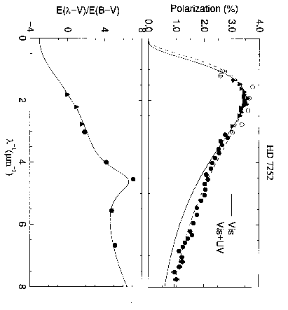
Figure 3.  : Polarization and extinction curves in the direction of the star HD 7252 (after [63]).

As a rule, the dependence $P(\lambda)$ is described by an empirical formula suggested by Serkowski [44]

$$P(\lambda)/P_{\rm max}=\exp[-K\ln^{2}(\lambda_{\rm max}/\lambda)].$$ (9)

Initially, the Serkowski’s curve had only two parameters: the maximum degree of polarization $P_{\rm max}$ and the wavelength corresponding to it $\lambda_{\rm max}$. The coefficient $K$ was chosen by Serkowski [44] to be equal to 1.15.

An example of the behavior of polarization is shown in Fig. 3. The solid curves fit the ground-based data using only Serkowski’s curve (Eq. (9)) and the relation $K=1.86\cdot\lambda_{\rm max}-0.10$ found in [65]. The interstellar polarization in the direction of HD 7252 ($\lambda_{\rm max}=0.52\,{\mu}\rm{m}$) displays a clear excess over the extrapolated curve (“super-Serkowski behavior”). Note that polarization features have been discovered in only a few directions in the Galaxy, although the bump near $\lambda 2175$ Å  is a common attribute of all extinction curves. In order to represent the wavelength dependence of polarization from IR to UV, Martin et al. [33] suggested a five-parameter interpolation formula consisting of two terms describing UV and visual-IR polarization. The result of fitting is shown by the dashed curve in Fig. 3.

Note also that historically the direction of starlight polarization is associated with the orientation of the plane-of-the-sky component of the interstellar magnetic field, $B_{\bot}$. The data of polarimetric surveys together with other observations like Zeeman splitting of the H I (21 cm) line are used to study the magnetic field structure at different scales.

5.2 Interpretation

The intensity of radiation after passing through a dust cloud $I(\lambda)$ is equal to

$$I(\lambda)=I_{\star}(\lambda)e^{-\tau_{\rm ext}(\lambda)},$$ (10)

where $I_{\star}(\lambda)$ is the source (star) intensity and $\tau(\lambda)$ the optical thickness along the line of sight. The interstellar extinction is

$$A(\lambda)=-2.5\log\frac{I(\lambda)}{I_{\star}(\lambda)}\approx 1.086\tau_{\rm ext}(\lambda).$$ (11)

For spherical particles of radius $r_{\rm s}$, we have

$$A(\lambda)=1.086\,\pi r_{\rm s}^{2}\,Q_{\rm ext}(m,r_{\rm s},\lambda)\,N_{\rm d}=1.086\,\pi r_{\rm s}^{2}\,Q_{\rm ext}(m,r_{\rm s},\lambda)\,n_{\rm d}\,D,$$ (12)

where $N_{\rm d}$ and $n_{\rm d}$ are the column and number densities of dust grains, correspondingly, and $D$ is the distance to the star. From Eq. (12) it follows that the wavelength dependence of interstellar extinction is determined completely by the wavelength dependence of the extinction efficiencies $Q_{\rm ext}$. Such a dependence is plotted in Fig. 4 for particles of astronomical silicate.

Figure 4.  : Wavelength dependence of the extinction efficiency factors for homogeneous spherical particles of different sizes consisting of astronomical silicate. The dashed segment shows the approximate wavelength dependence of the mean galactic extinction curve at optical wavelengths (after [58]).

Dust grains are considered to have some size distribution. Very often a grain size distribution like that suggested in [34] (“MRN”) $n(r_{\rm s})\propto r_{\rm s}^{-3.5}$ is used. In this case, the extinction is proportional to

$$A(\lambda)\propto\int Q_{\rm ext}(\lambda)\,r_{\rm s}^{-1.5}{\rm d}r_{\rm s}.$$ (13)

Figure 5 allows us to estimate the contribution of particles of different sizes to the extinction for a given wavelength (see Eq. (13)) if the distribution is like MRN.

Figure 5.  : Wavelength dependence of the integrand in Eq. (13) for homogeneous spherical particles of different sizes consisting of astronomical silicate.

From Fig. 4 the influence of the size and chemical composition of particles on the extinction for a given wavelength can be examined. In all cases, the rate of growth increases until we approach the first maximum of $Q_{\rm ext}(m,x)$. As follows from Fig. 4, spheres of astrosil with $r_{\rm s}\approx 0.1\,{\mu}\rm{m}$ can produce the dependence $A(\lambda)$ resembling the observed one. The same is possible for spheres of amorphous carbon of smaller radius (see discussion in [58]). So, from the wavelength dependence of extinction one can determine only the product of the typical particle size on refractive index but not the size or chemical composition of dust grains separately. It is also possible to show that particles of different structure (for example, with mantle or voids) as well as of different shape may represent the dependence of $A(\lambda)$ rather well. Thus, neither chemical composition, nor structure and shape of dust particles can be uniquely deduced from the wavelength dependence of the interstellar extinction.

Along with the wavelength dependence, it is important to reproduce the absolute value of extinction using the dust-phase abundances found for a given direction $[{\rm X}/{\rm H}]_{\rm d}$. These abundances can be expressed via
1) observed quantities: interstellar extinction $A_{\rm V}$ and hydrogen column density $N({\rm H})$;
2) model parameters: mass of constituents in a grain, the relative part of the element $X$ in the constituent $i$, density of grain material and relative volume of the constituent in a particle $V_{i}/V$; and
3) a calculated quantity: the ratio of the extinction cross-section to the particle volume $C_{\rm ext}/V$.
The last ratio must be maximal in order to produce the largest observed extinction and simultaneously to save the material. However, at the moment it is rather difficult to explain the carbon crisis using particles of different structure and shape (see discussion in [58]). For example, in order to explain the absolute extinction of the star $\zeta$ Oph (HD 149757; $A_{\rm V}=0\hbox{$.\!\!^{\rm m}$}94$) using homogeneous spherical particles, the minimum abundance of carbon must be 320 ppm in the case of amorphous carbon and 267 ppm in the case of graphite (the dust-phase value is 79 ppm, see Sect. 2.1). If the particles are of astrosil (MgFeSiO₄), 52.5 ppm of Fe, Mg and Si and 211 ppm of O are required. All these abundances are larger than those estimated from observations of dust-phase abundances. Possibly, the way to resolve the problem is a thorough analysis of cosmic abundances which probably are not the same in different galactic regions.

To model the interstellar polarization one needs to calculate the forward-transmitted radiation for an ensemble of non-spherical aligned dust grains. This procedure consists of two steps: 1) computing the extinction cross-sections for two polarization modes, and 2) averaging the cross-sections for given particle size and orientation distributions.

Let non-polarized stellar radiation passes through a dusty cloud with a homogeneous magnetic field. The angle between the line of sight and the magnetic field is $\Omega$ ($0\hbox{${}^{\circ}$}\leq\Omega\leq 90\hbox{${}^{\circ}$}$). As follows from observations and theoretical considerations [10], the magnetic field determines the direction of alignment of dust grains. The linear polarization produced by a rotating spheroidal particle is

$$\begin{array}[]{l}\displaystyle P(\lambda)=\int_{\varphi,\,\omega,\,\beta}\frac{1}{2}\left[C^{\rm TM}_{\rm ext}(m,r_{V},\lambda,a/b,\alpha)-C^{\rm TE}_{\rm ext}(...)\right]\times\\ \times\hat{f}[\xi(r_{V},\chi^{\prime\prime},n_{\rm H},B,T_{d},T_{g}),\beta]\,\cos 2\psi\,{\rm d}[\varphi,\omega,\beta]\cdot N_{d}\cdot 100\%,\end{array}$$

where $C^{\rm TM,\,TE}_{\rm ext}$ are the extinction cross-sections for two polarization modes, $N_{\rm d}$ the column density of dust grains. $\hat{f}(\xi,\beta)$ is the function of orientation, depending on the alignment parameter $\xi$ and the precession angle $\beta$.

Of special interest are the variations of the polarization in cold dark clouds and star-forming regions. It was found that in several dark clouds (L 1755, L 1506, B 216–217 [2]) the increase of polarization with growing extinction stops beginning at some value of $A_{\rm V}$. This fact may be related with the following:
1) optics of dust ($C^{\rm TM}_{\rm ext}\simeq C^{\rm TE}_{\rm ext}$ in Eq. (5.2));
2) physics of dust (no grain alignment);
3) object’s properties (line of sight is parallel to the direction of alignment, $\Omega\simeq 0^{\circ}$ or two or more clouds are present on the line of sight which leads to the cancellation of polarization).

Figure 6.      Polarization efficiency as a function of $x_{V}$ for prolate and oblate spheroids with $m=1.3+0.0i$ and $1.7+0.7i$, picket fence

orientation, $\alpha=90\hbox{${}^{\circ}$}$. The size/shape effects are illustrated (after [62]).

The proximity of cross-sections $C^{\rm TM}_{\rm ext}$ and $C^{\rm TE}_{\rm ext}$ may indicate that the shape of grains is more spherical in darker parts of clouds. In a like manner, the reduction of polarization occurs if the size of non-spherical particles becomes larger than the radiation wavelength (see Fig. 6). This Figure illustrates the behavior of the polarization efficiency $P/\tau$ (the upper/lower sign corresponds to prolate/oblate spheroids):

$$\frac{P(\lambda)}{\tau(\lambda)}=\pm\frac{C_{\rm pol}}{C_{\rm ext}}=\pm\frac{C^{\rm TM}_{\rm ext}-C^{\rm TE}_{\rm ext}}{C^{\rm TM}_{\rm ext}+C^{\rm TE}_{\rm ext}}\cdot 100\%=\pm\frac{Q^{\rm TM}_{\rm ext}-Q^{\rm TE}_{\rm ext}}{Q^{\rm TM}_{\rm ext}+Q^{\rm TE}_{\rm ext}}\cdot 100\%$$ (14)

for non-absorbing and absorbing spheroids for the case when a maximum polarization is expected (non-rotating particles, radiation propagates perpendicular to the symmetry/rotation axis of the spheroid, $\alpha=90\hbox{${}^{\circ}$}$). It is seen that relatively large particles produce no polarization independently of their shape. For absorbing particles, non-zero polarizations occur at smaller $x_{V}$ values than for non-absorbing ones. However, the position at which the ratio $P/\tau$ reaches a maximum is rather stable in every panel of Fig. 6 and is independent of $a/b$.

Figure 7.      Extinction and linear polarization factors, polarization efficiency and circular polarization factors as a function of $x_{V}$ for

prolate spheroids with $m=1.3+0.0i$ and $a/b=2$, picket fence orientation. The effect of variations of particle orientation is illustrated

(after [58]).

These results no longer remain valid when the radiation is incident obliquely as is demonstrated in Fig. 7. The angular dependence of the extinction and linear polarization factors in Eq. (14) differs: if $\alpha$ decreases, the position of the maximum for $Q_{\rm ext}$ shifts to smaller values of $x_{V}$ while that for $Q_{\rm pol}$ shifts to larger $x_{V}$ (Fig. 7, upper panels). As a result, the maximum polarization efficiency for prolate spheroids is reached at smaller $x_{V}$ in the case of tilted orientation (Fig. 7, lower left panel), and the picture is reversed for oblate particles (see [58]).

Thus, for particles larger than the radiation wavelength, the linear polarization is expected to be rather small. This does not allow one to distinguish between the particle properties like refractive index, shape, orientation. Even in the case of the most preferable orientation, large particles (possibly available in dark clouds) do not polarize the transmitted radiation significantly.

6 Scattered radiation

6.1 Observations

If a dusty object radiates at a given wavelength, scattered light is always present in its radiation. The amount may be negligible, but it exists. This is due to the fact that the particle albedo can never be equal to zero.

The necessary condition for the appearance of scattered radiation is the existence of a source of illumination. The spectrum of the scattered light generally resembles that of the source. However, the color of the reflection nebulae may be bluer or redder than that of the illuminating stars depending on the properties (primarily the size) of the dust grains and the scattering geometry (see [55] for discussion). The latter (i.e., the mutual position of an illuminating source, scattering volume and an observer) also strongly influences the observed polarization, which is the usual attribute of the scattered radiation. The degree of linear polarization in reflection nebulae may reach 50% and more. The typical intrinsic polarization in circumstellar shells is several percent, but may sometimes reach 20–30%. The centro-symmetric polarization pattern in nebulae is used to search for the positions of illuminating stars.

However, simple cases, like single scattering from one source, are not typical in astronomy. More often, complex or mixed cases are observed: attenuation of a part of the scattered volume by a foreground dust cloud, multiple scattering effects, etc. This leads to the appearance of so-called polarization null points on the polarization maps where a reversal of the polarization occurs, change of the sign of the polarization with wavelength, non-centrosymmetric structure of the polarization maps, variations of the positional angle of polarization with wavelength, or very high degrees of circular polarization (see [66] for references and discussion). Some of these features are seen in Fig. 8 where the polarimetric map of the circumstellar shell around the carbon star IRC +10 216 is shown.

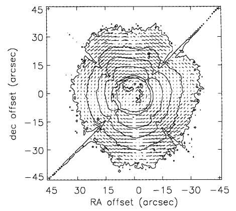
Figure 8.  : 2.2 ${\mu}\rm{m}$ polarimetric map constructed from a set of occulted, polarimetric images of IRC +10 216. The map is superimposed on a contour plot of an unpolarized image constructed from the same set of images (after [28]).

6.2 Interpretation

The process of light scattering is described in terms of the particle albedo and scattering matrix. But it is enough to calculate the first element of the scattering matrix $F_{11}$ (phase function) only if the polarization is not considered. Frequently, the phase function is used in the simplified form suggested by Henyey and Greenstein [21] and is parameterized by the asymmetry parameter $g$ (or $\langle\cos\Theta\rangle$). It varies from –1 (mirror particles) to 1 (all radiation is forward scattered). Note that mirror particles (with $g<0$) are very atypical because no grain material (with the exception of very small iron particles) gives at visual wavelengths a negative asymmetry parameter. Even pure conductors ($m=\infty$) have $g\approx-0.2$ [52].

In optically thin case the amount of observed scattered radiation is proportional to

$$I(\lambda)\propto I_{\star}(\lambda){[1-g(\lambda)]\Lambda(\lambda)}\tau_{\rm ext}(\lambda),$$ (15)

where $I_{\star}(\lambda)$ describes the power of the source, the quantities ${\Lambda}$ and $1-g(\lambda)$ characterize the ability of a particle to scatter the radiation and the scattering geometry, respectively, and the last multiplier $\tau_{\rm ext}(\lambda)$ is proportional to the extinction cross-section and the number of scatterers. It is evident that the incoming scattered radiation vanishes if $I_{\star}(\lambda),\Lambda(\lambda)$ or $\tau_{\rm ext}(\lambda)$ approaches zero or $g(\lambda)$ tends to unity.

Figure 9.      Wavelength dependence of the albedo, asymmetry parameter and the product of grain scattering characteristics given by

Eq. (15) for homogeneous spherical particles of different sizes consisting of astronomical silicate. The lower right panel allows one to

estimate the contribution of particles into scattered radiation if the size distribution is like MRN.

The standard behavior of particle albedo and asymmetry parameter is the following: $\Lambda\ll 1$ and $g\simeq 0$ for small size parameters (small sizes or large wavelengths), both characteristics grow with increasing particle size or decreasing the radiation wavelength and reach the asymptotic values for very large size parameters. The wavelength dependencies of $\Lambda$ and $g$ are shown in Fig. 9 (upper panels) for particles of astrosil. It is seen that the albedo of particles with $r_{\rm s}\geq 0.05\,{\mu}\rm{m}$ is rather high (up to $\sim$0.9) in a wide wavelength range and reduces in the far-UV. At the same time, the asymmetry parameter shows a tendency toward growth. So, we expect reduction of the role of scattered light in the UV in comparison with the visual part of spectrum. This is clearly seen at the lower left panel of Fig. 9 where the product $[1-g(\lambda)]\Lambda(\lambda)Q_{\rm ext}(\lambda)$ as given by Eq. (15) is plotted. The contribution of a particle of given size to the scattering occurs at some wavelength which correlates with the particle size (i.e. larger particles scatter radiation at longer wavelengths). But grains with radii $r_{\rm s}\mathrel{\mathchoice{\vbox{\offinterlineskip\halign{\hfil$\displaystyle#$\hfil\cr<\cr\sim\cr}}}{\vbox{\offinterlineskip\halign{\hfil$\textstyle#$\hfil\cr<\cr\sim\cr}}}{\vbox{\offinterlineskip\halign{\hfil$\scriptstyle#$\hfil\cr<\cr\sim\cr}}}{\vbox{\offinterlineskip\halign{\hfil$\scriptscriptstyle#$\hfil\cr<\cr\sim\cr}}}}0.01\,{\mu}\rm{m}$ hardly affect the scattered radiation. This conclusion remains valid if one considers size distributions like MRN (see the lower right panel of Fig. 9).

It is important to keep in mind that the albedo and asymmetry parameter cannot be determined from observations separately, but only in the form of a combination. Therefore, models with one fixed parameter and the other varying make little physical sense. The dependence of $\Lambda$ on $g$ is plotted in Fig. 10 for particles from astrosil and AC1. It is seen that some pairs of parameters correspond to no particles. The theoretical constraints on the albedo and asymmetry parameter were discussed by Chlewicki and Greenberg [7] who showed that some modeling results could not be represented in the optics of small particles.

Figure 10.      Albedo dependence on asymmetry parameter for homogeneous spherical particles of different sizes consisting of

astronomical silicate and amorphous carbon. The values of wavelength are given in ${\mu}\rm{m}$ for particle with $r_{\rm s}=0.02\,{\mu}\rm{m}$.

In general, the radiation scattered by aligned non-spherical particles has an azimuthal asymmetry that provokes a non-coincidence of the directions of the radiation pressure force and of the wave-vector of incident radiation [59]. Another consequence of the azimuthal asymmetry is the anisotropy of the phase function in the left/right direction. The geometry of the phase function in forward/backward and left/right directions may be characterized by two asymmetry parameters $g_{||}$ and $g_{\bot}$, respectively (see [57] for details). The values of radial asymmetry factor $g_{||}$ decrease with a growth of $\alpha$ when the path of radiation reduces from $2a\ (\alpha=0^{\circ})$ to $2b\ (\alpha=90^{\circ})$. The transversal asymmetry factor $g_{\bot}$ can be rather large and even exceeds the radial one. Because the geometry of light scattering by very elongated spheroids approaches that of infinite cylinders, such particles scatter more radiation “to the side” than in the forward direction.

At the same time, the albedo for large non-spherical particles becomes close to that of spheres. Our calculations made for particles with different absorption [62] demonstrate that the distinction of the albedo for spheres and spheroidal particles remains rather small (within $\sim 20\,\%$) if the ratio of the imaginary part of the refractive index to its real part $k/n\mathrel{\mathchoice{\vbox{\offinterlineskip\halign{\hfil$\displaystyle#$\hfil\cr>\cr\sim\cr}}}{\vbox{\offinterlineskip\halign{\hfil$\textstyle#$\hfil\cr>\cr\sim\cr}}}{\vbox{\offinterlineskip\halign{\hfil$\scriptstyle#$\hfil\cr>\cr\sim\cr}}}{\vbox{\offinterlineskip\halign{\hfil$\scriptscriptstyle#$\hfil\cr>\cr\sim\cr}}}}0.2-0.3$.

The difference in the single light scattering by a spherical particle and an aligned non-spherical particle are readily apparent in the behavior of the elements of the first column of the scattering matrix. These elements determine the scattered radiation if the incident radiation is non-polarized. In contrast to spheres, the scattering by non-spherical particles causes the rotation of the positional angle of linear polarization and produces circular polarization after the first scattering event. This is the result of non-zero elements $F_{31}$ and $F_{41}$ of the scattering matrix for aligned non-spherical particles. Thus, some observational features mentioned in Sect. 6.1 may be attributed to light scattering by non-spherical grains.

Figure 11.      The element $F_{11}$ and the ratios of elements of the scattering matrix $-F_{21}/F_{11}$, $F_{33}/F_{11}$ and $F_{43}/F_{11}$ for sphere, prolate

and oblate spheroids, $m=1.5+0.01i$, $x_{V}=5$, $\alpha=50^{\circ}$, $\Phi=0^{\circ}$. The influence of variations of particle shape is illustrated. Adapted

from [24].

The elements of the scattering matrix for spherical and spheroidal particles of the same size and refractive index are compared in Fig. 11. It shows that the major differences between spheres and spheroids as well as between prolate and oblate particles appear at large scattering angles. Such behavior is rather common (see [35] for discussion). Therefore, in order to investigate the shape effects, we need to observe an object located behind the illuminating source that occurs on occasion. However, a thin layer of the foreground dust can produce much more scattered radiation than background dust (see upper left panel in Fig. 11). So, it is rather difficult to diagnose the particle shape from scattered radiation in complex celestial objects.

7 Infrared radiation

7.1 Observations

As noted by Glass [17]: “The central astronomical role of dust is at its most evident in the infrared.” The observed IR and submillimeter emission from interstellar clouds, circumstellar envelopes, and galaxies is generally thermal emission of dust heated by stellar radiation or shock waves. The spectrum of dust emission is blackbody. Its shape is mainly determined by the properties of heating sources and the dust distribution around them. The individual characteristics of particles manifest themselves in different temperatures of metallic and dielectric grains and in a full manner as spectral features superimposed on continuum emission. The dust features are observed in absorption and emission and are the vibrational transitions in solid materials — constituents of grain cores and mantles (usually bending or stretching modes). The IR spectral features present the most reliable method of diagnostics of dust chemical composition. As a rule, the dust bands are rather weak and in order to find them the process of subtracting the continuum is required (see Fig. 12).

Figure 12.  : The ISO spectrum of the post-red supergiant star AFGL 4106 with the spline fit of continuum. The result of the subtraction of the spline fit continuum (dashed line in A) is shown in graph B. The result of the removal of the broad silicate features (dashed line in B) is given in graph C (after [39]).

The observed IR features attributed to the interstellar and circumstellar dust are collected in Table LABEL:dust_f. This is the updated version of Table 7 published in 1986 (see [56]) which included 24 features and was significantly enlarged after the discoveries made from the Infrared Space Observatory (ISO). First of all ISO contributed into the mid-IR where numerous emission features of crystalline silicates were found. They were identified with magnesium–iron silicates: pyroxenes (Mg_xFe_1-xSiO₃) and olivines (Mg_2xFe_2-2xSiO₄), where $0\leq x\leq 1$. In particular, enstatite (MgSiO₃) and forsterite (Mg₂SiO₄) are the extreme cases of pyroxenes and olivines with $x=1$, respectively. Note that the positions and widths of features in Table LABEL:dust_f vary from object to object and sometimes a feature was found in one object only. Several features like the 3.4 ${\mu}\rm{m}$ band reveal sub-features. Additional information about observational data can be found in recent publications [4], [5], [6], [9], [11], [12], [14], [15], [16], [38], [43], [46], [50], [51].

TABLE 1.  : Observed IR features attributed to dust

$\lambda$, $\mu$m	$\Delta\lambda^{\ast}$, $\mu$m	A/E	Identification∗∗	Objects
1.15	0.2	E	silicon nanoparticles?	7
1.50	0.2	E	$\beta$-FeSi2?	7
2.70	0.05	A	CO2	2
2.75		A	phyllosilicates? (O–H)	1
2.78	0.05	A	CO2	2
2.97		A	NH3 (N–H)	2, 9
3.07	0.7	A	H2O (O–H)	1, 2, 8, 9
3.25	0.07	A	hydrocarbons (C–H)	2
3.28	0.05	A/E	PAH (C–H)	1, 2, 5, 7, 8
3.4	0.08	A/E	hydrocarbons, HAC	1, 2, 5, 7–9
3.47	0.10–0.15	A	hydrocarbons	2
3.473	0.03	A	H2CO?, C2H6?	2
3.5	0.08	E	H2CO	6
3.53	0.08	E	carbonaceous mater. (C–C)	6
3.53	0.025–0.27	A	CH3OH (C–H)	2
3.9	0.07	A	H2S	2
4.1		A	HDO?, SO2?	2
4.27	0.02–0.05	A	CO2	1, 2, 8
4.38		A	13CO2	1, 2
4.5		A	H2O	2
4.61	0.1	A	‘XCN’ (–C$\equiv$N)	2, 8, 9
4.67	0.03–0.22	A	CO	2, 8, 9
4.90	0.07	A	OCS	2, 9
5.25		E	PAH	2, 5, 7, 8
5.5–5.6	0.06–0.12	A/E	metal carbonils (–C=O–)	2, 5
5.7		E	PAH	2, 5, 7, 8
5.83		A	HCOOH (–C=O–), H2CO	2, 9
5.95		A	carbonaceous mater. (–C=O–)	1
6.0	0.7	A	H2O (O–H)	2, 8
6.14		A	NH3 (N–H)	2
6.2	0.2	A/E	PAH (–C=C–)	1, 2, 5, 7, 8
6.8–6.9	0.15	A/E	HAC, hydrocarbons?	2, 5, 8
6.85	0.7	A	CH3OH	2, 9
7.24	0.1	A	HCOOH?	2
7.25		A	hydrocarbons, HAC	1, 2, 8
7.41	0.08	A	CH3HCO?, HCOO-?	2
7.67	0.06	A	CH4	2, 5, 8
7.7	0.5	A/E	CH4, CO	2, 5, 7, 8
7.7		E	PAH (C–C)	1, 2, 5, 7, 8
8.3	0.42	E		3, 7
8.7	0.36	E	PAH (H–C–H)	1–5, 7, 8
9.0		A	NH3	2
9.14	0.30	E	silica?	3, 7
9.45	0.19	E		3, 7
9.7	3	A/E	amorphous silicate	1–3, 5–9
9.8	0.17	A/E	forsterite and enstatite	3, 7
9.8	0.4	A	CH3OH	2
10.7	0.28	A/E	enstatite	3, 7
11.2	1.7	A/E	SiC	4, 5
11.2	0.27	A/E	PAH (H–C–H)	1–5, 7, 8
11.4	0.48	E	forsterite, diopside?	3, 7
12.0	0.47	A/E	H2O	2
12.7		E	PAH (H–C–H)	2, 5, 7, 8
13.0	0.6	E	spinel	3
13.3		E	PAH?	7
13.5	0.25	E	?	3
13.8	0.20	E	enstatite?	3
13.6		E	PAH?	7, 8?
14.2	0.28	E	enstatite?	3
14.97	0.02	A	CO2	2
15.2	0.06	A	CO2	2, 9
15.2	0.26	A/E	enstatite	3, 4, 7
15.8		E	PAH?	7, 8
15.9	0.43	A/E	silica?	3, 4, 7
16.2	0.16	A/E	crystalline forsterite	3, 4
16.4		E	PAH?	7
16.0		E	spinel	3
16.9	0.57	A/E	?	3, 4, 7
17.5	0.18	E	enstatite	3, 7
18.0	0.48	A/E	forsterite and enstatite	3–5, 7
18.5	3	A/E	amorphous silicate	1–3, 5–9
18.9	0.62	A/E	forsterite?	3–5, 7
19.5	0.40	A/E	cryst. forsterite and enstatite	3–5, 7
20.7	0.31	A/E	silica?, diopside?	3–5, 7
21	5	E	?	4, 5
21.5	0.35	E	?	3–5, 7
22.4	0.28	E	?	3–5, 7
23.0	0.48	E	crystalline enstatite	3–5, 7
23.7	0.79	E	crystalline forsterite	3–5, 7
23.89	0.18	E	?	3, 5, 7
24.5	0.42	E	crystalline enstatite + ?	3–5, 7
25.0	0.32	A/E	diopside?	3–5, 7
26.1	0.57	A/E	forsterite + silica?	3–5, 7
26.8	0.37	A/E	?	3–5, 7
27.6	0.49	E	crystalline forsterite	3–5, 7
28.2	0.42	E	crystalline enstatite	3–5, 7
28.8	0.24	E	?	3, 5, 7
29.6	0.89	E	diopside?	3–5, 7
30	20	E	MgS	4, 5
30.6	0.32	E	?	3–5, 7
31.2	0.24	E	forsterite?	3, 4, 7
32.0	0.5	E	spinel	3
32.2	0.46	E	diopside?	3–5, 7
32.8	0.60	E	?	3–5, 7
33.6	0.70	E	crystalline forsterite	3–5, 7
34.1	0.12	E	crystalline enstatite + diopside?	3–5, 7
34.9	1.36	E	clino-enstatite?	3–5, 7
35.9	0.53	E	orto-enstatite?	3–5, 7
36.5	0.39	E	crystalline forsterite + ?	3–5, 7
38.1	0.57	E	?	3
39.8	0.74	E	diopside?	3–5, 7
40.5	0.93	E	crystalline enstatite	3–5, 7
41.8	0.72	E	?	3
43.0		E	clino-enstatite	3–5, 7
43–45		A/E	H2O	2, 3–5, 7
43.8	0.78	E	orto-enstatite	3–5, 7
44.7	0.58	E	clino-enstatite, diopside?	3–5, 7
47.7	0.97	E	FeSi?, a silicate	3–5, 7
48.8	0.61	E	a silicate	3–5, 7
52.9	3.11	E	crystalline H2O	3–5, 7
62.	20	E	crystalline H2O	3–5, 7
65.		E	enstatite?, diopside?	3–5, 7
69.0	0.63	E	crystalline forsterite	3–5, 7
91.		E	?	4, 5, 7

${}^{\ast}\Delta\lambda$=FWHM (Full Width Half Max); ^∗∗chemical bond responsible for given feature is shown in parentheses; A/E – absorption/emission; hydrocarbons: –CH₂–, –CH₃ groups in aliphatic solids; phyllosilicates: e.g., serpentine (Mg₃Si₂O₅[OH]₄) or talc (Mg₃Si₄O₁₀[OH]₂); metal carbonils: e.g., Fe(CO)₄; spinel: MgAl₂O₄; PAH – polycyclic aromatic hydrocarbons; HAC – hydrogenated amorphous carbon; 1 – diffuse interstellar clouds; 2 – molecular clouds and/or HII compact regions ; 3 – O-rich stars O/C $>$ 1; 4 – C-rich stars C/O $>$ 1; 5 – planetary nebulae and HII regions; 6 – eruptive variables; 7 – other galactic sources; 8 – galactic nuclei; 9 – comets

Linear polarization of the IR radiation has a rather complicated wavelength dependence and complex pattern. In the near-IR, the polarization is due to scattering while the polarization vectors mark the position of the illuminating source(s) [64]. The scattering efficiency of dust grains sharply drops with wavelength and the polarization mechanism is switched from scattering to dichroic extinction and thermal polarized emission. The latter dominates at the far-IR and submillimeter wavelength range. Polarization due to dichroic extinction and thermal emission is attributed to the spinning non-spherical dust grains aligned by magnetic fields. The direction of the observed polarization is parallel (dichroic extinction) or perpendicular (thermal emission) to the magnetic field as projected onto the plane of the sky. One special problem is the observed polarization profiles of dust features where both absorption and emission processes can occur in a single observational beam (see Ref. [48] for discussion).

7.2 Interpretation

The modeling of the IR radiation is usually based on some radiative transfer calculations. Even if an object is optically thin at a given wavelength, the determination of the dust temperature requires the consideration of the UV–visual radiation where, as a rule, absorption by dust is large and the object’s optical thickness is significant.

The IR flux at wavelength $\lambda$ emerging from an optically thin medium is proportional to the total number of dust grains in the medium $N$, the Planck function which depends on the particle temperature $T_{\rm d}$, and the emission cross-section ${C}_{\rm em}(\lambda)$:

$$F_{\rm IR}(\lambda)=N\ \frac{{C}_{\rm em}(\lambda)}{D^{2}}B_{\lambda}(T_{\rm d})=N\ \frac{\pi r_{\rm s}Q_{\rm abs}(\lambda)}{D^{2}}B_{\lambda}(T_{\rm d}),$$ (16)

where $D$ is the distance to the object. The right-hand side of Eq. (16) is written with the assumption that the grains are spheres of the same radius $r_{\rm s}$.

Figure 13.      Wavelength dependence of the absorption efficiency factors for homogeneous spherical particles of different sizes

consisting of astronomical silicate and amorphous carbon. The right panels allow one to estimate the contribution of particles into

thermal radiation if the size distribution is like MRN.

The wavelength dependence of the absorption efficiency factors $Q_{\rm abs}(\lambda)$ is shown in Fig. 13 (left panels) for spheres consisting of astrosil and amorphous carbon. At the IR wavelengths, the factors $Q_{\rm abs}$ usually increase with grain size and are larger for carbonaceous and metallic particles in comparison with those of silicates and ices. However, the contribution of the particles of different sizes into thermal radiation reverses if we take into account their size distribution like MRN (Fig. 13, right panels).

It is important to note that the IR spectrum of carbonaceous and metallic particles is almost featureless (see also Fig. 1 and Table LABEL:dust_f). At the same time, as follows from Fig. 14, the shape of dust features and even the presence of them can tell us about the size of dust grains. If we consider spherical grains of astrosil, the 10-${\mu}\rm{m}$ and 18-${\mu}\rm{m}$ features disappear if the grain radius exceeds $r_{\rm s}\mathrel{\mathchoice{\vbox{\offinterlineskip\halign{\hfil$\displaystyle#$\hfil\cr>\cr\sim\cr}}}{\vbox{\offinterlineskip\halign{\hfil$\textstyle#$\hfil\cr>\cr\sim\cr}}}{\vbox{\offinterlineskip\halign{\hfil$\scriptstyle#$\hfil\cr>\cr\sim\cr}}}{\vbox{\offinterlineskip\halign{\hfil$\scriptscriptstyle#$\hfil\cr>\cr\sim\cr}}}}2-3\,{\mu}\rm{m}$ (Fig. 14).

Figure 14.  : Wavelength dependence of the absorption efficiency factors for homogeneous spherical particles of astronomical silicate. The effect of variation of particle size is illustrated.

The quantities $T_{\rm d}$ and ${C}_{\rm em}(\lambda)$ in Eq. (16) depend on the particle shape. The shape dependence on temperature of interstellar/circumstellar dust grains were analyzed in [60], [61]. It was found that the temperature of non-spherical (spheroidal) grains with aspect ratios $a/b\mathrel{\mathchoice{\vbox{\offinterlineskip\halign{\hfil$\displaystyle#$\hfil\cr<\cr\sim\cr}}}{\vbox{\offinterlineskip\halign{\hfil$\textstyle#$\hfil\cr<\cr\sim\cr}}}{\vbox{\offinterlineskip\halign{\hfil$\scriptstyle#$\hfil\cr<\cr\sim\cr}}}{\vbox{\offinterlineskip\halign{\hfil$\scriptscriptstyle#$\hfil\cr<\cr\sim\cr}}}}2$ deviates from that of spheres by less than 10 %. More elongated or flattened particles are usually cooler than spheres of the same mass and, in some cases, the temperatures may differ by even about a factor of 2.

The causes of temperature differences between dust grains with different characteristics can be clearly established with the aid the graphical method proposed by Greenberg [18]. The particles are assumed to be in an isotropic radiation field and their temperature can then be determined by solving the following equation of thermal balance ($W$ is the dilution factor):

$$W\,\int^{\infty}_{0}{C}_{\rm abs}(\lambda)\ 4\pi B_{\lambda}(T_{\star})\,{\rm d}\lambda=\int^{\infty}_{0}{C}_{\rm em}(\lambda)\ \pi B_{\lambda}(T_{\rm d})\,{\rm d}\lambda\,.$$ (17)

If the spheroidal particles are randomly oriented in space (3D orientation), then numerical estimates show that

$${C}^{\rm 3D}_{\rm abs}\approx\frac{{C}_{\rm em}}{4}.$$ (18)

The integrals on the left- and right-hand sides of Eq.(17) then depend on the temperature $T$ alone (for given particle chemical composition, size, and shape).

Figure 15 shows the power for the absorbed (emitted) radiation (in erg s^-1) for spheres and spheroids of the same volume ($r_{V}=0.01\,{\mu}\rm{m}$) composed of cellulose.

Figure 15.  : The power absorbed (emitted) by dust particles with $r_{V}=0.01\,{\mu}\rm{m}$ in an isotropic radiation field. The straight line corresponds to a blackbody. The curves refer to spherical and prolate spheroidal ($a/b=10$, 3D orientation) cellulose (cel1000) particles. A graphical method of determining the grain temperature is shown for $T_{\star}=2500$ K and W$=10^{-8}$. In this case, the temperatures of spherical and spheroidal particles and a blackbody are respectively, $T_{\rm d}({\rm sphere})=76.8$ K, $T^{\rm 3D}_{\rm d}=48.7$ K, and $T_{\rm d}^{\rm BB}=2500(10^{-8})^{1/4}=25$ K (after [60]).

The method of temperature determination is indicated by arrows: from the point on the curve corresponding to the stellar temperature ($T_{\star}$ = 2500 K), we drop a perpendicular whose length is determined by the radiation dilution factor and then find the point of intersection of the horizontal segment with the same curve for the power. This point gives the dust grain temperature $T_{\rm d}$ determined from the equation of thermal balance (17). It follows from Fig. 15 that different temperatures of spheres and spheroids result from different particle emissivities at low $T$.

If we assume the chemical composition and sizes of all particles in the medium to be the same and if we change only the grain shape, then, when spheres are replaced by non-spherical particles, the position of the maximum in the spectrum of thermal radiation is shifted longward, because the temperature of the latter is higher (Fig. 16).

Figure 16.  : The normalized fluxes emerging from a medium containing the same mass of spherical and prolate spheroidal ($a/b=10$, 3D orientation) cellulose (cel1000) particles; $r_{V}=0.01\,{\mu}\rm{m}$, $T_{\star}$ = 2500 K, and $W=10^{-8}$. The particle temperatures are $T_{\rm d}({\rm sphere})=$ 59.2 K and $T^{\rm 3D}_{\rm d}=$ 36.0 K (after [60]).

The dust mass in an object $M_{\rm d}$ is determined from the observed flux $F_{\rm IR}(\lambda)$ and the mass absorption coefficient of a grain material $\kappa(\lambda)$

$$M_{\rm d}=\frac{F_{\rm IR}(\lambda)D^{2}}{\kappa(\lambda)B_{\lambda}(T_{\rm d})}=\frac{\rho_{\rm d}VF_{\rm IR}(\lambda)D^{2}}{C_{\rm abs}(\lambda)B_{\lambda}(T_{\rm d})},$$ (19)

where $V$ is the particle volume and $\rho_{\rm d}$ the material density. Extensive study of the dependencies of the mass absorption coefficients on material properties and grain shape is given in [31], [41] and summarized in [19] where, in particular, it is shown that the opacities at 1 mm are considerably larger for non-spherical particles in comparison with spheres.

If $M_{\rm d}$ is determined from the observed millimeter flux, then the Rayleigh–Jeans approximation can be used for the Planck function. For the same flux $F_{\rm IR}(\lambda)$, the dust mass depends on the particle emission cross sections and temperatures, while the ratio

$$\frac{M^{\rm sphere}_{\rm d}}{M^{\rm spheroid}_{\rm d}}=\ \frac{{C}^{\rm spheroid}_{\rm em}(\lambda)}{C^{\rm sphere}_{\rm em}(\lambda)}\ \frac{T_{\rm d}({\rm spheroid})}{T_{\rm d}({\rm sphere})}$$ (20)

shows the extent to which the values of $M_{\rm d}$ differ when changing the grain shape. The dust mass in galaxies and molecular clouds is commonly estimated from 1.3-mm observations [45]. At this wavelength, the ratio of the cross-sections for cellulose particles with $a/b=10$ is $\sim$ 50, and the temperature ratio is $36.0/59.2=0.61$, which, according to Eq. (20), gives approximately a factor of 30 larger dust mass if the particles are assumed to be spheres rather than spheroids. In other, not so extreme, cases, the dust mass overestimate is much smaller. For example, for prolate amorphous carbon particles, $M^{\rm sphere}_{\rm d}/M^{\rm spheroid}_{\rm d}\approx 1.2,2.3$, and 6.4, for $a/b=$ 2, 4, and 10, respectively.

Analysis of the polarimetric observations is based on models where dust properties and temperature, as well as the object’s opacity, are varied. The main purpose of such modeling is to identify the magnetic field configurations (see [1], [22] for discussion). Unfortunately, the models usually contain many parameters and are not unique.

8 What do we really know about the cosmic dust?

Our current knowledge of cosmic dust and the possibility of extracting information about it from existing and future observations can be summarized as follows.

The study of the interstellar extinction and polarization, together with the constraints from the cosmic abundances, allows one to estimate the chemical composition, size and shape of dust grains. These three characteristics cannot be found separately but only as a combination. At the same time, it may be argued that the orientation angle of the interstellar linear polarization decisively provides the projected direction of alignment, i.e. the projected direction of the interstellar magnetic field B_⊥.

Chemical composition, size and shape of dust grains can be estimated approximately from the observed intensity, colors and polarization of the scattered light. In this case, the polarization vectors may mark the position of illuminating source(s).

By investigating the thermal emission of dust, one can evaluate with confidence grain temperature, from observations in continuum, and composition, from observations of dust features. Submillimeter polarization again shows the projected direction of the interstellar magnetic field B_⊥. The particles’ size and shape also can be estimated approximately.

The current state of different components in the modeling of dusty objects can be summed up as a rather well developed set of optical constants, light scattering theories and radiative transfer methods, which allow one to produce models of very complicated objects. However, the last stage of any modeling effort is a comparison with observations where we are restricted by the Stokes vector of incoming radiation $(I,Q,U,V)$. But: the principle of optical equivalency does work! This means that all models are ambiguous to some degree.