Clumps in large scale relativistic jets.

The relatively intense X–ray emission from large scale (tens to hundreds kpc) jets discovered with Chandra likely implies that jets (at least in powerful quasars) are still relativistic at that distances from the active nucleus. In this case the emission is due to Compton scattering off seed photons provided by the Cosmic Microwave Background, and this on one hand permits to have magnetic fields close to equipartition with the emitting particles, and on the other hand minimizes the requirements about the total power carried by the jet. The emission comes from compact (kpc scale) knots, and we here investigate what we can predict about the possible emission between the bright knots. This is motivated by the fact that bulk relativistic motion makes Compton scattering off the CMB photons efficient even when electrons are cold or mildly relativistic in the comoving frame. This implies relatively long cooling times, dominated by adiabatic losses. Therefore the relativistically moving plasma can emit, by Compton scattering the microwave seed photons, for a long time. We discuss how the existing radio–to–X–ray observations of large scale jets already pose strong constraints on the structure and dynamics of knots and we present a scenario that can satisfactorily reproduce the observed phenomenology of the jet in 3C273. In this scenario the kiloparsec–scale knots visible with HST, Chandra and VLA are composed of several smaller sub–units, accounting for the fast decrease of the flux outside the large knot. Substructure in the X-ray- emitting knots can also explain the month–year variability timescale reported for the large scale jet in M87.

1 Introduction

Thanks to Chandra observations, we now know that the jets of extragalactic radio sources have X–ray knots which are tens to hundreds of kpc away from the nucleus. This seems to be true both for powerful flat radio spectrum sources (FSRQ) with a jet probably aligned with the line of sight (Chartas et al. 2000; Pesce et al. 2001; Sambruna et al. 2002; Sambruna et al. 2001; Schwartz 2002; Schwartz et al. 2000; Siemiginowska et al. 2002; Tavecchio et al. 2000), and also for closer radio–galaxies whose jets are observed at large viewing angles (e.g. Wilson & Yang, 2002; Kraft et al. 2002; Hardcastle et al., 2002; Hardcastle et al. 2001; Wilson et al. 2001).

In the powerful FSRQ the X–ray luminosity often exceeds the optical and radio power emitted in the same knots. Thermal and synchrotron self Compton models have difficulties in explaining the data (see e.g. Chartas et al. 2000; Schwartz et al. 2000; Siemiginowska et al. 2002; Harris & Krawczynski 2002), while interpreting the X–rays as due to inverse Compton radiation off the cosmic microwave background (CMB), and the radio–optical emission as due to synchrotron, can well explain the observations and at the same time minimize the energy requirements (Celotti, Ghisellini & Chiaberge 2001; Tavecchio et al. 2000; Ghisellini & Celotti 2001). This however requires the jet to be highly relativistic even at the largest scales: in the case of PKS 0637–712 the bulk Lorentz factor is of the order of 10–15 at hundreds of kpc away from the core.

In this case the CMB energy density is seen boosted in the comoving frame of the jet, by a factor $\Gamma^{2}$, causing it to dominate over the synchrotron and the magnetic field energy densities existing locally.

Another consequence of this scenario is that it is possible to constrain the low energy cut off of the emitting particle distribution, $\gamma_{\rm min}m_{e}c^{2}$. Taking PKS 0637–752 as an example, we require $\gamma_{\rm min}<30$ in order that the inverse Compton spectrum starts before the X–ray band (assuming $\Gamma=14$). We also require $\gamma_{\rm min}>10$ to avoid the inverse Compton process overproducing the observed optical emission. This is true independent of whether the optical emission belongs to the initial part of the IC spectrum or to the high energy tail of the synchrotron flux. However, a synchrotron origin of the optical flux corresponds to emission of ultrarelativistic electrons of relatively short cooling time, which nicely corresponds (albeit within the large uncertainties) to the dimensions of the optical knots as observed by HST (Schwartz et al. 2000; Celotti, Ghisellini & Chiaberge 2001).

In this paper we consider sources observed at small viewing angles, that can emit beamed X–rays by their plasma moving at bulk relativistic speeds. Since we see bright knots, we know that there is some process accelerating particles at very high energies: to produce optical radiation by synchrotron emission with reasonable values of the magnetic field, we require electrons of TeV energies. At these scales, the cooling time of the electrons is relatively long for all but the highest energy particles, and it is therefore of interest to study what is the predicted spectral energy distribution (SED) outside the bright knots, taking into account that the energy density (in the comoving frame) of the CMB is constant for a non–decelerating jet, and therefore the inverse Compton scattering of these photons is always important. On the other hand it is reasonable to assume that the magnetic field becomes smaller for increasing distances from the nucleus, causing the synchrotron luminosity to decrease even if the emitting particles do not cool. In this respect, it is intriguing that we may be able to detect inverse-Compton radiation produced by particles that are only mildy relativistic or even sub-relativistic in the comoving frame but have substantial bulk motions. Is this “bulk Compton” luminosity observable by existing or future instruments, such as ALMA and NGST?

Furthermore, we will discuss observations which already exist, and pose an interesting problem: the X–ray flux, outside the bright knots, is dimming as fast as the optical and the radio fluxes, despite the fact that it should be produced by low energy electrons, which do not cool radiatively. Adiabatic losses are required, but this of course implies that the emitting region expands, and by calculating how much expansion is required we will reach interesting conclusions about the geometry of the acceleration sites.

In order to attack these problems we will first study how the emitting particle distribution evolves in time. In the presence of bulk motion, the time evolution translates to a radial profile from the acceleration site. However, this correspondence is not unique, since it depends on the nature of the bright knots we see: we do not know yet if these correspond to standing or moving features. In the former case relativistic particles originating in a shock move out of it forming a trail; in the latter case there is no connection between the bright knots (which are solidly moving together with the emitting particles) and the interknot regions.

The main result of our analysis is that if the knot has a homogeneous structure, i.e. it is homogeneously filled by a single relativistic particle distribution, radiative and adiabatic losses alone cannot account for the fast decrease of the emission out of the knot. We discuss the possible solutions to this problem and finally we describe a scenario that seems to account for the main properties of the knot emission.

2 Adiabatic and radiative losses

In this section we analyze the evolution of particles subject to both radiative and adiabatic cooling and we apply the results to the overall knot emission.

2.1 The evolution of the electron distribution

Let us call $N(\gamma,r)$ the particle distribution at some distance $r$ from some initial site $r_{0}$, where $N$ describes the total number of electrons (not the density). The plasma is assumed to have bulk motion with velocity $\beta c$ and Lorentz factor $\Gamma$. In the absence of (re)–acceleration, $N(\gamma,r)$ is described by (Sikora et al. 2001)

$${\partial N\over\partial r}\,=\,{\partial\over\partial\gamma}\left(N{d\gamma\over dr}\right)$$ (1)

This is the usual continuity equation in which time has been substituted by the radial coordinate $r$ through $r=\beta c\Gamma t^{\prime}$, and where $t^{\prime}$ is the time measured in the comoving frame. Assuming that inverse Compton losses (off CMB photons) dominate over synchrotron losses we have

$${d\gamma\over dr}\,=\,-{1\over\beta c\Gamma}\,{4\sigma_{T}cU_{\rm rad}\over 3m_{e}c^{2}}\,\gamma^{2}-A{\gamma\over r}$$ (2)

where $U_{\rm rad}\,=\,4\times 10^{-12}(1+z)^{4}\Gamma^{2}$ erg cm^-3, and where the latter term is the adiabatic term: $A=1$ for 3D expansion and $A=2/3$ for 2D expansion. The solution of Eq. (2) is

$$\gamma\,=\,{(1-A)\over\alpha\,r+(r_{0}/r)^{-A}[(1-A)/\gamma_{0}-\alpha\,r_{0}]}$$ (3)

where $\alpha\equiv\,4\sigma_{T}U_{\rm rad}/(3\beta\Gamma m_{e}c^{2})$.

Figure 1: Particle distribution evolving with $r$, calculated assuming the initial parameters as listed in Tab. 1. Note that $\gamma_{\rm min}$ decreases with $r$ due to adiabatic losses. To conserve the total particle number the normalization also decreases with $r$.

All particles initially between $\gamma_{0}$ and $\gamma_{0}+d\gamma_{0}$, in a time $t$, (or after some distance $r$), will form the distribution between the corresponding interval $\gamma$ and $\gamma+d\gamma$, where $\gamma$ is given by Eq. (18). We can therefore set $N(\gamma,r)d\gamma=N_{0}(\gamma_{0},r_{0})d\gamma_{0}$. From Eq. (3) we have:

$${d\gamma\over d\gamma_{0}}={(1-A)^{2}\over\gamma_{0}^{2}(r_{0}/r)^{A}}\left[\alpha\,r+\left({r\over r_{0}}\right)^{A}\left({1-A\over\gamma_{0}}-\alpha\,r_{0}\right)\right]^{-2}$$ (4)

Therefore the particle distribution at a given distance $r$ and energy $\gamma$ is given by calculating the corresponding initial $\gamma_{0}$ (which is transformed in $\gamma$ in the time to go from $r_{0}$ to $r$) and taking into account of the corresponding differentials:

$$N(\gamma,r)\,=\,{N_{0}(\gamma_{0},r_{0})\over d\gamma/d\gamma_{0}}$$ (5)

(This technique has been already applied in the context of gamma–ray bursts by Malesani 2002). In Fig. 1 we show an example of particle evolution calculated according to Eq. 5. Note that total number is conserved: since the low energy cutoff moves to lower energies (because of adiabatic expansion losses), the normalization decreases with $r$.

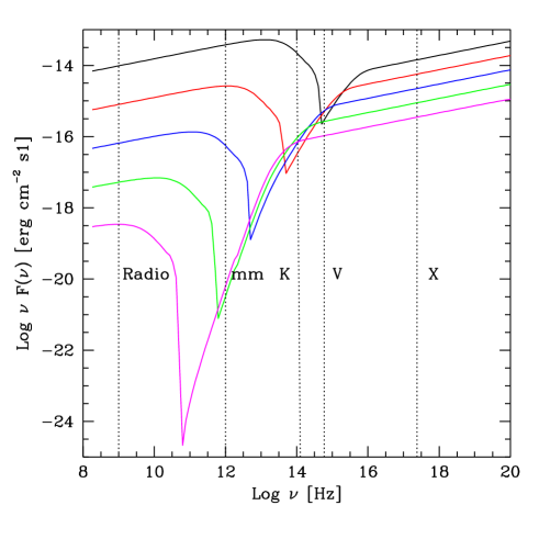
Figure 2: SEDs calculated according to the paramenters listed in Tab. 1. From top to bottom: $r$=20, 53, 140, 370 and 980 kpc. $\Gamma=4$ is assumed.

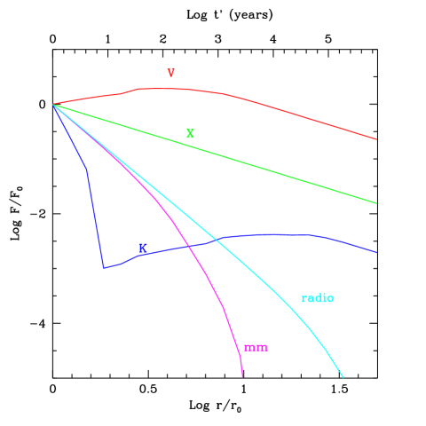
Figure 3: Flux profiles at different frequencies (5 GHz, 0.2 mm, $K$ band, $V$ band and 1 keV), calculated assuming the parameters listed in Table 1. $\Gamma=4$ is assumed. This is the case of the optical being made by inverse Compton off the CMB photons. In this case the optical will initially increase moving away from the knot in case A (bottom x–axis) or, alternatively (case B), it will initially increase in time (top x–axis, time is measured in the blob’s frame). See text for details on the two descriptions. The initial values of the fluxes at the different frequencies are: $F_{\rm 5\leavevmode\nobreak\ GHz}$= 209 mJy, $F_{\rm 0.2\leavevmode\nobreak\ mm}$= 4 mJy, $F_{K}=20$ $\mu$Jy, $F_{V}=0.1$ $\mu$Jy, $F_{\rm 1\leavevmode\nobreak\ keV}$=6.2 nJy.

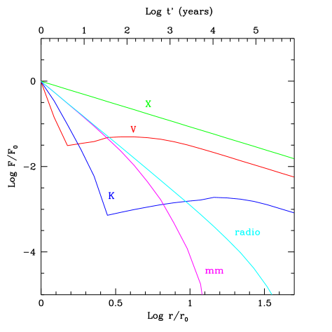
Figure 4: Flux profiles at different frequencies, assuming the parameters reported in Table 1. $\Gamma=4$ is assumed. This is the case of the optical being made by synchrotron. The initial values of the fluxes at the different frequencies are the same as in Fig. 3, except for the optical flux, now being $F_{V}$=2 $\mu$Jy.

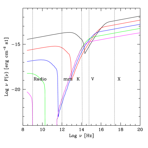
Figure 5: SEDs calculated according to the paramenters listed in Tab. 1. From top to bottom: $r$=20, 53, 140, 370 and 980 kpc. $\Gamma=15$ is assumed.

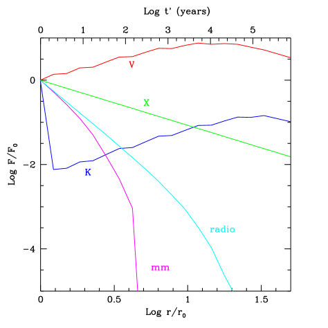
Figure 6: Flux profiles at different frequencies (0.2 mm, 5 GHz, $K$ band, $V$ band and 1 keV), for $\Gamma=15$, calculated assuming the parameters listed in Tab. 1. The optical emission is due to IC off the CMB. See that also in this case (as in Fig. 3) the optical will initially increase moving away from the knot in case A (bottom x–axis) or, alternatively (case B), it will initially increase in time (top x–axis, time is measured in the blob’s frame). See text for details on the two descriptions. The initial values of the fluxes at the different frequencies are: $F_{\rm 5\leavevmode\nobreak\ GHz}$= 93 mJy, $F_{\rm 0.2\leavevmode\nobreak\ mm}$= 1.7 mJy, $F_{K}=3$ $\mu$Jy, $F_{V}=0.13$ $\mu$Jy, $F_{\rm 1\leavevmode\nobreak\ keV}$=208 nJy.

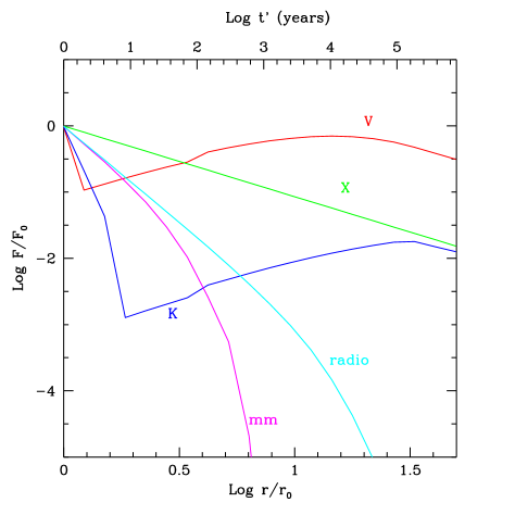
Figure 7: Flux profiles at different frequencies, for $\Gamma=15$, assuming the parameters reported in Table 1. This is the case of the optical being made by synchrotron. The initial values of the fluxes at the different frequencies are the same as in Fig. 6 except for the optical flux, now being $F_{V}$=1.5 $\mu$Jy.

2.2 Results

Using Eq. (5) we have computed the evolution of the spectral energy distributions (SED) as a function of $r$, assuming that $N(\gamma_{0},r_{0})$ is a power law between $\gamma_{\rm min,0}$ and $\gamma_{\rm max,0}$. The initial parameters, listed in Tab. 1, have been chosen to roughly match those found by fitting the SED of a knot of a large scale jet visible in radio, optical and X–rays. Note that the magnetic field does not affect the particle evolution (since we have assumed that the radiation energy density of the CMB dominates the cooling), but it determines the amount of the emitted synchrotron radiation. We have assumed that the magnetic field scales as $r^{-1}$ (as in the case in which the magnetic field has a prevalent toroidal component or in the case of constant magnetic flux along the jet). We have then assumed that the total number of electrons in a “slice” of the jet of width $\Delta r$ is conserved, and to calculate the emitted flux we have assumed a fixed width $\Delta r$. We have then consistently set the adiabatic constant $A=2/3$, corresponding to 2D expansion.

$r_{0}$	$B_{0}$	$A$	$\gamma_{\rm min,0}$	$\gamma_{\rm max,0}$	$\Gamma$	$\delta$	$z$	Fig.
kpc	$\mu$G
20	36	2/3	10	1e8	15	5.4	0.72	1
20	36	2/3	10	2.4e5	4	6	1	2, 3
20	36	2/3	10	5e5	4	6	1	4
20	10	2/3	10	2.4e5	15	9	1	5, 6
20	10	2/3	10	5e5	15	9	1	7
0.16	10	1	20	1e6	15	15	1	8, 9

Table 1: Input parameters for the examples shown in Fig. 1–9. In all cases we assumed $r_{\rm max}=20r_{0}$ and $N(\gamma)\propto\gamma^{-n}$ with $n=2.6$.

Having computed the SEDs in this way, we have constructed the flux profiles at different frequencies. Jets with a bulk Lorentz factor of $\Gamma=4$ and $\Gamma=15$ have been considered, since this is the range of values found when fitting quasars with large scale X–ray jets (Tavecchio et al. 2000; Sambruna et al. 2002; Celotti et al. 2001). Furthemore we have performed our calculations assuming that the optical flux is produced by the initial tail of the IC process (SEDs in Fig. 2 and Fig. 5; profiles in Fig. 3 and Fig. 6.) or by the high energy tail of the synchrotron process (profiles shown in Fig. 4 and Fig. 7). The only input parameter changing between the two sets of figures is the value of $\gamma_{\rm max,0}$.

In Fig. 2 we show the computed SEDs (for the case of $\Gamma=4$) assuming that the optical emission, at the starting point $r_{0}$, is due to initial part of the inverse Compton scattering off the CMB photons. Therefore the electrons producing this radiation have a small energy, and their cooling time is long. In this case the inverse Compton spectra are dominating the bolometric luminosity (this is also true at early times, although this may not be immediately clear from Fig. 2 which cuts the Compton spectrum before its peak), but not by a large factor at the beginning. At late times (or at some distance from $r_{0}$) the Compton dominance increases, since the magnetic field is assumed to decrease as $r^{-1}$, while the energy density of the CMB is constant. Fig. 3 shows the expected profiles of the flux in different bands using the same parameters used to construct the SEDs as shown in Fig. 2 and listed in Table 1. The x–axis of this figure can be expressed as a distance from the starting point (bottom axis) or equivalently as the time elapsed from the beginning of our calculations (top axis). In the latter case the light curves shown do not take into account light travel time effects: since the source is very extended, we will receive light from different evolutionary phases of the source (evolved from the near part, younger from the far part of the source). This is important of course for $t<r_{0}/c$: at these times the observed light curve is not the one shown in Fig. 3 (and the analogous Figs. 4, 6 and 7), but should be calculated (as e.g. in Chiaberge & Ghisellini 1999) considering the different travel paths of light rays produced in different parts of the source. For the purposes of the present paper these effects are not crucial, but they will be properly considered in our future studies. Note that if the profiles (i.e. bottom x–axis) shown in Fig. 3 correspond to emission from a standing shock (see below), and so a quasi–stationary case, then light travel time effects are not important, and Fig. 3 (and the other analogous figures) already fully describes the expected behavior.

Fig. 4 shows the profiles assuming that the optical emission is due to the high–energy tail of the synchrotron component. The only parameter different from those adopted for Fig. 2 and Fig. 3 is $\gamma_{\rm max,0}$, which is now slightly smaller (see Tab. 1).

Fig. 5 shows, by contrast, the SEDs predicted in the case of $\Gamma=15$. We have assumed that in this case the Compton emission is more dominant than in the previous case, due to the increased energy density of the CMB as seen in the comoving frame ($\propto\Gamma^{2}$). The other input parameters are listed in Table 1. Note that since the comoving CMB energy density is larger than in the previous case, the corresponding radiative cooling times are shorter, making the evolution of the high energy electrons faster, as can be seen comparing the radio and far IR spectra in Fig. 5 and Fig. 2 for late times (or for large distances). As in Fig. 2, the SEDs shown in Fig. 5 correspond to the case of the optical emission produced by the initial part of the inverse Compton radiation. Fig. 6 shows the corresponding profiles of the flux at different frequencies, while Fig. 7 shows the profiles assuming that, at the start, the optical flux is due to the tail of the synchrotron emission. Fig. 5 shows also that the synchrotron and IC emission components becomes “detached” at late times, when only the low energy electrons survive.

On inspecting the figures showing the flux profiles, a general trend emerges: the synchrotron produced fluxes are dimming faster than the IC/CMB ones, due to i) the different electron energies involved and ii) the decreasing magnetic field. In all cases the X–ray fluxes are roughly linearly decreasing with the distance $r$, while the initial decrease of the fluxes produced by the synchrotron process (away from the cutoffs) scale roughly as $r^{-3}$. As discussed below, this different behavior will be crucial when comparing our results with already existing data.

As mentioned in the Introduction, there are two possible cases for interpreting the results shown in Figs. 3, 4 and in Figs. 6, 7. Let us call them:

case A: streaming of particles from a stationary (in the observer frame) shock (bottom x–axis, distance from the acceleration site);

case B: rigidly moving blob whose internal particles have been accelerated at $r_{0}$ (top x–axis, time from the acceleration event in the blob reference frame).

If we are in case A (standing shock), then Figs. 3, 4, 6 and 7 directly show the profiles that would be observed in deep images of the jet for $r>r_{0}$ (assuming that the standing shock lives for a sufficiently long time to allow particles to move from $r_{0}$ to $r$). In the case of Fig. 3 and Fig. 6 for which the optical flux is due to the low–energy tail of the IC component, the optical flux increases with $r$. This happens despite the decrease in the normalization of $N(\gamma)$, and it is due to the fact that the optical is produced by the initial tail of the Compton emission (steeply rising with frequency), which increases its flux because of the decrease of $\gamma_{\rm min}$. In other words, in this case the overall spectrum shifts to lower frequencies and to lower fluxes: in the power law part of the spectrum the flux density decreases, while at the low energy end the flux density increases. In fact, when the optical flux is due to the power law part of the external Compton spectrum (for $r/r_{0}>10$), it decreases as the X–ray flux.

In case B (evolving blob), the particle distribution at a given $r$ is not directly related to the bright knots we are detecting, but is instead the “fossil” distribution of other unknown, acceleration phases occurred in the past (at $t^{\prime}=t^{\prime}_{0}$ on the top x–axis). Assuming then that there have been such phases in the past, with the optical flux initially produced through IC (Fig. 3 and Fig. 6), we should observe some bright optical knots with relatively weak X–ray and radio fluxes (with respect to the HST/Chandra bright knots). Knots which are bright only in the optical band have not been detected, and this could lead to the conclusion that the optical emission is always due to the high energy tail of the synchrotron spectra, and therefore to very high energy electrons. However, as will be discussed below, this conclusion is premature, since there may be an alternative possibility, in which the knot emission is considered as the result of the contribution of many sub–knot emission sites.

3 Comparison with observations

The results of the analysis described above can be compared with real profiles of nearby jets. One of the sources with the best published data is the luminous jet of 3C 273 (Sambruna et al. 2001; Marshall et al. 2001)

The jet presents numerous knots visible in radio, optical and X–rays. Sambruna et al. (2001) and Marshall et al. (2001) reach different conclusions about the viability of a synchrotron interpretation for the X–ray emission in knots A and B1 (the two most luminous portions of the jet). This is due to the different slopes of the optical spectrum derived by the two groups: Sambruna et al. (2001) present an optical spectrum with a slope systematically steeper than that of Marshall et al. (2001). For this reason Sambruna et al. can easily rule out the possibility that a unique spectral component from radio to X–rays can account from the overall spectrum, while the opposite conclusion is preferred by Marshall et al.

Despite this disagreement, both groups agree on the fact that the optical flux is due to synchrotron, and on the fact that maps at different frequencies yield knots of the same dimensions, and similar flux profiles. In other words, there appears to be no frequency–dependence of the size of knots.

However, according to the analysis given above, we would expect to find the radio knots to be larger than the optical ones, due to the longer lifetime of the radio-emitting electrons. An even larger region is expected in the case of X–ray knots produced by the IC process (i.e. by very low–energy electrons). Contrary to this expectation, it appears that knots have almost the same size at different frequencies.

In the following we examine what at first sight can be the possible and most plausible solutions:

• Consider a small and single standing shock. Suppose that the acceleration site is very compact, much smaller than the cross sectional radius of the jet, i.e. smaller than one arcsec. The angular resolution of Chandra in this case is not enough to resolve it in X–rays. In this way the adiabatic losses are much more effective. They corresponds to take, as $r_{0}$ in our figure, a region which is much less than a kpc (say a factor 10 less). In this case there are enough “doubling radii” to let adiabatic losses to decrease the flux (as in our figures). But the angular resolution of HST allows to resolve the emission region in the optical, and show that it cannot be smaller than about 1 arcsec. This implies that the acceleration site is extended (at least 1 arcsec), or made by several sub–units, contrary to our assumption.

• Consider moving blobs. In this case we see a snapshot of the blobs which are now active, and moving. The emission at different frequencies can in this case be cospatial, with no emission between the knots. The knots are observed to be active simultaneously according to our (observing) time, implying that they have been lighted up at different intrinsic times (because of light travel time effects). If these knots were the only existing ones, this requires a strong fine tuning. On the other hand, if the jet has many knots that randomly (in time and in location) light up, we always have the possibility to observe a few of them “on” (thus avoiding the fine tuning problem), but automatically this requires the existence of many “fossils” of previous active phases, emitting some X–rays, some radio, and no optical [i.e. with only the low energy part of $N(\gamma)$ surviving]. Since we observe no “fossil” knot, we disfavor this possibility. Yet another alternative is to assume that the jet really has only a few knots, which are always active. In this case we do not observe fossils, but we require that the particles in each knot are continuously reaccelerated. However this leads to another problem: in fact if the same particles are continuously reaccelerated, they should reach a typical energy (at which the cooling and acceleration timescales are equal), causing a pile–up at some energy, which is not observed. A possible way out is to assume that particles are only episodically reaccelerated, but this would require a strong fine–tuning between the duty cycle of the acceleration episodes and the cooling time of the optical electrons (the two times must be comparable).

We conclude that simple alternatives to the basic scenario (basic in the sense of a single homogeneous region emitting by synchrotron and external Compton) do not work or require fine–tuning. We are then forced to explore a slightly more complex alternative. In the next section we will then consider the possibility of knots composed of several sub–units (which we may identify as the acceleration sites), in order to make expansion losses more effective.

4 The clumping scenario

Assume that the knot is not homogenous, but is instead formed by several smaller substructures, i.e. several clumps. The key point of this idea is that small clumps can expand much more than a unique knot and therefore adiabatic losses can play a more important role than in the homogeneous case discussed above.

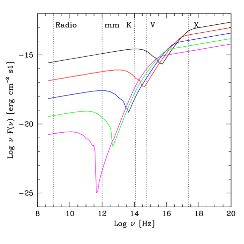
Figure 8: SEDs calculated in the “mini–knots” scenario, using the paramenters listed in Tab. 1. This illustrates the spectral evolution of a single mini–knot, for different expansion stages. From top to bottom: $r=$0.16, 0.28, 0.5, 0.9 and 1.6 kpc. Note that for this case we assumed a 3D expansion, and correspondingly used $A=1$.

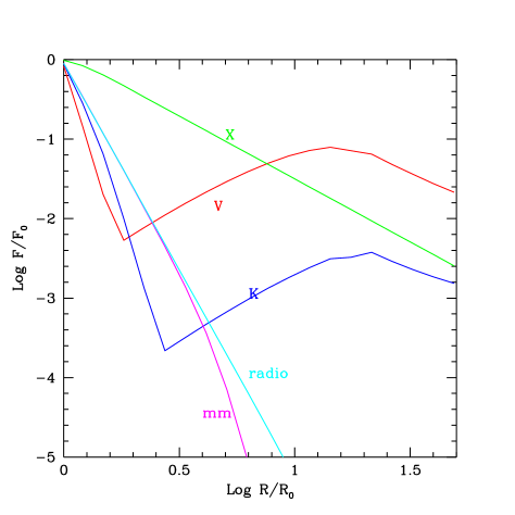
Figure 9: Flux profiles at different frequencies (0.2 mm, 5 GHz, $K$ band, $V$ band and 1 keV), for $\Gamma=15$, in the case of a single mini–knot, using the same parameters as in Fig. 8.

Assume then several acceleration sites which are much smaller than the transverse dimension of the jet. Let us call them “mini–knots”. Assume a number $N$ of mini–knots, and for simplicity assume that all of them are the same, with the same density $n_{i}$, radius $R_{i}$, volume $V_{i}$ and bulk Lorentz factor $\Gamma_{i}$. The filling factor of the mini–knots is $f\equiv NV_{i}/V$ where $V$ is the volume of the large knot. $R_{i}$ is limited to be smaller than – say – one tenth of the total size of the knot (to have enough expansion losses within the big knot). With these assumptions also the magnetic field $B_{i}$ must be the same, whatever the radius and number of mini–knots. This follows from the fact that in each mini–knot the magnetic field to CMB energy density ratio must be equal to the one-zone case, since the resulting spectrum must have the same synchrotron to IC luminosity ratio. Since $U_{\rm rad}$ in the mini-knot scenario is equal to the the one-zone scenario (as long as $\Gamma_{i}$ is the same), also the magnetic field must assume the same value in both scenarios.

Just for illustrative purposes, let us compare the case of a single homogeneous model in which the size of the emitting region is the entire big knot (we may call it the one–zone case: this is the case discussed up to now in the literature) with the clumping case. Assume for simplicity that the total number of emitting particles is the same in the two cases, as well as the magnetic field and the bulk Lorentz factor. What varies is the density and the size of the mini–knots: $n_{i}$ must be a factor $f$ larger than in the one–zone case. With these assumptions, the average bulk kinetic power (dominated by the cold proton component) in the case of the mini–knots is the same as in the one–zone case: the total number of particles is the same, and the time needed for them to cross a section of the jet is the same in both scenarios.

There is no obvious lower limit to the size $R_{i}$ of the mini–knots, but it must be noted that (within our assumptions) for a fixed number $N$ of mini–knots, the smaller their size, the larger their density, and the larger the deviation from equipartition between particle and magnetic energy densities. This deviation scales as the ratio of the particle density in each mini–knot and the density in the one–zone case, and therefore it scales as $f$. Therefore it is possible to have many (and small) mini–knots with a small filling factor, but this implies a large deviation from equipartition.

With respect to the one–zone case, each mini–knot has an enhanced particle pressure, and it is thus likely that it is overpressured with respect to its surroundings, implying expansion.

In conclusion, we propose that there are several mini–knots within the larger blob, which are the sites of particle acceleration, which are denser and hotter than the surroundings, leading automatically to the expansion of the entire mini–knot. What we see is then the convolution of the radiation produced by several expanding mini–knots.

The formation mechanisms of these “mini–knots” is outside the main goal of this paper; here we would only like to mention possible instabilities, clouds (filaments) crossing the jet (as proposed by, e.g., Blandford & Konigl 1979, although they considered this process at much smaller scales), or instabilities triggered by entrained gas that can act as an obstacle for the flow, forming mini–shocks. Another possibility is that particle acceleration is induced by reconnection events in the jet (e.g. Drenkhan & Spruit 2002). In this case the mini–knots could be identified as the reconnection sites.

If such mini–knots exist, then the problem to let low energy electrons adiabatically cool before they reach the borders of the bigger knot as detected by Chandra is solved. To illustrate this, we show in Fig. 8 the SEDs corresponding to a single mini–knot and in Fig. 9 the corresponding flux profiles at different frequencies. Since $r_{0}$ is much smaller than in the previous cases, all the timescales are shorter, changing the relative importance of the radiative and adiabatic losses. Note that, in Fig. 9, the entire range of the x–axis is now 1 arcsec, as opposed to 10 arcsec of the previous ones (for a source at $z\sim 1$).

While cooling for radiative and adiabatic losses, and while the mini–knot expands, the electrons emit some radiation even outside the acceleration sites. High energy particles, producing the optical synchrotron radiation, are the ones cooling the most, making the optical flux to decrease at the faster rate initially. Then, when $\gamma_{\rm min}$ is low enough to produce optical radiation by the inverse Compton process with the CMB photons, we have an increasing optical flux (until it is produced by the rising initial tail of the IC spectrum). The same situation occurs (but later) for the infrared flux. The X–ray flux instead steadily decreases, being always produced by low energy electrons. In conclusion, having enough angular resolution, one should resolve each mini–knot, especially in the optical and infrared bands, where the contrast between the emission inside and outside the mini–knots is the largest. However, the flux between the knots never vanishes, and remains at a considerable level especially in the X–ray band.

Another point that must be considered is the nature of the medium between the “mini-knots”. If particle acceleration is concentrated in the “mini-knots”, the possibility that appears the most natural is that the medium is mainly composed by cold particles, perhaps embedded in a very low magnetic field. These particles would emit through IC/CMB: the emission is concentrated in the IR-optical regime, at $\sim 10^{14}$ Hz. In this case there would be the possibility that this material is detectable in a near future with NGST, apearing as a “diluting” emission between mini-knots. The possibility to detect the emission mainly depends on the density of the medium: even an upper limit could help to better characterize the density contrast between the clumps and the external medium.

5 Summary

We have discussed how the presence of low energy electrons in jets, predicted by the IC/CMB model, poses important problems related to their extremely long radiative cooling time. In fact we know that the X–ray emission (as well as the optical and radio emission) comes in localized regions of the jet (the knots), despite the fact that the X–ray emitting electrons cannot radiatively cool inside these small regions. This motivated the exploration of the possible effects of adiabatic losses that for low energy electrons are much more important than radiative losses. We have shown the predicted profiles at different frequencies under different assumptions.

In particular we have identified two possible cases: in case A we considered a standing (in the observer frame) shock, while in case B the emission we observe is produced in a moving blob. Some general consequences appropriate for future and more detailed observations will be briefly discussed below and in a forthcoming paper.

However, the existing observations already pose a problem. In fact comparing our results with the data of nearby aligned radio sources (i.e. nearby blazars, such as 3C 273), we found that in any case (A or B) radiative and adiabatic losses cannot explain what is observed. In case A we would expect radio (and perhaps X–ray) knots larger than the optical ones, contrary to what is observed. In case B we would expect a number of unobserved “fossil knots”, bright in the radio and especially in the X–ray bands, but much fainter in the optical.

A possible way out of this puzzle is to admit that the emitting region is clumped in several mini–knots, allowing particles to cool by adiabatic expansion much more than in the one–zone case. These clumps can originate from different processes. An important consequence of this scenario is that, since the magnetic field energy density has to be the same as in the case of the one-zone scenario, the emitting region is far from equipartition, with the particle energy density dominating over the magnetic one.

6 Discussion

In large scale jets, with moderate values of the energy densities involved (both magnetic and radiative), the radiative cooling times are very long for all but the TeV electrons responsible for the high energy tail of the synchrotron emission. In particular, in the IC/CMB models, the X–ray flux is produced by electrons with random Lorentz factors of the order of 10–100, implying that they never cool through radiation losses. Adiabatic losses must then play a crucial role to explain the knotty morphology of large scale X–ray/optical/radio jets.

What we see can be the result of particle acceleration occurring in two different scenarios: acceleration can occur either at the front of a standing shock or accelerated particles can be injected throughout a blob moving along with the jet.

In the first case we expect to observe an extension of the emission region downstream to the shock (at larger distances from the shock front), whose size depends on the observing frequency. In particular, since X–rays are produced by low-energy electrons, the size of the X–ray emitting region must be larger than the radio one. The optical behavior is more complex, being due initially to the highest energy and rapidly cooling electrons, and later being due to the lowest energy electrons through IC.

In the moving blob case, particles are confined and evolve within the blob, and the particle evolution translates into a time dependent appearance of the blob itself. In particular, also old, “fossil” blobs are expected to be observable, bright especially in the X–ray band, relatively less in the radio and optical. Even taking into account adiabatic losses, the lifetime of the X–ray emission is long (compared to $R/c$, where $R$ is the size of the blob), and therefore the number of these “fossil blobs” should be larger than the young ones.

These considerations point towards the possibility to discriminate between the two scenarios: observing ”X–ray trails” more elongated than the radio and the optical ones would favor the standing shock scenario, while observing isolated X–ray knots (with weaker radio and optical emission, but cospatial) would favor the moving blob scenario. In order to perform such discriminating observations one needs sub–arcsec angular resolution at flux levels of the order of $10^{-15}$ erg cm^-2 s^-1 or better, at least in the optical/IR, possibly in the mm and radio domains. In general, NGST, LBT and ALMA are then required.

Nearby blazars can already give some indications, since for them HST already can probe the interesting spatial scales. We have compared our results with the existing data of 3C 273. What we found is at first sight puzzling, since the flux outside the knots decreases fast and no “fossils” are observed. We have then proposed that what appears a single knot is instead the convolution of several smaller emission sites. This allows particles to adiabatically cool within the observed knot, allowing the flux to decrease fast outside it.

A natural consequence of this clumping scenario is that the emission can be variable on short (months–years) timescales. We note that, very recently, the knot HST–1 in M87 (emitting by synchrotron from the radio to the X–ray band), has been claimed to vary on a timescale of months in the X–ray and optical bands, and not in the radio (Harris et al. 2002). These variations have been attributed to the radiative cooling of the synchrotron emitting electrons. However, the dimension of knot HST–1 is of the order of $\sim 100$ pc, implying a minimum observable variability timescale of $\sim$300 years, corresponding to the light crossing time. If the HST–1 blob is instead composed of several mini–knots, the minimum variability timescale becomes the light crossing time of each single mini–knot (as long as the total number of mini–knots is not large, otherwise the amplitude of variability is diluted and becomes unobservable). Also in M87’ – suggest rewriting this sentence as follows ‘M87, then, also shows some evidence for clumped substructure in the jet knots, as we have suggested in the case of 3C273 using a completely independent argument.

- (1) Blandford R.D., & Konigl A., 1979, ApJ, 232, 34
- (2) Celotti A., Ghisellini G. & Chiaberge M., 2001, MNRAS, 321, L1
- (3) Chiaberge M. & Ghisellini G., 1999, MNRAS, 306, 551
- (4) Chartas G., Worrall D.M., Birkinshaw M., et al., 2000, ApJ, 542, 655
- (5) Drenkhahn, G. & Spruit, H. C. 2002, A&A, 391, 1141
- (6) Ghisellini G. & Celotti A., 2001, MNRAS, 327, 739
- (7) Hardcastle M.J., Worrall D.M., Birkinshaw M., Laing R.A. & Bridle A.H., 2002, MNRAS, 334, 182
- (8) Hardcastle M.J., Birkinshaw M. & Worrall D.M., 2001, MNRAS, 326, 1499
- (9) Harris D.E. & Krawczynski H., 2002, ApJ, 565, 244
- (10) Harris D.E. et al, 2002, in ”The physics of relativistic jets in the Chandra and XMM era”, New Astronomy Review, Eds. G. Brunetti, D.E. Harris, R.M. Sambruna & G. Setti, in press
- (11) Kraft R.P., Forman W.R., Jones C., Murray S.S., Hardcastle M.J. & Worrall D.M., 2002, ApJ, 569, 54
- (12) Malesani D., 2002, unpublished thesis, Milano University.
- (13) Marshall H.L., Harris D.E., Grimest J.P. et al., 2001, ApJ, 549, L167
- (14) Pesce J.E., Sambruna R.M., Tavecchio F. et al., 2001, ApJ, 556, L79
- (15) Sambruna R.M., Maraschi L., Tavecchio F. et al., 2002, ApJ, 571, 206
- (16) Sambruna R.M., Urry C.M., Tavecchio F. et al., 2001, ApJ, 549, L161
- (17) Schwartz D.A., 2002, ApJ, 571, L71
- (18) Schwartz D.A., Marshall H.L., Lovell J.E.J., et al., 2000, ApJ, 540, L69
- (19) Siemiginowska A., Bechtold J., Aldcroft T.L., Elvis M., Harris D.E. & Dobrzycki A., 2002, ApJ, 570, 543
- (20) Sikora M., Blazejowski M., Begelman M.C. & Moderski R., 2001, ApJ, 554, 1
- (21) Tavecchio F., Maraschi L., Sambruna R.M. & Urry C.M., 2000, ApJ, 544, L23
- (22) Wilson A.S. & Yang Y., 2002, ApJ, 568, 133
- (23) Wilson A.S., Young A.J., & Shopbell P.L., 2001, ApJ, 547, 740