Modeling Fluctuations in the GRB-Afterglow Light Curves

Abstract

The fluctuations observed in the light curves of some GRB-afterglows (such as GRB 021004) provide a useful tool to probe the circum-burst density profile and to probe the variations in the energy of blast-wave with time. We present a general formalism that reduces the calculation of the observed light curve from a Blandford-Mackee blast-wave to the evaluation of a one dimensional integral. Using this formalism we obtain a simple approximation to the general light curve that arises in more complex situations where the afterglow’s energy or the external density vary. The solution is valid for spherically symmetric profiles and it takes a full consideration of the angular time delay effects. We present the light curves of several external density profiles and demonstrate the effects of density variations on the light curve. We also re-visit the afterglow of GRB021004 and we find that the steep decay after the first bump ($\sim 4000sec$) cannot result from a spherically symmetric density variation or from the passage of the synchrotron frequency through the optical band. This suggests that an angular structure is responsible to some of the observed features in the light curve. This may be the first evidence that an angular structure is important in the early stages of the afterglow.

1 Introduction

The basic theory of the multi wavelength afterglow which follows GRBs is well established. The afterglow emission is produced by an interaction between a relativistic expanding fireball and the circumburst material. This interaction produces a relativistic blast wave which heats the external medium and produces the observed emission. The dominant radiation process is most likely synchrotron.

After a short radiative phase the blast wave becomes adiabatic and the hydrodynamic profile behind the shock relaxes to a self-similar solution (Blanford & Mackee 1976 ; hereafter BM76). The observed synchrotron light curve from a Blanford-Mackee (BM) self similar shell is presented by Granot, Piran & Sari (1998) as a two dimensional nontrivial numerical integral. We use here the self similar properties of the BM solution to reduce the expression of Granot et. al. (1998) to a simple one dimensional integral. The integrand expresses the contribution of the instantaneous emission from a BM shell at a given radius. This simplification is important for two reasons. First, it allows an easy calculation of interesting physical quantities (e.g. the afterglow image, see Granot et. al. 1998) that had to be calculated numerically so far. Second, and more importantly, it enables us to obtain a good approximation of the observed afterglow when the external density and/or blast-wave energy varies, as long as the variations are spherically symmetric.

We use our solution to investigate several external density profiles. We find that due to angular smoothing, even a short length scale density variation, results in a fluctuation in the light curve of more than one order of magnitude in time. Second, we show that above the cooling frequency, a density enhancement results in a fluctuation with amplitude of less than 20% , while a density drop results in a larger fluctuation (a drop of one order of magnitude in the density results in a fluctuation of 40%).

Nakar, Piran & Granot (2002) investigated different possible explanations to the peculiar afterglow of GRB 021004. This unusual afterglow shows a clear deviations from a smooth temporal power law decay. A first bump is observed after $\sim 4000sec$, this bump is followed by a steep decay. Later the afterglow shows additional deviations from a power-law decay. Nakar et al. 2002 considered the angular effects only approximately. Here we re-visit this afterglow taking a full consideration of the angular effects. We show that the first bump and the steep decay that follows it, cannot result from spherically symmetric density variations. We show also that the fast decay is inconsistent with a simple transition of the typical synchrotron frequency, $\nu_{m}$, through the optical band (with a constant ISM density profile). Although passage of $\nu_{m}$ is consistent with the timing and with the rising phase of the bump (Kobayashi & Zhang 2002), the fast decay requires another mechanism (most likely an angular dependent one). These results suggests that an angular structure is important in the early afterglow of GRB 021004.

In §2 we present our solution. In §3 we consider the effects of density and energy variations. In §4 we discuss the afterglow of GRB 021004 and at the last section we present our conclusions. The detailed calculations which lead to the solution we present at §2 are described in the appendix.

2 The Blandford-McKee light curve

We consider an adiabatic relativistic blast wave propagating into an external medium with a regular density profile $n_{ext}\propto r^{-k}$ ($k<3$). We calculate the observed flux from a slow cooling synchrotron. As commonly done (Sari, Piran & Narayan 1998) we assume that the energy of the magnetic field and the energy of the hot electrons, are constant fractions of the internal energy ($\varepsilon_{B}$ and $\varepsilon_{e}$ respectively) and that the hot electrons’ initial distribution is a power law with an energy index $p$. We express the solution as a simple one dimensional integral. This solution can be used to calculate different properties of the afterglow, or as an approximation to the observed afterglow in the cases of a variable external density and/or a variable blast-wave energy (see section 3).

The spectral shape of the observed flux is well approximated (Sari et al. 1998) by a broken power law with several power-law segments. In the slow cooling regime there are four segments separated by $\nu_{a},\nu_{m}$ and $\nu_{c}$: the self-absorption, synchrotron and cooling frequencies respectively. We discuss here only the emission above $\nu_{a}$. First we consider the solution when the observed frequency, $\nu$, is far from the break frequencies and later we address the solution near the break frequencies.

We distinguish between three relative frames. The center of the explosion and the observer at infinity are at rest at the source frame. We denote the time in the source frame by $t$ and we calibrate $t=0$ to the explosion time. The fluid frame is the rest frame of the fluid, we denote all variables in the fluid frame with a ’prime’. The observer frame is at rest compared to the source frame. However, the observer time is measured according to the arrival time of photons to the observer. We denote the observer time as $T$, and we calibrate $T=0$ to the arrival time of a photon emitted at $t=0$, $r=0$ ($r$ is the distance from the explosion).

We address first the problem of an instantaneous emission from a very thin shell located at a radius $r$ and propagating with a Lorentz factor $\gamma$ (this problem or related ones where considered by Fenimore, Madras & Nayakshin (1996), Kumar & Panaitescu 2000, Ioka & Nakamura 2001, Ryde & Petrosian 2002 and others). Due to the relativistic beaming the observer receives mainly photons emitted up to an angle of $\theta=1/\gamma$ relative to the line-of-sight. The observer time delay between two photons emitted simultaneously at a radius $r$, one on the line-of-sight and the other from $\theta=1/\gamma$ is $T_{ang}=r/2c\gamma^{2}$. Hence, an instantaneous emission in the source frame is observed as a finite pulse with a duration $\sim T_{ang}$. The observed time of the first photon (emitted on the line-of-sight) is $T_{los}=t-r/c$, where $t$ is the time in which the shell radiates in the source frame. Thus an instantaneous emission from a very thin shell produces a pulse that is observed for $T_{los}\leq T\leq T_{los}+T_{ang}$. The emission that arrives at larger $T$ is emitted at larger $\theta$. Fenimore et al. (1996) calculated the shape of the pulse for an intrinsic power law spectrum with a power law index $\beta$: $P_{\nu}\propto\nu^{\beta}$. They find that the observed flux at $T>T_{los}$ is:

$$F_{\nu}(T)\propto\nu^{\beta}\left(1+\frac{T-T_{los}}{T_{ang}}\right)^{-(2-\beta)}.$$ (1)

The observed flux, at an observer time $T$, from an arbitrary spherically symmetric emitting region is given by Granot et. al. (1998):

$$F_{\nu}(T)=\frac{1}{2D^{2}}\int_{0}^{\infty}dt\int_{0}^{\infty}r^{2}dr\int_{-1}^{1}d(cos\theta)\frac{n^{\prime}(r)P^{\prime}_{\nu}(\nu\Lambda,r)}{\Lambda^{2}}\delta(t-T-\frac{r\,\,cos\theta}{c}),$$ (2)

where $n^{\prime}$ is the emitters density and $P^{\prime}_{\nu}$ is the emitted spectral power per emitter, both are measured in the fluid frame; $\theta$ is the angle relative to the line of sight, and $\Lambda^{-1}=1/\gamma(1-v\,\,cos\theta/c)$ ($v$ is the emitting matter bulk velocity) is the blue-shift factor. Below we calculate this expression for an instantaneous emission from a shell with a Blandford-Mackee (BM) self-similar profile. The BM self similar shell has a width of, $\Delta R\approx R/2(4-k)\Gamma^{2}$, where $R$ and $\Gamma$ are the shock’s radius and Lorentz factor respectively. BM76 show that all the variables behind the relativistic blast-wave are functions only of the dimensionless parameter, $\chi=[1+2(4-k)\Gamma^{2}](1-r/ct)$. $\chi=1$ at the shock front and it increases with the distance (down stream) from the shock.

We will calculate $F_{\nu}(T)$ by integrating over the contributions from BM shells (Eq. 3 below) at different radii. To do so we calculate the contribution to the observed flux at time $T$ of the emission emitted by the blast wave during the time that the shock propagates from the radius $R$ to $R+dR$. We denote this contribution as $A_{\nu}(R)\cdot g_{\beta}(R,T,k)dR$ where $\beta$ is the spectral index in the relevant power-law segment. $A_{\nu}(R)dR$ is the emitted spectral power during the time that the shell propagates from $R$ to $R+dR$. The function, $A_{\nu}$, includes only numerical parameters which remain after the integration over $r$ and $cos\theta$ in Eq. 2 and it depends only on the conditions of the shock front along the line-of-sight. The second factor $g_{\beta}$ is a dimensionless factor that describes the observed pulse shape of an instantaneous emission. $g_{\beta}$ is obtained by integration over $cos\theta$ and $r$ in Eq. 2 and it includes only the radial and angular structure of the shell. The self-similar profile of the shell enables us to express $g_{\beta}$ as a general function that depends only on the dimensionless parameter $\widetilde{T}=\widetilde{T}(R,T)$ (which we define later), hence $g_{\beta}(R,T,k)=g_{\beta}(\widetilde{T},k)$. The function $g_{\beta}(\widetilde{T},k)$ is calculated only once for a given ${\beta}$ and external density profile.

Using the self similar profile of the emitting region and neglecting terms up to the lowest order of $O(\gamma^{-2})$ (the detailed derivation is described in details in the Appendix), we reduce Eq. 2 to:

$$F_{\nu}(T)=\frac{1}{D^{2}}\int_{0}^{R_{max}}A_{\nu}(R)g_{\beta}(\widetilde{T},k)dR,$$ (3)

where $R_{max}$ satisfies :

$$T_{los}(R_{max})=T,$$ (4)

and $D$ is the distance to the source (cosmological factors are not considered through the paper). When all the significant emission from the shell at radius $R$ is within the same power-law segment, $\beta$, (i.e $\nu$ is far from the break frequencies) then $A_{\nu}$ and $g_{\beta}$ are given by:

$$A_{\nu}(R)=H_{\nu}\left\{\begin{array}[]{c}R^{2}\,n^{4/3}_{ext,0}\,E_{52}^{1/3}\,M_{29}^{-1/3}\quad\nu<\nu_{m}\\ R^{2}\,n^{(5+p)/4}_{ext,0}\,E_{52}^{p}\,M_{29}^{-p}\quad\nu_{m}<\nu<\nu_{c}\\ R\,n^{(2+p)/4}_{ext,0}\,E_{52}^{p}\,M_{29}^{-p}\quad\nu>\nu_{c}\end{array}\right.\frac{erg}{sec\cdot cm\cdot Hz},$$ (5)

where $R$ is the radius of the shock front, $n_{ext}(R)$ is the external density, $E$ is energy in the blast-wave, $M(R)$ the total collected mass up to radius $R$ and $H_{\nu}$ is a numerical factor which depends on the observed power law segment (see Eq. 14). We denote by $Q_{x}$ as the value of the quantity $Q$ in units of $10^{x}$ (c.g.s).

$$g(\widetilde{T},\beta,k)=\left\{\begin{array}[]{c}\frac{2}{(4-k)}\int^{1+2(4-k)\widetilde{T}}_{1}\chi^{-\mu(\beta,k)}\left(1-\frac{1}{2(4-k)}+\frac{2(4-k)\widetilde{T}+1}{2(4-k)\chi}\right)^{-(2-\beta)}d\chi\quad\nu<\nu_{c}\\ (1+\widetilde{T})^{-(2-\beta)}\quad\nu>\nu_{c}\end{array}\right.,$$ (6)

where

$$\widetilde{T}(R,T)=\frac{(T-T_{los}(R))}{T_{ang}(R)},$$ (7)

and

$$\mu(\beta,k)\equiv 3\cdot(71-17k)/(72-18k)-\beta\cdot(37+k)/(24-6k).$$ (8)

This set of equations is completed with the following relations between the different variables of the blast wave, the observer time and the break frequencies:

$$\nu_{m}=5\cdot 10^{12}n^{1/2}_{ext,0}E^{2}_{52}M^{-2}_{29}\varepsilon^{1/2}_{B-2}\varepsilon_{e-1}^{2}\>Hz,$$ (9)

$$\nu_{c}=2.5\cdot 10^{17}R_{17}^{-2}n_{ext,0}^{-3/2}\varepsilon^{-3/2}_{B-2}\>Hz,$$ (10)

$$M(R)\equiv 4\pi m_{p}\int^{R}_{0}r^{2}n(r)dr\>\left(=\frac{4\pi n_{*}m_{p}}{3-k}R^{3-k}\right),$$ (11)

$$T_{los}(R)=\frac{c}{4}\int^{R}_{0}\frac{M(r)}{E(r)}dr\>\left(=\frac{\pi cn_{*}m_{p}}{(4-k)(3-k)E}R^{4-k}\right),$$ (12)

$$T_{ang}(R)=\frac{cRM(R)}{2E(R)}\>\left(=2(4-k)T_{los}(R)\right),$$ (13)

where $m_{p}$ is the proton mass and the values in the parenthesis are for a constant energy and a density profile of $n_{ext}=n_{*}r^{-k}$ ($k<3$). The numerical coefficient of Eq. 5, $H_{\nu}$, is given by:

$$H_{\nu=}\left\{\begin{array}[]{c}9\cdot 10^{-26}\,\varepsilon^{2/3}_{e-1}\,\varepsilon^{1/3}_{B-2}\,\nu^{1/3}\quad\nu<\nu_{m}\\ 2\cdot 10^{-21}(5\cdot 10^{12})^{(p-1)/2}\,\varepsilon^{p-1}_{e-1}\,\varepsilon^{(p+1)/4}_{B-2}\,\nu^{(1-p)/2}\quad\nu_{m}<\nu<\nu_{c}\\ \frac{3p+6}{3p+2}6\cdot 10^{-3}(2.5\cdot 10^{6})^{p}\,\varepsilon^{p-1}_{e-1}\,\varepsilon^{(p-2)/4}_{B-2}\,\nu^{-p/2}\quad\nu>\nu_{c}\end{array}\right..$$ (14)

For the two canonical cases of ISM ($n_{ext}=n_{*}$, $k=0$) and wind ($n_{ext}=n_{*}r^{-k}$; $k=2$) Eq. 5 is reduced to:

$$A_{\nu,los}(R)=H_{\nu}\left\{\begin{array}[]{c}2\cdot 10^{34}R_{17}\,n_{*,0}\,E_{52}^{1/3}\quad\nu<\nu_{m}\\ (0.07)^{-p}\cdot 10^{34}R_{17}^{2-3p}\,n^{(5-3p)/4}_{*,0}\,E_{52}^{p}\quad\nu_{m}<\nu<\nu_{c}\\ (0.07)^{-p}\cdot 10^{17}R_{17}^{1-3p}\,n^{(2-3p)/4}_{*,0}\,E_{52}^{p}\quad\nu>\nu_{c}\end{array}\right.\frac{erg}{sec\cdot cm\cdot Hz}\;ISM,$$ (15)

$$A_{\nu,los}(R)=H_{\nu}\left\{\begin{array}[]{c}2\cdot 10^{34}R^{5/3}_{17}\,n_{*,34}\,E_{52}^{1/3}\quad\nu<\nu_{m}\\ (0.2)^{-p}\cdot 10^{34}R_{17}^{2-p}\,n^{(5-3p)/4}_{*,34}\,E_{52}^{p}\quad\nu_{m}<\nu<\nu_{c}\\ (0.2)^{-p}\cdot 10^{17}R_{17}^{1-p}\,n^{(2-3p)/4}_{*,34}\,E_{52}^{p}\quad\nu>\nu_{c}\end{array}\right.\frac{erg}{sec\cdot cm\cdot Hz}\;WIND,$$ (16)

For ${\nu}>{\nu}_{c}$ the expression of $g_{\beta}(\widetilde{T},k)$ in Eq. 6 is analytic. We can obtain an approximated analytic expression also for the spectral segment $\nu_{m}<\nu<\nu_{c}$. The rise time of the pulse is very short ($g_{\beta}$ reaches half of its maximal value at $\widetilde{T}\approx 0.02$, and its maximal value at $\widetilde{T}\approx 0.14$). Hence, for $\widetilde{T}<0.25$ we can approximate $g_{\beta}$ as a constant. For $\widetilde{T}>0.25$ the width of the BM shell is negligible and we can approximate the pulse decay as an emission from a thin shell with an effective angular time, $T_{ang}^{eff}$. We calculate $T_{ang}^{eff}$ by approximating the BM profile as a series of thin shells whose Lorentz factors that vary with $\chi$, emitting at the same time an radius . Due to the different Lorentz factors each shell has its own angular time ($T_{ang}(\chi)\propto\chi$). The effective angular time is a weighted average of $T_{ang}(\chi)$. The weights are the emitted spectral power density at $\chi$: $\propto\chi^{-\mu(\beta,k)}$ (see the appendix for details). Hence: of the

$$g_{\beta}(\widetilde{T},k)\approx\left\{\begin{array}[]{c}g_{\beta}(0.25,k)\quad\widetilde{T}<0.25\\ g_{\beta}(0.25,k)\left(\frac{1+\widetilde{T}(\mu-2)/(\mu-1)}{1+(\mu-2)/4(\mu-1)}\right)^{-(2-\beta)}\quad\widetilde{T}>0.25\end{array}\right.\nu_{m}<\nu<\nu_{c},$$ (17)

$$T^{eff}_{ang}=\frac{\mu-1}{\mu-2}T_{ang}(R)\quad\nu_{m}<\nu<\nu_{c}.$$ (18)

The validity of this approximation is shown in Fig 1, which compares the approximation of Eq. 17 with the complete calculation of Eq. 6 and a full numerical simulation of the emission from a BM blast wave. The numerical simulations include both the adiabatic and the radiative cooling of the electrons.

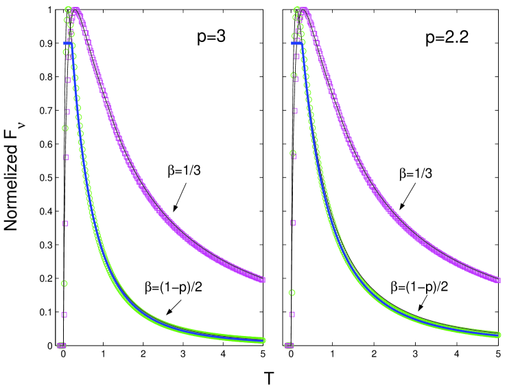
Figure 1: .The general pulse shape in ISM, $g_{\beta}(\widetilde{T},k=0)$, for electrons’ energy indices $p=2.2$ and $p=3$. The thin solid lines corresponds to Eq. 6, the thick lines are the results of Eq. 17, and the squares and the circles are the results of a full numerical simulation of the emission from a BM blast wave. Note that the approximation of Eq. 17 is very good during the decay of the pulse. It is almost impossible to distinguish between the approximation and the exact calculation of $g_{\beta}(\widetilde{T},k=0)$ at this phase. At $\widetilde{T}>10$, the approximation is less accurate, but at this stage the contribution of the pulse to the observed light curve is negligible. Similar results are obtained for other $k$ values.

2.1 The light curve in the vicinity of the break frequencies

The above solution is valid only when the observed frequency is far from any of the break frequencies ($\nu_{m}$ and $\nu_{c}$). To understand the behavior in the vicinity of the break frequencies we consider a thin shell with an intrinsic broken power-law spectrum. $\nu^{\prime}_{b}$ is the break frequency in the shell’s rest frame ($\beta=\beta_{1}$ for $\nu^{\prime}<\nu^{\prime}_{b}$ and $\beta=\beta_{2}$ for $\nu^{\prime}>\nu^{\prime}_{b}$). $\nu^{\prime}_{b}$ is constant along the shell; at the observer frame, however, the break frequency is $\nu_{b}=\nu^{\prime}_{b}/\Lambda$ ($\Lambda^{-1}$ is the blue-shift factor which defined after Eq. 2), which decrease with $\theta$. Hence, it is possible that at first the observed frequency, $\nu$, is smaller than $\nu_{b}$, while at later times it is larger than $\nu_{b}$. In other words at different times the observed frequency is within different power-law segments. In this case Eq. 1 is still valid, only $\beta=\beta_{1}$ for $\nu/\nu_{b}>(1+(T-T_{los})/T_{ang})$ and $\beta=\beta_{2}$ for $\nu/\nu_{b}<(1+(T-T_{los})/T_{ang})$.

When the instantaneous emission is from a BM shell then the blue-shift varies within different parts of the shell (larger $\chi$ and/or larger $\theta$ result in a smaller $\Lambda^{-1}$). Hence, the observed flux from an instantaneous BM shell at a given observer frequency at a given time results from emission in a range of fluid frame frequencies. Therefore, it is possible that the flux in a given observed frequency at a given time corresponds to different power-law segments at the emission from different parts of the shell.

For $\nu\ll\nu_{c}$ the observed emission arrives from the whole width of the shell. The integration over the parameter $\chi$ within the pulse shape, $g$, is both along the radial coordinate and the angular coordinate (larger $\chi$ is smaller $r$ and lower $\theta$). This integration depends on the spectral index $\beta$, which is different for $\nu<\nu_{m}$ ($\beta_{1}=1/3$) and $\nu>\nu_{m}$ ($\beta_{2}=(1-p)/2$). The transition from one spectral index to the other occur at some critical $\chi$ value, $\chi_{m}$, which satisfies:

$$\chi_{m}^{\xi}(1-\frac{1}{2(4-k)})+\chi_{m}^{\xi-1}(\widetilde{T}+\frac{1}{2(4-k)})-\frac{\nu_{m}}{\nu}=0$$ (19)

where $\xi=(37+k)/(24-6k)$. Here the pulse shape depends also on $\chi_{m}$ and it takes the form:

$$A_{\nu}g_{\beta_{1},\beta_{2}}(\widetilde{T},k,\chi_{m})=\frac{2}{(4-k)}\left[A_{\nu<\nu_{m}}\int^{\chi_{m}}_{1}\chi^{-\mu(\beta_{1},k)}\left(1-\frac{1-{\chi}^{-1}}{2(4-k)}+\frac{\widetilde{T}}{\chi}\right)^{-(2-\beta_{1})}d\chi\right.$$

$$\left.+A_{\nu>\nu_{m}}\int^{1+2(4-k)\widetilde{T}}_{\chi_{m}}\chi^{-\mu(\beta_{2},k)}\left(1-\frac{1-{\chi}^{-1}}{2(4-k)}+\frac{\widetilde{T}}{\chi}\right)^{-(2-\beta_{2})}d\chi\right]\quad\nu<\nu_{c}$$ (20)

The weight of the contribution of each power-law segment is given by the corresponding $A_{\nu}$. Whenever $\chi_{m}<1$ than the whole shell emits within the same power-law segment, $\nu>\nu_{m}$, and Eq. 20 is reduced to Eq. 6. Similarly, when $\chi_{m}>1+2(4-k)\widetilde{T}$ the whole shell emits within the power-law segment of $\nu<\nu_{m}$. Eq. 20 provides an exact solution of the spectral break at $\nu_{m}$ and an exact light curve break when $\nu_{m}$ passes through the observed frequency. Just like Eq. 6, $g_{\beta_{1},\beta_{2}}(\widetilde{T},k,\chi_{m})$ is calculated only once. However in this case it should be calculated for every $\widetilde{T}$ and $\chi_{m}$.

When $\nu\approx\nu_{c}$ the emission arrives only from a thin part at the front of the BM shell. The local spectrum of the emission in the fluid frame vary along the shell, and an exact solution should follow the exact profile of the local emission. Hence, there is no simple solution for the exact flux in the vicinity of $\nu_{c}$ (a full solution of the break shape in ISM and wind is presented at Granot & Sari 2001). A partial treatment of the break is obtained by taking a sharp transition from $\nu<\nu_{c}$ to $\nu>\nu_{c}$ when $\nu(1+\widetilde{T})=\nu_{c}$, i.e taking the part of $\nu<\nu_{c}$ at Eq. 6 for $\widetilde{T}<\nu_{c}/\nu-1$ and the part of $\nu>\nu_{c}$ for $\widetilde{T}>\nu_{c}/\nu-1$. In this approximation $g_{\beta_{2},\beta_{3}}(\widetilde{T},k)$ is discontinuous ($\beta_{3}=-p/2$), but the observed light curve and spectral break are rather smooth.

2.2 The emission from a collimated jet

So far we have dealt with a spherical symmetric systems. However, in GRBs the relativistic outflow is most likely collimated into narrow jets with an opening angle $\theta_{j}$. Our solution is not valid if the hydrodynamical parameters depend on the angle from the jet axis. But if they do not, then we can easily generalize our results to a jet as long as the observation angle relative to the jet axis is much smaller than $\theta_{j}$. In this case the emission from the edges of the jet at a given $R$ is observed at $\widetilde{T_{j}}(R,T)=(\gamma(R)\theta_{j})^{2}$ as long as $\widetilde{T_{j}}\geq 1$. Hence, in this case $g_{\beta}\left(\widetilde{T}(R,T)>(\gamma(R)\theta_{j})^{2},k\right)=0$ and we can use all the above equations with this substitution. The hydrodynamic evolution of such a jet is similar to spherical symmetric evolution as long as $R$ satisfies $\widetilde{T_{j}}=(\gamma(R)\theta_{j})^{2}>1$. For larger radii the hydrodynamical evolution changes (the jet spreads sideway) and a jet break is observed in the light curve. The effect of the cutoff, $\widetilde{T_{j}}$, on the observed light curve is negligible for $\nu>\nu_{m}$ and the spherical symmetric solution is valid for any observed time before the jet break time. For $\nu<\nu_{m}$ the decay is slower, and taking $g_{\beta}=0$ at the edges of the jet is required also before the break. Clearly the whole solution is not valid after the jet break.

3 Density and Energy variations

In the previous section we have calculated the observed light curve, for a regular external density and a constant energy blast-wave. Consider now the effect of variations in the external density or in the energy of the blast-wave. If the variations are not too rapid, then the shell profile behind the shock can be approximated by a BM self-similar profile with the instantaneous energy and external density. The light curve can be expressed as an integral over the emission from a series of instantaneous BM solutions.

It is worthwhile to explore the conditions in which this approximation is valid. We consider first density variations and then we turn to energy variations. When a blast wave at radius $R$ propagates into the circumburst medium, the emitting matter behind the shock is replenished within $\Delta R\approx R(2^{1/(4-k)}-1)$. This is the length scale over which an external density variation relaxes to the BM solution. Our approximation is valid as long as the density variations are on a larger length scales than $\Delta R$ . Our approximation is not valid when there is a sharp density increase over a range of $\Delta R$. However, the contribution to the integral from the region on which the solution breaks is small ($\Delta R/R\ll 1$) and the overall light curve approximation is acceptable. Note, however, that a density jump by more than a factor of $\sim 21$ can produce a reverse shock (Dai & Lu 2002) which breaks the BM profile of the shell and the validity of our approximation.

A sharp density decrease is more complicated. Here the length scale in which the emitting matter behind the shock is replenished could be of the order of $R$. As an example we consider a sharp drop at some radius $R_{d}$ and a constant density for $R>R_{d}$. In this case the external density is negligible at first, and the hot shell cools by adiabatic expansion. Later the forward shock becomes dominant again. Kumar and Panaitescu (2000) show that immediately after the drop the light curve is dominated by the emission during the adiabatic cooling. Later the the observed flux is dominated by emission from $R\approx R_{d}$, and at the end the new forward shock becomes dominant. Our approximation includes the emission before the density drop and the new forward shock after the drop, but it ignores the emission during the adiabatic cooling phase.

A sharp density drop with $n_{ext}\propto r^{-k}$ with $k>4$ or an exponential drop which continues over a long length scale breaks the BM solution and therefore our approximation breaks down. Some of these cases can be described by self-similar solutions (Best & Sari 2000 ; Perna & Vietri 2002; Wang, Loeb & Waxman 2002). We do not consider these cases here. However our calculations can be followed with the new self-similar profiles.

An additional effect of density variations arises from the relation $k\equiv-(R/n_{ext}(R))(dn_{ext}/dR)$. When the density varies so does $k$. This effect is important only at $\nu<\nu_{m}$. For $\nu>\nu_{c}$, the light curve does not depend on $k$. Fig 2a depicts $g_{\beta}(\widetilde{T},k)$ when $\nu_{m}<\nu<\nu_{c}$ for different $k$ values. It shows that $g_{\beta}$ depends weakly on $k$ in this spectral segment. Fig 2b shows that for $\nu<\nu_{m}$ a re-calculation of $k$ with $R$ is needed.

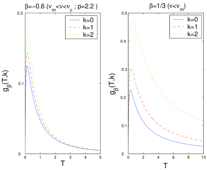
Figure 2: $g_{\beta}(\widetilde{T},k)$ for different $k$ values. Left) $\nu_{m}<\nu<\nu_{c}$; The differences between the shape of the pulses are small. The rise and the decay times are similar for different $k$ values, and the the peaks’ heights ratios between different $k$ pulses are less then 1.5. Right) $\nu<\nu_{m}$; The differences between the shape of the pulses are large, mainly in the decay time. Therefore, at this spectral segment it is important to consider the changes in $k$ when the density varies.

Spherically symmetric energy variations are most likely to occur due to refreshed shocks, when new inner shells arrive from the source and refresh the blast wave ( Rees & Meszaros 1998, Kumar & Piran 2000, Sari & Meszaros 2000). Kumar & Piran (2000) show that in such case the solution has a smooth transition from the BM solution with the energy of the pre-collision blast-wave ( the front shell) to another BM solution with the total energy of the two shells. The collision produces, however, a reverse shock whose emission has a lower peak frequency than the forward shock emission. Clearly our approximation fails to capture the effect of the reverse shock and it does not capture the details of the light curve during the time that the shock crosses the outer shell.

Our method enables a simple calculation of the observed light curve for a given density and energy profile. In Figures 3 and 4 we show the observed light curves for several different density profiles (with constant energy). Fig 3 depicts the $\nu_{m}<\nu<\nu_{c}$ light curve for a Gaussian ($\Delta R/R=0.1$) over-dense region in the ISM. Such a density profile may occur in a clumpy environment. The emission from a clump is similar to the emission from a spherically over-dense region as long as the clump’s angular size is much larger than $1/\gamma$. The different light curves are for a different maximal over-densities. We find that a maximal over-density of $5$ effects the observed light curve during two orders of magnitude in time. The effect of a maximal over-density of 40 is observed during four order of magnitude in time (note that in all the cases the width of the Gaussian is similar). Even a mild short length-scale, over-dense region (with a maximal over-density of 2) influences the light curve for a long duration (mainly due to the angular effects). This duration depends strongly on the magnitude of the over-density. Note that due to the nonlinear dependence of the observed flux on $n_{ext}$ a narrower Gaussian (smaller $\Delta R/R$) with an equivalent amount of mass in the over-dense region produces a larger fluctuation.

Fig 4 shows the observed light curve for several density jumps and drops. In the left panel $\nu_{m}<\nu<\nu_{c}$ at all times. In the right panel we compare the effect of similar density jumps on the light curve above and below $\nu_{c}$. When $\nu_{m}<\nu<\nu_{c}$ there is a transition from one power-law to another with the same power law index and a flux ratio factor of $(n_{2}/n_{1})^{1/2}$ between the two power-laws (as expected according to Sari et al. 1998). The duration of the transition is longer for larger density contrasts. This transition is observable for a duration of about two orders of magnitude in time for a density contrast of $10$ and for one order of magnitude in time for a density contrast of $2$. When $\nu_{c}<\nu$ (right panel) then after a small fluctuation, the light curve returns to behave as if there was no jump (or drop). The width of this fluctuation is between three orders of magnitude in time for high density contrast ($10$) to two orders of magnitude in time for small density contrast (2). The maximal amplitude obtained for a density jump is $\sim 20\%$ (a deviation of $\sim 0.2mag$) while the deviation for a density drop can reach $\sim 40\%$ (a deviation of $\sim 0.4mag$)

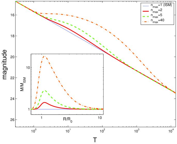
Figure 3: The light curves results from a Gaussian ($\Delta R/R=0.1$) over-dense region in the ISM. The different thick lines are for a maximal over-densities of $40$ (dashed-dot), $5$ (dashed) and $2$ (solid). The thin line is the light curve for a constant ISM density. The inset depicts the ratio of the mass, $M(R)$ over the mass of an ISM (without the over-dense region), $M_{ISM}(R)$.

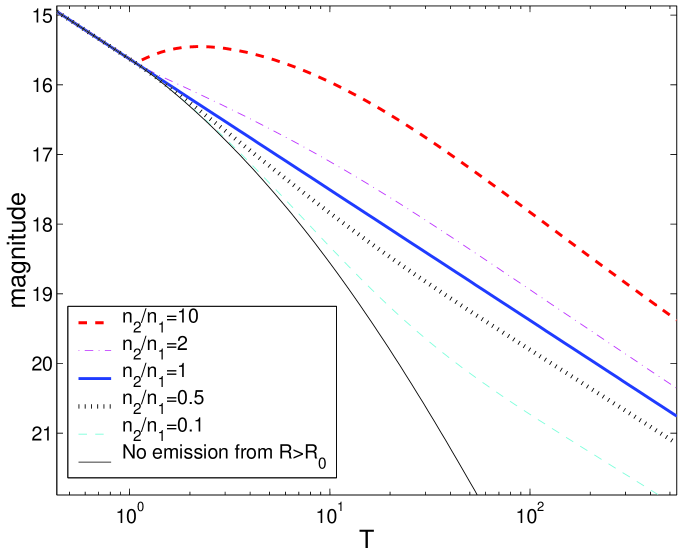
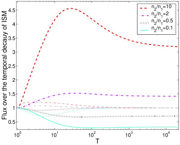
Figure 4: Left) The light curves for several density jumps and drops ($n=n_{1}$, $R<R_{0}$; $n=n_{2}$, $R>R_{0}$) for $\nu_{m}<\nu<\nu_{c}$. Right) The flux deviation from an ISM light curve produced by the same density jumps and drops for $\nu_{m}<\nu<\nu_{c}$ (bold lines) and $\nu_{c}<\nu$ (thin lines). In both panels the time, $T$, is normalized so $T_{los}(R_{0})=1$.

Now, using Eqs. 3-13 we can approximate the observed light curve for given energy and density profiles. However, for a given burst we usually have the observed light curve at hand and not the energy and density profiles at the source. In this case we can invert Eqs. 3-13 (numerically) under the assumption of either a constant energy or a constant density. Thus, we can find the profile of the free variable, which produces the observed light curve. The analytic approximation of $g_{\beta}$ (Eq. 17) greatly simplifies this inversion when $\nu_{m}<\nu$. The observed light curve at a given time is a convolution of emission at many different source times (or shock front’s radii). Inverting Eqs. 3-13 requires a de-convolution of the light curve to the emission at different radii. Unfortunately, deconvolution amplifies small errors in the observed data and the resulting de-convolved signal (or in our case the energy or density profile) is highly sensitive to small variations in the observed light curve.

In some cases the inversion of the observed light curve fails. This usually happens when the light curve depicts rapid decay. The angular and radial spreading dictates a fastest possible temporal decay (see Eqs. 6 and 17 in which $F_{\nu}\propto T^{-(2-\beta)}$ at late times). A faster temporal decay is impossible even if the emission from the blast wave completely stops. A faster observed temporal decay would result in a failure to invert Eqs. 3-13. This failure implies that a new effect (like angular dependence), which we do not consider, must be included.

4 GRB 021004

The peculiar afterglow of GRB 021004 was observed on October 4’th 2002. The early optical detection (Fox et al. 2002), $T\sim 500sec$, enabled a detailed observation of this afterglow from a very early stage. This unusual afterglow shows clear deviations from a smooth temporal power law decay. A first bump is observed at $T\sim 4000sec$, this bump is followed by a steep decay. Another smaller bump is observed at $T\sim 7\cdot 10^{4}sec$ and a possible third one at $3\cdot 10^{5}sec$. A steepening which may be a jet break is observed at $\sim 7days$. Several different mechanisms can lead to these observations. Some of the machisms suggested so far are external density variations, angular energy structure (patchy shell model), refreshed shocks, and a passage of $\nu_{m}$ through the optical band (Lazzati et al. 2002, Kobayashi & Zhang 2002, Nakar et al. 2002, Holland et al. 2002, Pandey et al. 2002, Bersier et al. 2002, Schaefer et al. 2002, Heyl & Perna 2002). The last scenario (the passage of $\nu_{m}$) explains only the first bump, and is combined with the emission of the reverse shock which should be dominant till the first bump.

In the following we apply our method to two possibilities (i): A spherically symmetric (or an angular scale larger then $1/\gamma$) density variations and constant energy; assuming that the optical emission is at all time above $\nu_{m}$ and below $\nu_{c}$, (ii) The passage of $\nu_{m}$ through the optical band, assuming an ISM density profile and a constant energy. Figure 5 depicts the best fit that we obtained with a spherically symmetric density variations with $p=2$. In order to get the fastest decay possible after the bump, we stop the emission completely at the peak of the bump. It is clear that due to the angular spreading, it is impossible to fit the fast decay after the first bump. The fit is even worse with larger $p$ . Figure 6 depicts the best fit of the first bump for a passage of $\nu_{m}$ through the R band in an ISM density profile and with a constant energy. Again, due to the angular spreading, it is impossible to fit the fast decay. We obtain a marginally consistent fast decay only if we assume that the emission is completely stopped just when $\nu_{m}$ is in the R-band. But clearly such a coincidence is unlikely.

The conclusion from these results is that it is unlikely that the light curve of GRB 021004 results from a spherically symmetric fluctuations. This result provides a new evidence that also in the early times of the GRB emission, an angular structure (either of the relativistic wind or the circum-burst medium) is involved.

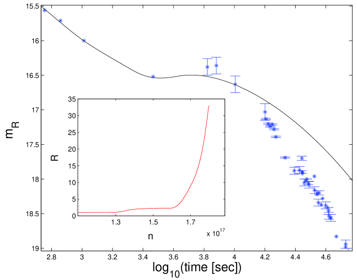
Figure 5: The best fit to the R-band observations of GRB 021004 (see the references to the GCNs at Nakar et al. 2002), using a varying density (and constant energy). We assume that $\nu_{m}<\nu<\nu_{c}$ at all times and we take $p=2$, $E=10^{52}\rm ergs$, $\varepsilon_{B}=0.01$ and $\varepsilon_{e}=0.1$. The inset depicts the density profile which produces this light curve. Note that at $R\sim 1.8\cdot 10^{17}$ The density drops to zero (the emission stops). Even though, the resulting light curve cannot fit the steep decay of the observations.

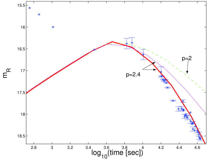
Figure 6: The best fit to the first bump in the R-band observations of GRB 021004 (see the references to the GCNs at Nakar et al. 2002), using the passage of $\nu_{m}$ through the optical band in an ISM density profile. The different thin lines are for $p=2$ (dashed) and $p=2.4$ (solid). The thick line is for $p=2.4$, assuming that the emission is completely stopped just when $\nu_{m}$ is in the $R$ band.

5 Conclusions

We have presented a simplified solution of the slow cooling synchrotron emission form a BM blast wave. This solution separates the observed flux at a given time to the contributions from different BM shells with a different radius of the shock front. Using the self-similar profile of the BM shells we have shown that the pulse shape of the emission from BM shells at different radii is general (independent of the shock’s front radius). We have also presented an analytic expression to this pulse shape for $\nu>\nu_{m}$. Thus, this pulse shape could be calculated only once (or the analytic expression may be used), and the whole solution turns into a simple one dimensional integral over the contributions from different radii. This simplification enables an easy calculation of different properties of the afterglow which until now had to be calculate using a complicate and computational time consuming simulations.

The main advantage of our solution is that it enables us to approximate the emission from a blast-wave with a varying energy and/or a varying external density, as long as these variations are spherically symmetric. The advantage of this solution over the method we have presented in Nakar et al. (2002) is the full consideration of the angular effects.

We use our solution to approximate the light curve which results from several density profiles. We find out that the duration of fluctuations in the light curve, which results from density variations, are long even if the length scale of the density variation, $\Delta R$, is very short ($\Delta R/R\ll 1$). For example a density variation with $\Delta R/R=0.1$ and a mild over-density results in a fluctuation which is observed for two orders of magnitudes in time. We show also that density variations induce mild ($\sim 30\%$) fluctuations also above $\nu_{c}$. Fluctuation induced by a density drop are larger than the fluctuation induced by a density jump. These fluctuations are also observed for about two orders of magnitude in time in the case of a sharp density jump, or drop.

We try to fit the early afterglow of GRB 021004, by a spherically symmetric varying density and by the passage of $\nu_{m}$ through the optical band. Both fits fail to follow the fast decay after the first bump in the afterglow. This results suggests that an angular structure within the ejecta or within the external density is crucial for the production of the early afterglow of GRB 021004.

Appendix: Derivation of the Light Curve Formula

In the appendix we show the details of the calculations which lead to Eqs. 3-14. First we solve the problem for $\nu<\nu_{c}$ and later we consider the solution for $\nu>\nu_{c}$.

We start from Eq. 2 which gives the observed flux from an arbitrary spherically symmetric emitting region. For $cos{\theta}=c(t-T)/r$ we obtain:

$$\Lambda(r,t)=\gamma(1-v\,\,cos\theta/c)\approx(2\gamma)^{-1}\left(1+\frac{T-T_{los}(r,t)}{T_{ang}(r,t)}\right).$$ (21)

At a given $t$, the front of the blast wave is at radius $R(t)$ and the emitting region is restricted to $r<R(t)$. On the other hand, emission from $r<r_{min}=c(t-T)=R(t)-c(T-T_{los}(R))$ would not reach the observer at time $T$. Hence, integrating over $cos{\theta}$ [$\delta(cos{\theta})=c\delta(t-T-rcos{\theta}/c)/r$], and keeping only terms of the lowest order of $\gamma^{-2}$, Eq. 2 is reduced to:

$$F_{\nu}(T)\approx\frac{2}{D^{2}}\int_{0}^{R_{max}}dR\int_{r_{min}}^{R}drr\gamma^{2}n^{\prime}(r)P^{\prime}_{\nu^{\prime}m}\left(\frac{\nu}{2\gamma\nu^{\prime}_{m}}\right)^{\beta}\left(1+\frac{T-T_{los}(r)}{T_{ang}(r)}\right)^{-(2-\beta)},$$ (22)

where $R_{max}$, is the maximal radius of the shock, from which an emission from the blast wave contributes to the flux at time $T$, i.e. $T_{los}(R_{max})=T$ . We also used the spectrum for $\nu<\nu_{c}$: $P^{\prime}_{\nu}(\nu\Lambda,r,t)=P^{\prime}_{\nu^{\prime},m}(r,t)\cdot(\nu\Lambda/\nu^{\prime}_{m})^{\beta}$, where $\nu^{\prime}_{m}$ is the synchrotron frequency in the fluid frame and $\beta$ is the spectral index.

The dependence of the hydrodynamical parameters in a BM self similar shell on $\chi$ is (BM76): the bulk Lorentz factor, $\gamma(\chi)=\Gamma\sqrt{1/2\chi}=\gamma(R)/\sqrt{\chi}$, the internal energy density in the fluid rest frame, $e^{\prime}(\chi)=e^{\prime}(R)\cdot\chi^{-(17-4k)/(12-3k)}$ and the fluid density behind the shock in the observer frame, $n(\chi)=n^{\prime}(\chi)\gamma(\chi)=n(R)\cdot\chi^{-(7-2k)/(4-k)}$, where $\gamma(R)$, $e(R)$ and $n(R)$ are the hydrodynamical parameters values at the shock front (at radius $R$). Now, We can express the observed synchrotron frequency, $\nu_{m}=2\gamma\nu^{\prime}_{m}(\chi)$, and the observed spectral power at this frequency $P_{\nu,m}=\gamma P^{\prime}_{\nu^{\prime},m}$ (Sari et al. 1998) as a function of $\chi$: $\nu_{m}(\chi)\propto\gamma B\gamma_{m}^{2}\propto\gamma(\chi)\sqrt{e(\chi)}\gamma_{m}^{2}(\chi)$ and $P_{\nu,m}(\chi)\propto\gamma(\chi)B\propto\gamma(\chi)\sqrt{e(\chi)}$, where $\gamma_{m}$ is the minimal Lorentz factor of the hot electrons distribution. In the slow cooling regime the radiative cooling of the electrons is negligible. The adiabatic cooling of a single electron is proportional to $e^{\prime}(\chi)/n^{\prime}(\chi)$, hence $\gamma_{m}(\chi)=\gamma_{m}(R)\cdot\chi^{-(2+2k)/(12-3k)}$. Now, we can represent all the variables in Eq. 22 as a function of the shock front, $R$, and the dimensionless parameter $\chi$ (which increase with the distance from the shock front). Integrating over $\chi$ [$dr=-d\chi R/2(4-k)\Gamma^{2}$] , using the relation:

$$\frac{T-T_{los}(r(\chi))}{T_{ang}(r(\chi))}=\frac{\widetilde{T}(R)}{\chi}-\frac{\chi-1}{2(4-k)\chi},$$ (23)

($\widetilde{T}(R)$ is defined in Eq. 7) and expressing the density behind the shock as $n(R)=2n_{ext}(R)\Gamma^{2}$ (see BM76) we obtain:

$$F_{\nu}(T)\approx\frac{2}{(4-k)D^{2}}\int_{0}^{R_{max}}A_{\nu}(R)g_{\beta}(\widetilde{T}(R),k)dR\quad\nu<\nu_{c},$$ (24)

where

$$A_{\nu}(R)=R^{2}n_{ext}(R)P_{\nu,m}(R)\left(\frac{\nu}{\nu_{m}(R)}\right)^{\beta}\quad\nu<\nu_{c}$$ (25)

and $g_{\beta}(\widetilde{T}(R),k)$ is defined by Eq. 6. Note that the emitted spectral power density depends on $\chi$ as: $\gamma^{2}n^{\prime}P^{\prime}_{\nu^{\prime}m}(\gamma\nu^{\prime}_{m})^{-\beta}\propto\chi^{-\mu(\beta,k)}$ ($\mu$ is defined in Eq. 8). The values of $\gamma(R)$, $\nu_{m}(R)$ and $P_{\nu,m}(R)$ could be found for any given external density profile (see Sari et al. 1998 and Nakar et al. 2002) as we have done in Eq. 5.

For $\nu>\nu_{c}$ the emitting electrons are cooling fast, and only a very thin layer behind the shock contributes to the emission at this spectral regime. Therefore the pulse shape of an instantaneous emission from a blast wave at radius $R$, $g_{\beta}(\widetilde{T},k)$, is similar to the pulse shape of an instantaneous emission from a very thin shell (see Eq. 1) with a spectral index of $\beta=-p/2$. Finelly, the emitted spectral power at the shock front, $A_{\nu}(R)$, is

$$A_{\nu}(R)=R^{2}n_{ext}P_{\nu,m}\nu_{m}^{-\beta}\nu^{1/2}_{c}\nu^{\beta-1/2}\quad\nu>\nu_{c},$$ (26)

where $\beta$ is the spectral index for $\nu_{m}<\nu<\nu_{c}$.

References

- (1) Bersier, D. et al., 2002, Submitted to ApJ (astro-ph/0211130)
- (2) Best, P. & Sari, R., 2000, Phys. Fluids. 12, 3029
- (3) Blandford, R. D., & Mckee, C. F., 1976, The physics of Fluids 19, 1130
- (4) Dai, Z. G. & Lu, T., 2002, ApJL, 565, L87
- (5) Fenimore, E., Madras, C. D. & Nayakshin, S., 1996, ApJ, 473, 998
- (6) Fox D.W., 2002, GCN 1564
- (7) Granot, J., Piran, T., & Sari, R., 1999 ApJ 513, 679
- (8) Granot, J. & Sari, R.,2002, ApJ, 568, 820
- (9) Heyl, J. & Perna, R., 2002 ApJL in press, (astro-ph/0211256)
- (10) Holland, S. et al., 2002, To appear in AJ (astro-ph/0211094)
- (11) Ioka, K. & Nakamura, T., 2001, ApJL, 554, L163
- (12) Kobayashi, S. & Zhang, B., 2002, ApJL, 582, L7
- (13) Kumar, P., & Piran, T., 2000a ApJ, 532, 286
- (14) Kumar, P.,& Piran, T., 2000b, ApJ, 535, 152
- (15) Kumar, P. & Panaitescu, A., 2000, ApJL, 541, L51
- (16) Lazzati, D., Rossi, E., Covino, S., Ghisellini, G., & Malesani D., 2002, AA, 396, L5
- (17) Nakar, E. , Piran, T, & Granot, J., 2002 accepted by NewA (astro-ph/0210631)
- (18) Pandey, S. B. et al. 2002, Submitted to BASI (astro-ph/0211108)
- (19) Perna, R. & Vietri, M.,2002, ApJL, 569, L47
- (20) Rees, M. J.& Meszaros, P., 1998, ApJL, 496, L1
- (21) Ryde, F. & Petrosian, V., 2002, ApJ, 578, 290
- (22) Sari, R., Piran, T., & Narayan, R., 1998, ApJL, 497, L17
- (23) Sari, R. & Meszaros, P., 2000, ApJL, 535, L33
- (24) Schaefer, B. et al., 2002, ApJ in press, (astro-ph/0211189)
- (25) Wang, X., Loeb, A. & Waxman, E. 2002, submitted to Phys. Rev. D (astro-ph/0212519)