The Large-Scale Extinction Map of the Galactic Bulge from the MACHO Project Photometry

Abstract

We present a $(V-R)$-based reddening map of about 43 square degrees of the Galactic bulge/bar. The map is constructed using template image photometry from the MACHO microlensing survey, contains 9717 resolution elements, and is based on $(V-R)$–color averages of the entire color-magnitude diagrams (CMDs) in 4 by 4 arc-minute tiles. The conversion from the observed color to the reddening follows from an assumption that CMDs of all bulge fields would look similar in the absence of extinction. Consequently, the difference in observed color between various fields originates from varying contribution of the disk extinction summed along different lines of sight. We check that our $(V-R)$ colors correlate very well with infrared and optical reddening maps. We show that a dusty disk obeying a ${\rm cosec}|b|$ extinction law, $E(V-R)=0.0274\,{\rm cosec}|b|$, provides a good approximation to the extinction toward the MACHO bulge/bar fields. The large-scale $(V-R)$-color and visual extinction map presented here is publicly available in the electronic edition of the Journal and on the World Wide Web.

Subject Headings: dust, extinction — Galaxy: center — Hertzsprung-Russel diagram — stars: statistics — surveys

1 Introduction

There is a great interest in the study of stars in the central Galactic region. Such investigations can answer questions about the structure and extent of the Galactic bar, the metallicity gradient in the inner Galaxy, the age of the dominant populations and their formation history. These features can, in turn, provide crucial boundary conditions for cosmological simulations that attempt to reproduce galaxies like the Milky Way at redshift $z=0$.

Most observations of the central Galaxy are still performed in the optical bands. Typical studies are carried out via two kinds of surveys: (1) rather shallow large-scale studies aimed at detecting spatial changes of stellar density, metallicity etc.; (2) deep investigations of small fields aimed at detailed analysis of the local stellar populations. Both treatments have to take into account extinction. In the first case, the removal of reddening is essential for reaching correct differential conclusions. In the second case, the fields selected for observations are preferentially placed in low-extinction windows (e.g., Baade’s Window), which allows detections of intrinsically fainter stars in observations with the same limiting magnitude. The selection of new target fields, therefore, benefits from large-scale maps of extinction.

There are a few extinction maps of the central Galactic region. The all-sky COBE/DIRBE map by Schlegel, Finkbeiner, & Davis (1998) covers this region, but there are suggestions that it overestimates the amount of dust in high-extinction areas (Stanek 1998; Arce & Goodman 1999; Dutra et al. 2003). Schultheis et al. (1999) used DENIS infrared data to construct a map of extinction in the Galactic plane with a latitude width of about three degrees. The MOA Project prepared an extinction map of 18 square degrees to determine the luminosity function for their analysis of microlensing events (Sumi et al. 2003). Dutra et al. (2003) investigated extinction of the central $10^{\circ}$ of the Milky Way by analyzing the available 2MASS data. These maps covered many degrees of the sky. Studies on smaller scales include Stanek’s (1996) map in Baade’s Window and the Frogel, Tiede, & Kuchinski (1999) map of several, small isolated fields, located mostly at two perpendicular lines: one at the Galactic longitude $l=0\mbox{$\hbox{$.\!\!^{\circ}$}$}0$, and another at the Galactic latitude $b=-1\mbox{$\hbox{$.\!\!^{\circ}$}$}3$.

Here, we use the optical $V$ and $R$ data (§2) from the MACHO experiment (e.g., Alcock et al. 1995) to construct a map of Galactic color with resolution of 4 arc-minutes. The method and the resultant map are discussed in §3 and 4, respectively. Our color map covers an area of about 43 square degrees and is based on all of the 94 MACHO bulge fields (http://wwwmacho.mcmaster.ca/Systems/Coords/Fields.html). This is a region that has not been fully covered by any other large-scale extinction map, except for Schlegel et al. (1998), which may not be reliable so close to the Galactic plane due to the presence of contaminating sources. In §5 we argue that the geometry of the dust distribution is well described by a very simple disk model. In §6 we show that for the fields located at the Galactic longitudes $l$ between 0 and 10 degrees and latitudes $b$ between $-2$ and $-10$ degrees our color map may be converted to an extinction map in a homogeneous fashion; three MACHO disk fields at $(l,b)\approx(18^{\circ},-2^{\circ})$ require a different treatment. This extinction map covers the Galactic latitude range that is sparsely probed by other compilations. We summarize our results in §7.

2 Data

We use the photometric data from the MACHO microlensing experiment. The MACHO experiment collected images of the Galactic bulge and Magellanic Clouds from 1992 through 1999. All observations were taken with the 1.3 m Great Melbourne Telescope with a dual-color wide-field camera. The MACHO camera consisted of two sets of four 2k x 2k CCDs that collected blue ($B_{M}$) and red ($R_{M}$) images simultaneously using a dichroic beam splitter. A single observed field covered an area of 43’ by 43’. Here we utilize a subset of the Galactic bulge observations from 94 MACHO fields.

As we are not interested in light curves of the stars, but rather in good representations of color-magnitude diagrams (CMD) of different sky regions, we base our photometry on template images. These are the images that were taken at the beginning of the MACHO experiment during particularly clear, good seeing nights. Overall, they provide the cleanest and most complete catalog of stars present in the MACHO data. Therefore, our CMDs are based on single-epoch photometry, but the fraction of stars with highly variable color is negligible and will not bias the mean colors we calculate. Each CMD is formed in a resolution element referred to as a “tile”. In MACHO terminology, tiles are specific and unique 4 by 4 arc-minute areas on the sky.

The great majority of the MACHO bulge photometry has not been calibrated and put on a uniform system. The only field that has a published calibration is MACHO field 119, which overlaps with Baade’s Window. To convert the MACHO instrumental magnitudes $B_{M}$ and $R_{M}$ to standard Johnson’s $V$ and Kron-Cousins $R$, we use the following relations:

$$V=23.70+0.82B_{M}+0.18R_{M}$$ (1)

and

$$R=23.41+0.18B_{M}+0.82R_{M}.$$ (2)

Calibrations (1) and (2) were obtained from equations (1) and (2) by Alcock et al. (1999), with $a_{0}$ and $b_{0}$ taken from their section 5.1, $a_{1}$ and $b_{1}$ taken from their Table 2, average airmass of about 1.04, and the bulge exposure time of 150s. We apply these $V$ and $R$ calibrations derived in field 119 to all our fields and do not make small-scale corrections for the focal plane spatial irregularities (e.g., chunk corrections). However, we apply global $(V-R)$ shifts to put all four CCD chips (0 to 3) on the same system, with chip # 1 serving as a reference. These global shifts are given in Table 1.

3 Our Method of Extinction Determination

Interstellar extinction is typically determined by comparing the measured color of an astronomical object (e.g., a star) with the known (calibrated) intrinsic color. The extinction can be estimated from two-band photometry using a group of tracers rather than individual stars. This statistical approach allows one to eliminate entirely erroneous measurements that may result from the wrong classification or anomalous character of an individual star. Stanek (1996) used the method of Woźniak & Stanek (1996) utilizing red clump giants to construct the map of extinction in Baade’s Window centered at Galactic $(l,b)=(1\mbox{$\hbox{$.\!\!^{\circ}$}$}0,-3\mbox{$\hbox{$.\!\!^{\circ}$}$}9)$. This map is based on the Optical Gravitational Lensing Experiment (OGLE) observations in $V$ and $I$ standard filters and covers about half a square degree on the sky. This map is intrinsically a map of relative extinction converting the local surface density of stars to the expected amount of dust. The currently accepted zero-point of extinction in this region was estimated by Gould, Popowski, & Terndrup (1998) and Alcock et al. (1998). Kiraga, Paczyński, & Stanek (1997) confirmed the reddenings derived by Stanek (1996) from clump giants using not only those stars but also two additional groups: subgiants and turnoff stars. By comparing the results from all three groups of tracers, Kiraga et al. (1997) showed that systematic errors of Stanek’s (1996) map are rather small.

There are two potential problems with Woźniak & Stanek’s (1996) approach. First, for a map with high resolution (like 30” by 30” one by Stanek 1996) there are generally few stars in a single resolution element and the result is affected by Poisson noise. Woźniak and Stanek (1996) partially solved this problem by ordering resolution elements according to the number of stars with $V<20.0$ mag and then binning this series. This procedure, however, introduces non-local correlations into a local estimate of extinction. This is part of a more general second problem, namely the fact that this procedure explicitly assumes that all the variations in stellar surface density are due to extinction. This may be approximately true in a small region like Baade’s Window, but will not be correct if one attempts to construct an extinction map of several square degrees.

Here, we propose a procedure that can circumvent the two above problems. First, it utilizes information stored in the whole set of observed stars and not in just a limited group. Second, it makes no assumptions about the underlying surface density of stars. The method is based on the single assumption that the intrinsic mean color of all observed stars (or their blends) in a given sky region is always the same. Of course, this assumption cannot be universally true. For example, we know that the CMD of the young disk population will be intrinsically noticeably bluer than the CMD of an old bulge population. Consequently, we would expect that the average of colors over all stars would be different. We argue in §6.1 that despite the considerable extent of the MACHO bulge region the first moment of the color distribution is dominated by the bar stars and only marginally affected by the changing contribution from the Galactic disk. Nevertheless, some uncontrolled sensitivity to a particular population mix in a given field remains the most serious systematic uncertainty of the method.

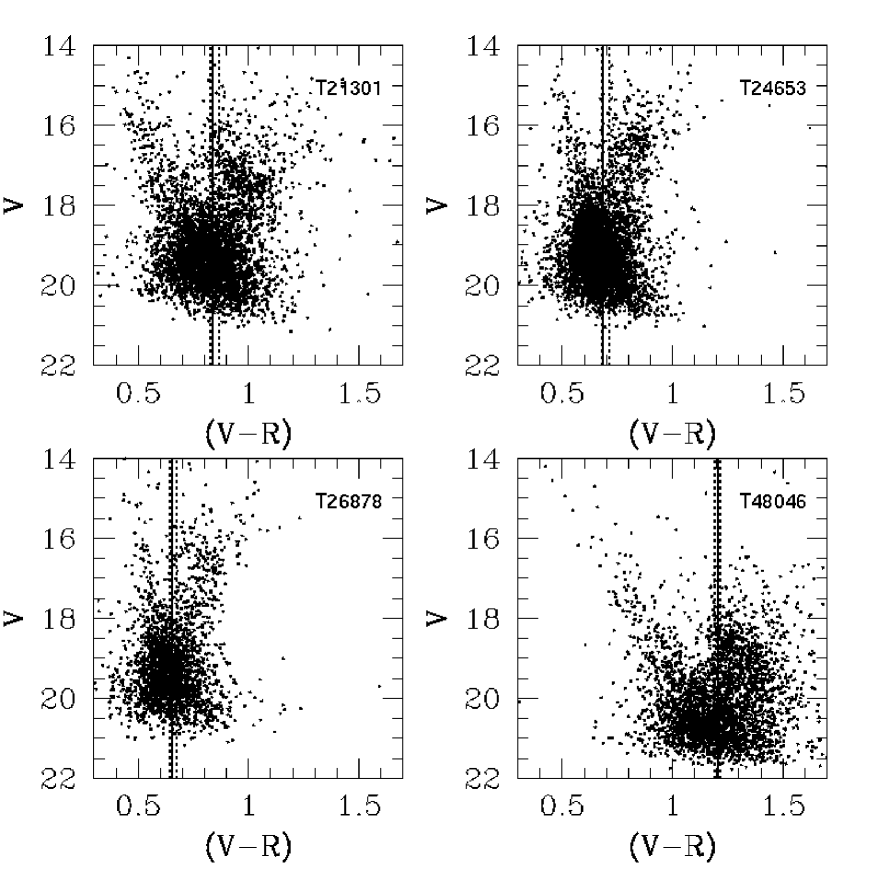
Figure 1: Four representative CMDs from the MACHO database. Tile names are given in the upper right corners. The solid line marks the average color. The dotted lines indicate the most extreme average colors obtained from analyzing partial CMDs containing stars either brighter of fainter than $V=19.0,20.0$. It is evident that the mean color is a very stable quantity with respect to simulated extinction bias.

For the MACHO experiment, the mean colors of CMDs are very weakly dependent on the limiting magnitude of the considered sample and, therefore, follow interstellar extinction and not morphology changes. This point is illustrated in Figure 1 which shows four representative CMDs selected from almost ten thousand analyzed in this work. The CMDs were selected to differ in morphology; the differences arise mostly from the various level of extinction. The numbers in the right upper corners are the MACHO tile labels. In each panel, the vertical solid line shows the average color of the entire CMD. We perform the following test. We divide each CMD into an upper and lower part at two values of $V$ magnitude: 19.0, and 20.0. Then we estimate the mean color of all four partial CMDs. The most extreme values are plotted with a dotted lines in each of the four considered CMDs. It is clear that a CMD color is very insensitive to the part of the diagram that we select, and thus the method presented here is robust with respect to the level of extinction. There are two reasons for this. First, if the faint parts of a CMD are removed (which mimics the effects of large extinction), the mean of color stays the same. Second, we find that the photometry in fields with large extinction typically reaches to fainter apparent magnitudes (compare, for example, T24653 and T48046). This is because the number of recovered stars is to a large extent crowding and not magnitude-limited. As a result, CMD morphology in fields with different extinction are more similar than one would naively expect.

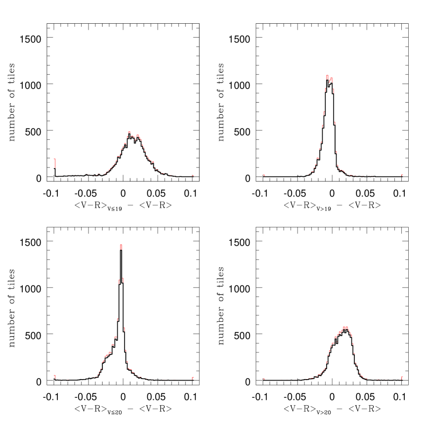
Figure 2: Histograms of the difference between average colors as computed from the entire MACHO CMD for a tile and the CMD cut at a certain $V$ magnitude, i.e., partial CMDs containing stars either brighter or fainter than $V=19.0,20.0$. In all cases, the difference is small and its distribution very narrow. The thin (red) line represents all 10466 non-empty tiles and the thick (black) line correspond to the tiles with more than 1000 stars.

The fact that the CMD magnitude cut has little effect on the mean of the color distribution is demonstrated in a statistical fashion in Figure 2, which is made for all non-empty bulge tiles at our disposal. The histograms presented in Figure 2 are centered close to 0.0 and are relatively narrow, which shows that our CMD-based method is robust in the considered range of extinctions.

4 The Map of Color

To avoid random fluctuations of the mean CMD color due to small number statistics and outliers, we eliminate all tiles with less than 1000 stars. This leaves us with 9717 tiles with well-defined mean colors. Most of the eliminated tiles are either entirely empty or only partially filled with stars. This is a result of the original MACHO procedure that divided the entire region in the sky into tiles, but then placed field centers without any reference to tiles’ positions. As the scatter in $(V-R)$ for stars in a CMD is almost always below 0.3 mags (and typically much smaller), allowing only CMDs with at least 1000 stars will result in a Poisson contribution of not more than 0.01 mag to the error in the average $(V-R)$. Therefore, the total error in an average color, $<V-R>$, will be dominated by the calibration errors.

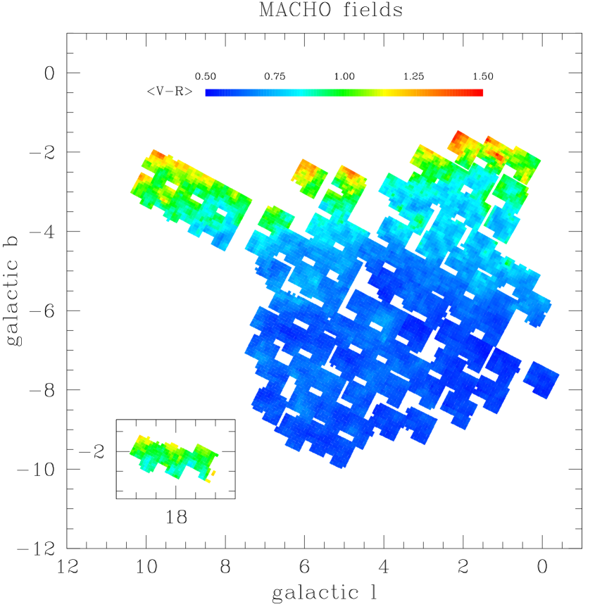
Figure 3: Color map of the central Galactic region. The scale is given at the top. Insert presents three disk fields separated from the others by $10^{\circ}$. The entire map is composed of 9717 resolution elements, 4’ by 4’ each.

The tiles that meet the above requirements are plotted in Figure 3. The color range is shown at the top. The fields in the insert are MACHO disk fields that are spatially separated from the others. We discuss them again in §6. When these three fields at $(l,b)\approx(18^{\circ},-2)^{\circ}$ are removed the sample consists of 9422 tiles.

Two facts are immediately obvious from Figure 3:

1. the variation in observed color is so large that differential extinction must be present since no population effects can produce such large differences (see §6),

2. on large scales, color (extinction) is regularly stratified parallel to the Galactic plane.

We will discuss these features and their consequences in the next sections.

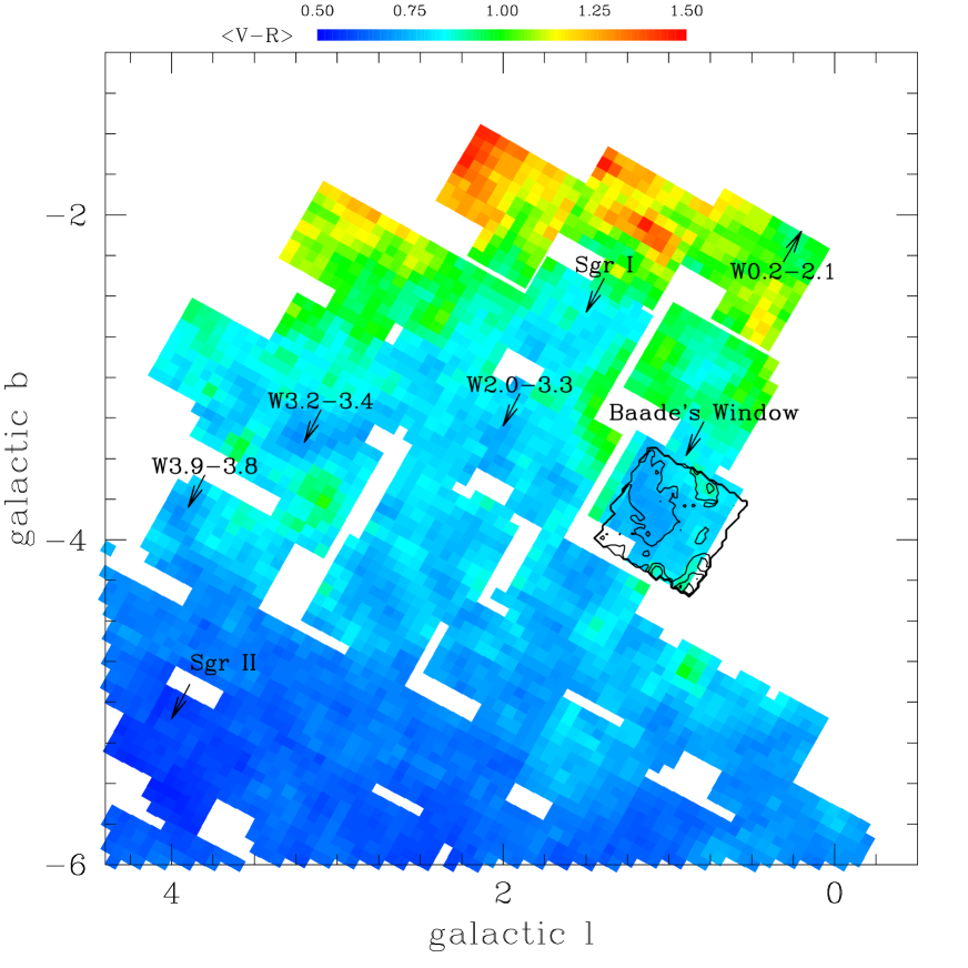
Figure 4: Color map showing details of the central Galactic region from Figure 3. The scale is given at the top. Stanek’s (1996) extinction contours are over-plotted on our Baade’s Window map. Additional low-extinction windows are marked with black arrows.

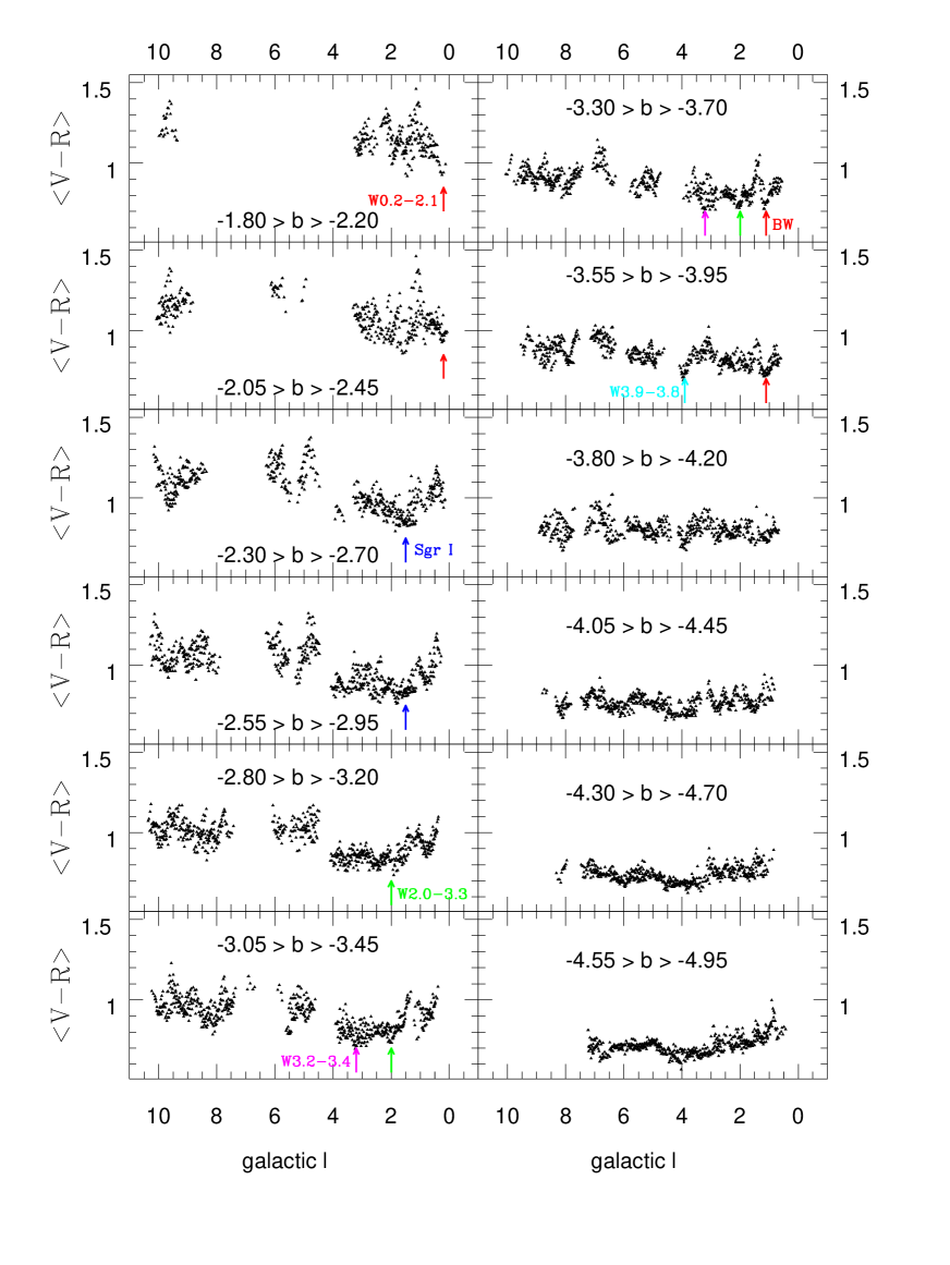
Figure 5: Color versus galactic longitude $l$ in strips covering a range of $0\mbox{$\hbox{$.\!\!^{\circ}$}$}4$ in galactic latitude $b$. Low extinction windows can be identified as troughs in color that persist for at least two strips. Only the first occurrence (from up to bottom and from left to right) is marked with a name – the remaining ones are indicated with arrows with identical color. A single possible low-extinction field at $(l,b)=(3\mbox{$\hbox{$.\!\!^{\circ}$}$}9,-3\mbox{$\hbox{$.\!\!^{\circ}$}$}8)$ is seen in only one $b$ strip, but the signal seems to be very strong.

Figure 4 is a detail of Figure 3 that concentrates on the fields closest to the Galactic center. Contours of constant extinction from Stanek (1996) are over-plotted on the Baade’s Window region. The agreement is excellent. We also mark several known and new low-extinction windows. These low-extinction areas are further investigated in Figure 5 where we present $<V-R>$ versus Galactic longitude $l$ in strips covering a range of $0\mbox{$\hbox{$.\!\!^{\circ}$}$}4$ in Galactic latitude $b$. Low-extinction windows can be identified as troughs in color that persist for at least two strips. A single possible low-extinction field at $(l,b)=(3\mbox{$\hbox{$.\!\!^{\circ}$}$}9,-3\mbox{$\hbox{$.\!\!^{\circ}$}$}8)$ is seen in only one $b$ strip, but the signal seems to be very strong. Using Figures 3, 4, and 5 we clearly identify all the currently known low-extinction windows in the MACHO $(l,b)$ quadrant (Baade 1963; Stanek 1998; Dutra, Santiago, & Bica 2002). They are listed in Table 2, where we also give the minimum $<V-R>$-color within $0.25^{\circ}$ of the approximate field center. Note that Sgr I window (Baade 1963) is not very pronounced in our maps. We also identify three entirely new low-extinction windows at $(l,b)$ of $(2\mbox{$\hbox{$.\!\!^{\circ}$}$}0,-3\mbox{$\hbox{$.\!\!^{\circ}$}$}3)$, $(3\mbox{$\hbox{$.\!\!^{\circ}$}$}2,-3\mbox{$\hbox{$.\!\!^{\circ}$}$}4)$, and $(3\mbox{$\hbox{$.\!\!^{\circ}$}$}9,-3\mbox{$\hbox{$.\!\!^{\circ}$}$}8)$. There is one possible low-extinction window somewhat farther away from the Galactic center at $(3\mbox{$\hbox{$.\!\!^{\circ}$}$}2,-6\mbox{$\hbox{$.\!\!^{\circ}$}$}4)$. However, the detection of this window is based on color that is uniformly bluer in one MACHO field. Thus it is not possible to conclude whether the effect is due to lower extinction or a particularly large calibration offset of this individual field.

5 The Dusty Disk

Observations of spiral galaxies (see NGC 891 for a beautiful example) suggest that dust is typically concentrated in a thin disk located in the plane of a galaxy. We will assume this geometry of the dust distribution for the Milky Way, and see whether it leads to a consistent picture. The simplest model of such a disk would be one with a fixed vertical structure that is axisymmetric and independent of the distance from the Galactic center. For a double exponential disk such a model would have an infinite scale length. If we make an additional assumption that all the stars we observe are behind the dust layer and that the Sun is located at the Galactic plane, then we will get a familiar cosec law:

$$E(V-R)=E_{\perp}(V-R)\,{\rm cosec}|b|,$$ (3)

where $E_{\perp}(V-R)$ is an average color excess in the direction perpendicular to the Galactic plane. In this model, the observed mean color is a sum of $E(V-R)$ and the intrinsic mean color of a CMD, $<V-R>_{0}$,

$$<V-R>=<V-R>_{0}+E_{\perp}(V-R)\,{\rm cosec}|b|.$$ (4)

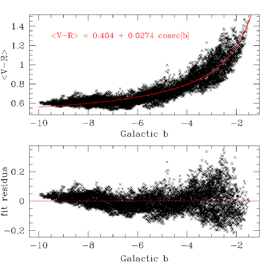
Figure 6: The red line displays the best fit of a simple cosec-law model of dusty disk. The upper panel present the fit, whereas the lower panel shows the residuals. The fit is based on 9422 resolution elements with the three disk fields at $(l,b)\approx(18^{\circ},-2^{\circ})$ excluded from the sample.

To avoid systematic effects associated with the analysis of different populations, we exclude the MACHO fields that are entirely dominated by the disk population: 301, 302, 303 at $(l,b)\approx(18^{\circ},-2^{\circ})$. However, we still retain fields 304–311 at $(l,b)\approx(8^{\circ},-2^{\circ})$. Therefore, we perform our computation based on measurements for 9422 tiles. The fit of equation (4) to the data is shown in the upper panel of Figure 6. The lower panel shows the residuals of this fit. The cone-like increase in the mean scatter with decreasing latitude is not necessarily a problem as this type of behavior is expected from more realistic disk models due to longitude dependence. Ignoring the scatter issue, there is a systematic trend in residuals suggesting that the model can be improved. Unfortunately, most of the exponential models of the Galactic disk share the problem apparent from Figure 6: it is very hard to achieve a very fast change in color at low Galactic latitudes and such a flat variation in the latitude range $(-6^{\circ},-10^{\circ})$. Nevertheless, the model (4) is a good zeroth order approximation to the data. We consider two sources of error: calibration errors in $<V-R>$ and Poisson errors in $<V-R>$ originating from the number of stars in a given CMD. We assume that the calibration error is identical in all cases. Therefore, the total error, ${\sigma}_{\rm tot}$, is given by

$${\sigma}^{2}_{\rm tot}={\sigma}^{2}_{<V-R>,{\rm cal}}+{\sigma}^{2}_{<V-R>,P}$$ (5)

We obtain the calibration error in $<V-R>$ by fixing the chi square of the fit to equal the number of degrees of freedom, $\chi^{2}/d.o.f=1$. Using this procedure, we obtain $\sigma_{<V-R>,{\rm cal}}\approx 0.064$. This value is consistent with the level of variation expected from the lack of a field-by-field calibration, but most likely is only an upper limit on the calibration error. The fact that model (4) is just a crude approximation to reality may be responsible for a large portion of $\sigma_{<V-R>,{\rm cal}}$. The best fit parameters for model (4) presented in the form with uncorrelated errors are:

$$<V-R>=(0.74156\pm 0.00066)+(0.02740\pm 0.00012)\,({\rm cosec}|b|-{\rm cosec}|-4\mbox{$\hbox{$.\!\!^{\circ}$}$}6513|).$$ (6)

The very small errors in equation (6) are internal errors. The systematic errors coming from uncertainty in the global zero points of photometry are much larger.

To obtain the results reported above we excluded three disk fields at $(l,b)\approx(18^{\circ},-2^{\circ})$. However, fit (4) may be extended to include two intrinsic colors, one for the bulk of the fields and the additional one just for fields 301, 302, and 303. The resultant $<V-R>_{0}$ for the high-$l$ fields is $0.15$ magnitudes bluer, which may be explained by our theoretical arguments from §6.1.

We would like to warn the reader against extensive use of eq. (6), since it provides a good representation only in the global sense. On the other hand, all the local features of reddening must be described by the detailed maps, like the one presented here.

6 Toward the Map of Extinction

6.1 General considerations

If we accept the conjecture that the color excess is associated with extinction, it is clear that we may bias the extinction measurement by an incorrect assumption about the intrinsic color. The fields that are dominated by the disk population should have bluer intrinsic color, and as a result higher extinction than the bulge-dominated fields with the same observed $<V-R>$. In addition, some foreground disk stars will not be affected by extinction, which would bias the observed mean color bluer and, as a result, artificially lower the inferred extinction. Here we estimate the biases caused by these effects.

Alcock et al. (2000) argue that in the MACHO bulge fields, the disk contribution to the number of stars down to $V=23$ is around 10%. Let us assume the same level of disk contribution for the MACHO stars considered here which were recovered with standard, point spread function photometry (with completeness dropping steeply at V = 21.5). Let us consider two types of CMDs: one entirely dominated by bulge stars with the intrinsic color $<V-R>_{0,B}$ and another one with $\xi_{d}=0.1$ disk contribution. If the intrinsic color of the pure disk population is $<V-R>_{0,D}\equiv<V-R>_{0,B}+\Delta_{DB}$ then the intrinsic color of the second type of CMD will be $<V-R>_{0,B}+\xi_{d}\,\Delta_{DB}$. We will take $\Delta_{DB}=-0.3$ indicating that the disk population is on average 0.3 mags bluer in $<V-R>$ than the bulge population. This is likely an upper limit as can be judged based on integrated colors of populations with different ages and metallicities (Girardi et al. 2002: the tables provided on their web page: http://pleiadi.pd.astro.it). This would suggest that a CMD entirely dominated by bulge stars has an intrinsic color that is only 0.03 mags redder than a CMD with a 10% disk contribution.

Now, let us estimate how the presence of foreground disk stars influences the inferred mean color and so biases the predicted extinction low. We want to estimate what fraction of the disk stars are affected by the total extinction and what fraction are less reddened. To obtain qualitative results we will assume that the scale height of the dusty disk is about 100 pc. In addition, we will make a simplifying assumption that all stars that are more than 100 pc from the plane experience full extinction and the ones that are less than 100 pc from the plane are foreground stars and experience no extinction. (These are very conservative assumptions with respect to estimating the effect of foreground stars on the CMD color since there are no stars that can avoid extinction entirely.) The fields closest to the Galactic plane (for the MACHO coverage, these are at $b\approx-2^{\circ}$) will be affected to the highest degree. For $b=-2^{\circ}$, the line of sight will be more than 100 pc from the plane in somewhat less than about 3 kpc, which is about a third of the distance toward the Galactic center. For a typical MACHO field location and a typical stellar disk model of the Milky Way, the number of disk stars observed in a given field is a weak function of the distance along the line of sight (e.g., Kiraga & Paczyński 1994). Therefore, in our simple model $f=1/3$ of the disk stars are in front and $(1-f)=2/3$ behind the extinction layer. Consequently, 1/3 of disk stars or 3% of all stars in such a CMD are extinction-free and the rest are reddened by the same amount independent of whether they belong to the disk or to the bar. Given $E_{\rm true}(V-R)$, we estimate the observed color excess of the mixed population to be equal to $E_{\rm obs}(V-R)=f\cdot\xi_{d}\cdot 0.0+((1-\xi_{d})+(1-f)\cdot\xi_{d})\cdot E_{\rm true}(V-R)=(1-f\cdot\xi_{d})\cdot E_{\rm true}(V-R)$. For a representative $E_{\rm true}(V-R)=0.5$, $E_{\rm obs}(V-R)=0.483$, so that the bias amounts to only $0.483-0.500=-0.017$ mags.

For the variation of the disk contribution expected in the MACHO bulge fields, both biases are negligible compared to the color excess itself. However, it can be seen from the above arguments that if the disk contribution is substantial, the difference in $(V-R)$-color excess between a given CMD and a pure bulge CMD can exceed 0.1 mags. We believe that this is exactly the reason why the disk fields presented in the insert in Figure 3 have systematically bluer color than their low-$l$ counterparts at similar $b$ values. Therefore, the fields dominated by the disk stars cannot be treated with the same extinction formulae as the bulk of the MACHO fields. That was also the motivation to exclude some of high longitude fields in the derivation of the dusty disk model in §5.

The MACHO bulge fields are situated in front of the tidal debris from the Sgr dwarf galaxy. The varying contribution of the Sgr Dsph at different locations could bias our results as well. This is not a serious concern at low Galactic latitudes as Sgr contribution to the number of stars, as traced by the RR Lyrae population, is on average less than 3% in these fields (Alcock et al. 1997). Therefore, the bias caused by variation in the number of Sgr stars should be substantially smaller than the contribution from the Galactic disk and so completely negligible. The situation is much harder to quantify in the MACHO fields that are farther away from the plane. Our investigation of RR Lyrae location and extinction (Kunder, Popowski, & Cook 2003, in preparation) will shed more light on this problem.

6.2 Extinction calibration through comparison with other reddening maps

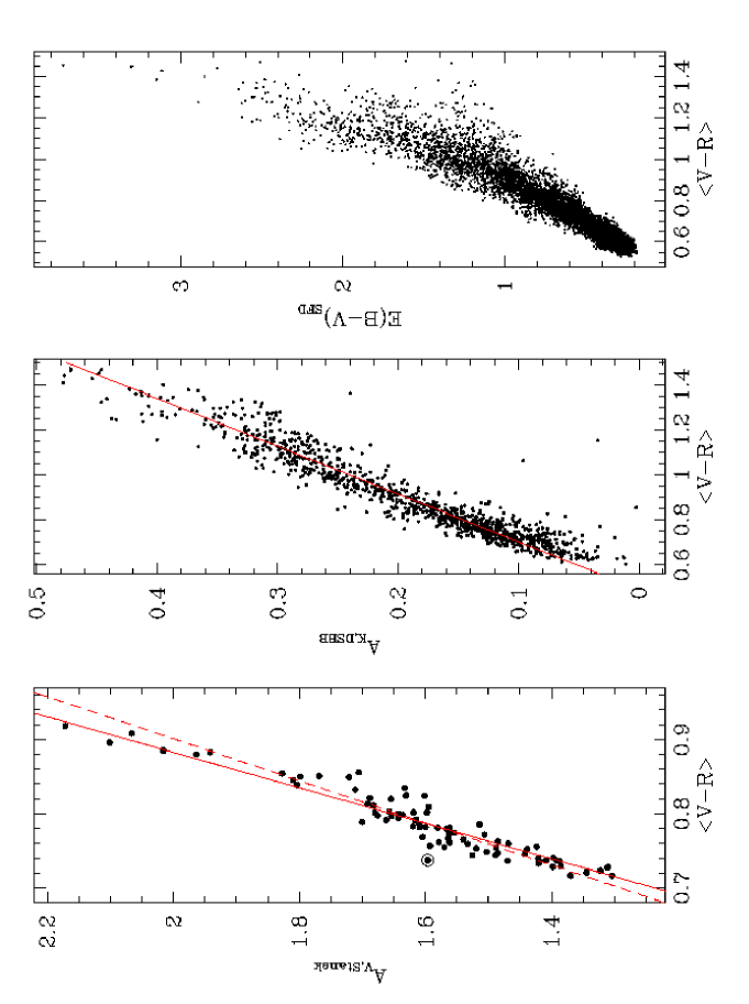
Figure 7: The left panel displays the relation between the mean color determined in this paper and extinctions obtained by Stanek (1996) for Baade’s Window. As the resolution of our map is lower than that of the OGLE-based extinction map in Baade’s Window, each $A_{V}$ value for comparison was obtained by averaging between 64 and 81 of Stanek’s (1996) 30” by 30” resolution elements. The dotted line represent equation (9) and the solid line equation (13). The excluded outlier is marked with a circled point. The middle panel presents the comparison with Dutra et al. (2003) values, that were based on the analysis of giant branches from 2MASS data. Here we plot their $A_{K}$ extinctions versus our $<V-R>$. We have matches for 1069 resolution elements. The span of $<V-R>$ is much wider than in the left panel. An over-plotted line comes from the scaled equation (11). In the right panel we plot Schlegel et al. (1998) reddenings based on COBE/DIRBE dust emission. Since the Schlegel et al. (1998) reddening map covers the entire sky, we matched all 9422 tiles from the bulge region. The relation between Schlegel et al. (1998) reddenings and $<V-R>$ is not linear. In summary, there is a strong correlation between an average color of the CMD $<V-R>$ and different reddening/extinction maps.

Figure 7 confirms that our interpretation of variation in mean color as due to differential extinction is correct. The left panel displays the relation between the mean color determined in this paper and extinctions obtained by Stanek (1996) for Baade’s Window. As the resolution of our map is lower than that of the OGLE-based extinction map in Baade’s Window, each $A_{V}$ value for comparison was obtained by averaging between 64 and 81 of Stanek’s (1996) 30” by 30” resolution elements. The 82 points in Figure 6 show a clear correlation between the visual extinction, $A_{V}$, and the mean stellar color, $<V-R>$. The middle panel presents the comparison with Dutra et al. (2003) values, that were based on the analysis of giant branches from 2MASS data. Here we plot their $A_{K}$ extinctions versus our $<V-R>$. We found the corresponding Dutra et al. (2003) values for about 1/9 of our resolution elements by selecting matched pairs on a one-to-one correspondence basis. This procedure resulted in 1069 matches, which span a much larger range in $<V-R>$ than the ones from Stanek (1996). Finally, in the right panel we plot Schlegel et al. (1998) reddenings obtained by feeding their software with the positions of our resolution elements. Since the Schlegel et al. (1998) reddening map covers the entire sky, we matched all 9422 tiles. The correlation between our color map and all the overlapping extinction maps is very strong. Therefore, our $(V-R)$-color map is an excellent map of relative reddening. For many practical applications one is interested in going one step further and inferring the value of extinction based on the observed color. We use Stanek (1996) and Dutra et al. (2003) data to derive the relations between the visual extinction $A_{V}$ and $<V-R>$. We do not make fits using Schlegel et al. (1998) map because $E(B-V)_{\rm SFR}$ versus $<V-R>$ relation cannot be universally fitted with a straight line. We discuss the calibrations based on maps by Stanek (1996) and Dutra et al. (2003) separately.

6.2.1 Extinction calibration based on Stanek’s (1996) map

We treat $<V-R>$ as an independent variable and fit a straight line of the following form:

$$A_{V}=a+b<V-R>.$$ (7)

The most straight forward interpretation of the fit parameters would imply that $b$ coincides with the coefficient of selective extinction and $a$ is a product of this coefficient and an intrinsic CMD color taken with a negative sign ($b\equiv R_{V,VR}$, $a\equiv-R_{V,VR}\,<V-R>_{0}$). We consider three sources of errors: calibration errors in $<V-R>$, Poisson errors in $<V-R>$ originating from the number of stars in a given CMD, and Poisson errors in $A_{V}$ coming from the scatter in Stanek’s (1996) extinctions. We assume that our calibration errors are identical in all cases. We assign all errors to the dependent variable.

Therefore, the total error, ${\sigma}_{\rm totBW}$, is given by

$${\sigma}^{2}_{\rm totBW}={\sigma}^{2}_{A_{V}}+b^{2}\left({\sigma}^{2}_{<V-R>,P}+{\sigma}^{2}_{<V-R>,{\rm calBW}}\right)$$ (8)

We obtain the calibration error of $<V-R>$ by fixing the chi square of the fit to equal the number of degrees of freedom, $\chi^{2}/d.o.f=1$. Application of this procedure to the data from Figure 6 results in ${\sigma}_{<V-R>,{\rm calBW}}=0.0157$, which dominates over the other sources of noise. If the calibration noise is Gaussian, then the expected number of points deviating from the fit by more than 2.75 sigma is $\approx 0.5$. Therefore, we will treat all points that deviate by more than 2.75 sigma as outliers, remove them, and repeat the fit. This procedure should make our results less prone to systematics. The one outlier is found at $2.98\sigma$. When removed, the $\chi^{2}$-normalized scatter drops to $\sigma_{<V-R>,{\rm calBW}}=0.0146$. We obtain the following fit presented in the form with uncorrelated errors :

$$A_{V}=(1.595\pm 0.006)+(3.52\pm 0.12)\left[<V-R>-0.7861\right]$$ (9)

Relation (9) is shown in Figure 7 as a dashed line. The circled point marks the excluded outlier.

There are three potential problems with solution (9):

1. all points with $<V-R>$ larger than 0.86 are above the fitted curve, which suggests some systematic trend;

2. the slope of $3.52\pm 0.12$ is much lower than the standard coefficient of selective extinction $R_{V,VR}\sim 5$ [The extinction toward the Galactic bulge may be anomalous as discussed by Popowski (2000) and Udalski (2003), but the value obtained here is rather extreme.];

3. zero extinction is reached only for $<V-R>_{0}=0.33\pm 0.02$, which is probably bluer than the colors of the bulge turn-off stars that determine the mean CMD color.

Note that equation (6) from §5 implies $<V-R>_{0}=0.4037\pm 0.0016$, which is $0.07$ magnitudes redder than $<V-R>_{0}=0.33\pm 0.02$ suggested by fit (9). This mismatch can originate from several sources. First of all, the zero point of Stanek’s (1996) extinction map can be overestimated by about $0.25$ mags. This is not very likely as this zero point has been accurately measured with two independent types of stars (Alcock et al. 1998; Gould et al. 1998).

Second, relation (4) is from the operational point of view indistinguishable from

$$<V-R>=<V-R>_{\rm const}+E_{\perp}(V-R)\,{\rm cosec}|b|,$$ (10)

where $<V-R>_{\rm const}$ can have two non-zero components: the intrinsic mean color of the CMD, $<V-R>_{0}$, and the uniform over-the-region component of extinction. In general, external information about the uniform extinction or intrinsic $<V-R>_{0}$ color of the bulge population would be needed to make a unique decomposition of $<V-R>_{\rm const}$. The color mismatch would be explained if a uniform extinction screen covered most of the MACHO Galactic fields with exception of Baade’s Window (and maybe few others). Two sources of possible uniform extinction: zodiacal dust and the Local Bubble are ineffective in producing significant extinction sheets. Schlegel et al. (1998) argue that the light to dust ratio for the material contributing to the zodiacal light is orders of magnitude larger than for ordinary interstellar matter. They estimate that zodiacal extinction is at the level of $10^{-6}$ mags in optical filters. The possible maximum contribution of the idealized bubble and the real geometry of the Local Bubble argue against a uniform layer of extinction of the required magnitude. Therefore, it is justified to assume that the constant term in equation (10) coincides with intrinsic color, that is $<V-R>_{\rm const}\approx<V-R>_{0}$.

This leaves us with the third option, namely, that some systematics in Baade’s Window chooses a $\chi^{2}$ minimum that is not a global minimum for all MACHO fields. This conclusion is supported by the very blue $<V-R>_{0}$ and anomalously small $R_{V,VR}$ reported in equation (9). When we fix $<V-R>_{0}=0.4037$, fit (7) to the Baade’s Window data from Figure 7 results in $R_{V,VR}=4.17\pm 0.01$ (solid line in the left panel). We believe that the above values are preferred over the ones returned by unconstrained fit (9), but the final resolution of the mismatch in intrinsic color will be addressed with a few thousand RR Lyrae stars (Kunder et al. 2003, in preparation) selected from the MACHO database.

6.2.2 Extinction calibration based on Dutra et al. (2003) map

We follow the route very similar to the one outlined in §6.2.1. To avoid any assumptions about the selective extinction coefficient, we try to recover the raw results from Dutra et al. (2003). Therefore, we convert their $A_{K}$ extinctions to $E(J-K_{s})_{\rm 2MASS}$ dividing all $A_{K}$ values by a factor of 0.670, which they used. For convenience, we then switch to $E(J-K)_{UKIRT}$ using color transformations given in http://www.ipac.caltech.edu/2mass/releases/allsky/doc/sec6_4b.html. We scale the errors in the same fashion. We derive the following fit presented in the form with uncorrelated errors:

$$E(J-K)_{\rm UKIRT}=(0.2430\pm 0.0024)+(0.657\pm 0.016)(<V-R>-0.839).$$ (11)

We detect no outliers. Appropriately scaled line (11) is shown in the middle panel of Figure 7. Result (11) is very insensitive to the level of the assumed MACHO field-to-field calibration errors, ${\sigma}_{<V-R>,{\rm cal}}$. The fit parameters change by less than 0.1% for ${\sigma}_{<V-R>,{\rm cal}}$ values between 0.02 and 0.064 mags, where the upper limit comes from the scatter derived during the analysis of the disk model in §5. To be specific, equation (11) was derived using ${\sigma}_{<V-R>,{\rm cal}}=0.02$ mag. We believe that the errors in the field-to-field calibration cannot be smaller than 0.02 mags. However even for this very low value, our fit results in $\chi^{2}/d.o.f.=0.167$. We conclude that Dutra et al. (2003) errors are too conservative. They are likely to be overestimated on average by at least a factor of 2.8.

For the one-parameter extinction curves from Cardelli, Clayton, & Mathis (1989) and O’Donnell (1994), the slope from equation (11) implies that $R_{V,VR}=4.56\pm 0.05$. Therefore, the visual extinction $A_{V}$ is given by:

$$A_{V}=-2.14+4.56\,<V-R>.$$ (12)

Equation (12) yields the intrinsic CMD color of $<V-R>_{0}=0.47$, substantially redder than what we derived from the Stanek (1996) map. Here, we do not attempt to fix the zero point to the value obtained from the dusty disk model, because our tiles matched to Dutra et al. (2003) resolution elements span wide enough range in $<V-R>$ to produce robust results.

Finally, we note that the total visual extinction out of the plane can be expressed as $A_{V,\perp}=R_{V,VR}\,E_{\perp}(V-R)$. Let us assume that $R_{V,VR}=4.4$, a representative value based on calibrations to Stanek (1996) and Dutra et al. (2003) extinctions. For $E_{\perp}(V-R)=0.0274$ taken from eq. (6), out-of-the-plane extinction $A_{V,\perp}=0.12$. It is interesting that this value obtained from observations close to the Galactic plane is consistent with results from extinction studies investigating the surroundings of the North Galactic Pole (e.g., Knude 1996).

7 Summary

We have constructed a $(V-R)$-color map of about 43 square degrees of the bulge/bar central region. This map has a resolution of 4’ by 4’ and is based on photometry from the MACHO microlensing survey. Each resolution element is assigned a color that is an average color of all stars detected in a tile from the MACHO template image. We selected only tiles with at least 1000 stars, and a typical tile contains a few thousand stars. We argued that average colors are insensitive to the details of the CMD morphology, which makes them a robust tool in the considered extinction range. We presented evidence that even a very simplistic cosec-law model of the Galactic dusty disk can qualitatively explain the observed distribution of mean color. However, we encourage the reader to use extinction maps whenever available, because the smooth disk model does not provide a good local approximation. We think that the geometry of the extinction layer revealed by the ${\rm cosec}\,|b|$ fit in Section 5 and observations of external galaxies argue strongly against the large amount of dust in the Galactic bulge itself. Even if an internal bulge extinction were present, the method implemented here would still work properly, because it simply measures the extinction toward the dominant population represented in a given CMD. However, the interpretation of the extinction as merely a mean value would become more important. At the moment, we interpret our reddenings as universally applicable to most stars observed toward the bulge lines of sight (except for a small number of foreground disk stars). Substantial internal reddening in the bulge would cause closer bulge stars to have overestimated reddenings and far ones to have underestimated reddenings. There would be no easy way to avoid this additional source of scatter.

Comparison with extinction maps by Stanek (1996), Schlegel et al. (1998), and Dutra et al. (2003) showed that the mean CMD colors correlate strongly with extinctions. Therefore, our color map can serve as an extinction map. Discussions in §5 and §6 suggest that there exists some uncertainty in fit parameters needed to convert CMD colors to visual extinctions. This question is being currently addressed through comparison of this color map with color excesses of RR Lyrae stars (Kunder et al. 2003, in preparation) selected from the MACHO database. For the time being, we give two possible prescription for obtaining $A_{V}$ from $<V-R>$:

$$A_{V}=-1.68+4.17\,<V-R>.$$ (13)

based on Stanek’s (1996) map and:

$$A_{V}=-2.14+4.56\,<V-R>.$$ (14)

based on the extinction determination by Dutra et al. (2003). The extinctions from the second calibration [eq. (14)] are about 0.2 mags lower for our weakly reddened fields with $<V-R>\sim 0.6$. The agreement is much better for $<V-R>\in(1.0,1.4)$. A complete extinction table will be published in the electronic version of the Journal. Table 3 provided here illustrates its format and content. The five columns list the positions in Galactic $(l,b)$ coordinates, $<V-R>$ - color, and two values of extinction calibrated according to equations (13) and (14). The uncertainty in extinction comes from two main sources: a mismatch between calibrations (13) and (14) discussed above and field-to-field calibration errors in $<V-R>$. When propagated to $A_{V}$, the field-to-field calibration errors are likely not smaller than $4.17\times 0.02$ and $4.56\times 0.02$ mags for the values derived from equations (13) and (14), respectively. We suggest using $\sigma_{A_{V}}=0.1$ mag as a lower limit in both cases. At the end of the electronic Table 3, we also include extinction estimates for the three disk fields at $(l,b)\approx(18^{\circ},-2^{\circ})$. We account for population effects in those fields by substituting $<V-R>$ with $(<V-R>+0.15)$ in equations (13) and (14). The color and extinction maps presented here are also available from http://www.mpa-garching.mpg.de/ popowski/bulgeColorMap.dat.

Table 1: CCD-related correction to $(V-R)$ colors

CCD designation	$(V-R)$ correction [mag]
chip 0	$-0.0639$string
chip 1	$0.0000$
chip 2	$-0.0072$string
chip 3	$-0.0377$string

Table 2: Low-extinction windows identified in the MACHO bulge data

Window name	Approximate location $(l,b)$	$<V-R>_{\rm min}$	Comment
Baade’s Window	$(1\mbox{$\hbox{$.\!\!^{\circ}$}$}1,-3\mbox{$\hbox{$.\!\!^{\circ}$}$}9)$	0.72	Baade (1963)
Sgr I	$(1\mbox{$\hbox{$.\!\!^{\circ}$}$}5,-2\mbox{$\hbox{$.\!\!^{\circ}$}$}6)$	0.81	Baade (1963)
Sgr II	$(4\mbox{$\hbox{$.\!\!^{\circ}$}$}0,-5\mbox{$\hbox{$.\!\!^{\circ}$}$}1)$	0.57	Baade (1963)
W0.2-2.1	$(0\mbox{$\hbox{$.\!\!^{\circ}$}$}2,-2\mbox{$\hbox{$.\!\!^{\circ}$}$}1)$	0.93	Stanek (1998), Dutra et al. (2002)
W2.0-3.3	$(2\mbox{$\hbox{$.\!\!^{\circ}$}$}0,-3\mbox{$\hbox{$.\!\!^{\circ}$}$}3)$	0.72	new
W3.2-3.4	$(3\mbox{$\hbox{$.\!\!^{\circ}$}$}2,-3\mbox{$\hbox{$.\!\!^{\circ}$}$}4)$	0.70	new
W3.9-3.8	$(3\mbox{$\hbox{$.\!\!^{\circ}$}$}9,-3\mbox{$\hbox{$.\!\!^{\circ}$}$}8)$	0.69	new
W3.2-6.4	$(3\mbox{$\hbox{$.\!\!^{\circ}$}$}2,-6\mbox{$\hbox{$.\!\!^{\circ}$}$}4)$	0.54	string new (?)

Table 3: Fragment of the extinction table

Galactic $l$	Galactic $b$	$<V-R>$	$A_{V}$ [mag]	$A_{V}$ [mag]
			calibrated to Stanek (1996)	calibrated to Dutra et al. (2003)
1.142	$-2.060$	1.462	4.42	4.53
1.143	$-3.852$	0.737	1.39	1.22
1.143	$-2.635$	0.858	1.90	1.77
1.144	$-4.679$	0.764	1.50	1.34
1.145	$-5.797$	0.625	0.93	0.71
1.148	$-5.944$	0.640	0.99	0.78
1.149	$-4.826$	0.789	1.61	1.46
1.149	$-3.999$	0.744	1.42	1.25
1.151	$-6.090$	0.592	0.79	0.56
1.151	$-2.208$	1.108	2.94	2.91
1.153	$-6.237$	0.576	0.72	0.49
1.154	$-4.973$	0.765	1.51	1.35
1.155	$-4.147$	0.785	1.60	1.44
1.155	$-3.466$	0.753	1.46	1.29
1.156	$-6.383$	0.593	0.79	0.57
1.157	$-1.821$	1.250	3.53	3.56

References

- (1) Alcock, C., et al. 1995, ApJ, 445, 133
- (2) Alcock, C., et al. 1997, ApJ, 474, 217
- (3) Alcock, C., et al. 1998, ApJ, 494, 396
- (4) Alcock, C., et al. 1999, PASP, 111, 1539
- (5) Alcock, C., et al. 2000, ApJ, 541, 734
- (6) Arce, H.C., & Goodman, A.A. 1999, ApJ, L135
- (7) Baade, W. 1963, Evolution of Stars and Galaxies, Harvard Univ. Press, Cambridge MA, p. 277
- (8) Cardelli, J.A., Clayton, G.C., & Mathis, J.S. 1989, ApJ, 345, 245
- (9) Dutra, C.M., Santiago, B.X., Bica, E. 2002, A&A, 381, 219
- (10) Dutra, C.M., Santiago, B.X., Bica, E.L.D., & Barbuy, B. 2003, MNRAS, 338, 253 (DSBB)
- (11) Frogel, J.A., Tiede, G.P., & Kuchinski, L.E. 1999, AJ, 117, 2296
- (12) Girardi, L., Bertelli, G., Bressan, A., Chiosi, C., Groenewegen, M. A. T., Marigo, P., Salasnich, B., Weiss, A. 2002, A&A, 391, 195
- (13) Gould, A., Popowski, P., & Terndrup, D.M. 1998, ApJ, 492, 778
- (14) Kiraga, M., & Paczyński, B. 1994, ApJ, 430, L101
- (15) Kiraga, M., Paczyński, B., & Stanek, K.Z. 1997, ApJ, 485, 611
- (16) Knude, J. 1996, A&A, 306, 108
- (17) O’Donnell, J.E. 1994, ApJ, 422, 158
- (18) Popowski, P. 2000, ApJ, 528, L9
- (19) Schlegel, D.J., Finkbeiner, D.P., & Davis, M. 1998, ApJ, 500, 525 (SFD)
- (20) Schultheis, M., et al. 1999, A&A, 349, 69
- (21) Stanek, K.Z. 1996, ApJ, 460, L37
- (22) Stanek, K.Z. 1998, preprint (astro-ph/9802307)
- (23) Sumi, T., et al. 2003, ApJ, 591, 204
- (24) Udalski, A. 2003, ApJ, 590, 284
- (25) Woźniak, P.R., & Stanek, K.Z. 1996, ApJ, 464, 233