A search for high redshift molecular absorption lines toward millimetre-loud, optically faint quasars

Abstract

We describe initial results of a search for redshifted molecular absorption toward four millimetre-loud, optically faint quasars. A wide frequency bandwidth of up to 23 GHz per quasar was scanned using the Swedish-ESO Sub-millimetre Telescope at La Silla. Using a search list of commonly detected molecules, we obtained nearly complete redshift coverage up to $z_{\rm abs}=5$. The sensitivity of our data is adequate to have revealed absorption systems with characteristics similar to those seen in the four known redshifted millimetre-band absorption systems, but none were found. Our frequency-scan technique nevertheless demonstrates the value of wide-band correlator instruments for searches such as these. We suggest that a somewhat larger sample of similar observations should lead to the discovery of new millimetre-band absorption systems.

1 Introduction

Millimetre-band (mm-band) molecular absorption systems along the line-of-sight to quasars provide a powerful probe of cold gas in the early Universe. Wiklind & Combes (1994a, 1995, 1996b) have used molecular absorption lines to study a variety of properties of the absorbers themselves (e.g. relative column densities, kinetic and excitation temperatures, filling factors etc.). Besides information about the absorbers, important cosmological parameters can be extracted from such data. Constraints on the cosmic microwave background temperature can be obtained by comparing the optical depths of different rotational transitions [e.g. CO(1–2), CO(2–3) etc.] (e.g. Wiklind & Combes, 1996c). Also, if the background quasar is gravitationally lensed, time delay studies can yield constraints on the Hubble constant (e.g. Wiklind & Combes, 2001). However, these studies have so far been limited by the paucity of mm-band molecular absorbers. Only 4 such systems are currently known: $z_{\rm abs}=0.685$ toward TXS 0218$+$357 (Wiklind & Combes, 1995), $z_{\rm abs}=0.247$ toward PKS 1413$+$135 (Wiklind & Combes, 1997), $z_{\rm abs}=0.672$ toward TXS 1504$+$377 (Wiklind & Combes, 1996a) and $z_{\rm abs}=0.886$ toward PKS 1830$-$211 (Wiklind & Combes, 1998).

Quasar absorption lines can also be used to search for possible variations in the fundamental constants. Detailed studies of the relative positions of heavy element optical transitions in 49 high redshift ($0.5<z_{\rm abs}<3.5$) absorption systems favour a smaller fine structure constant ($\alpha\equiv e^{2}/\hbar c$) at the 4.1 $\sigma$ significance level (Murphy et al., 2001c; Webb et al., 2001). The observed fractional change in $\alpha$ [$\Delta\alpha/\alpha=(-0.72\pm 0.18)\times 10^{-5}$] is very small and systematic errors have to be carefully considered. However, a thorough search for systematics has not revealed a simpler explanation of the optical results (Murphy et al., 2001a). Independent constraints at similar redshifts are required and recent attention has focused on molecular absorption systems.

Comparison of molecular rotational (i.e. mm-band) and corresponding H i 21-cm absorption line frequencies has the potential to constrain changes in $\alpha$ with a fractional precision $\sim\!10^{-6}$ per absorption system – an order of magnitude gain per absorption system over the purely optical methods. The ratio of the hyperfine (21-cm) transition frequency to that of a molecular rotational line is $\propto y\equiv\alpha^{2}g_{p}$ for $g_{p}$ the proton $g$-factor (Drinkwater et al., 1998). Thus, any variation in $y$ will be observed as a difference in the apparent redshifts, $\Delta y/y\approx\Delta z/(1+z)=(z_{\rm mol}-z_{\rm H})/(1+z_{\rm mol}$). Carilli et al. (2000) and Murphy et al. (2001b) have obtained constraints on $\Delta y/y$ consistent with zero $y$-variation from spectra of PKS 1413$+$135 and TXS 0218$+$357. Currently, the major uncertainty in this mm/H i comparison is that intrinsic velocity differences between the mm and H i absorption lines are introduced if the lines-of-sight to the mm and radio continuum emission regions of the quasar differ, as is certainly the case for PKS 1413$+$135 and TXS 0218$+$357 (Carilli et al., 2000).

Table 1: The source list. $S_{1.4}$, $S_{2.7}$,… $S_{230}$ are the measured 1.4, 2.7,… 230 GHz continuum flux densities in Jy. All values are obtained from the current version of the Parkes catalogue (Wright & Otrupcek, 1990), except ^aPhillips et al. (1995), the ^bNVSS catalogue (Condon et al., 1998), ^c (Teräsranta et al.1998), ^dKovalev et al. (1999) and ^eTornikoski, Lainela & Valtaoja (2000). No optical magnitudes are published for these objects. However, note that the sight-lines to both B 0648$-$165 and B 0727$-$115 suffer from moderate Galactic extinction, $A_{B}$ (Schlegel, Finkbeiner & Davis, 1998). Also, B 0500$+$019 is known to have an intervening H i absorption system. Since we do not reliably detect continuum emission from this quasar (see Fig. 1), we cannot place interesting limits on HCO⁺(1–2) or CO(2–3) absorption at 112.570 GHz and 218.227 GHz respectively.

Quasar	Coordinates (J2000)		$A_{B}$ (mag)	Radio flux densities (Jy)
	h  m  s	d   ′   ′′		$S_{1.4}$	$S_{2.7}$	$S_{5.0}$	$S_{8.4}$	$S_{11}$	$S_{22}$	$S_{86}$	$S_{230}$
B 0500$+$019/J 0503$+$203	05 03 21.2	02 03 05	0.289	2.10	2.46	2.04	1.61	1.36d	0.86d	–	–
B 0648$-$165/J 0650$-$1637	06 50 24.6	-16 37 40	2.456	1.70	1.40	1.02	0.80	–	–	0.9a	–
B 0727$-$115/J 0730$-$1141	07 30 19.1	-11 41 13	1.271	2.66b	1.95	2.22	3.36	3.87d	2.91d	0.9a	–
B 1213$-$172/J 1215$-$1731	12 15 46.8	-17 31 45	0.253	1.50	1.33	1.28	1.56	2.97d	2.44d	1.5a	$\approx 0.7^{c,e}$

A statistical sample of mm/Hi comparisons is therefore required to provide a reliable, independent check on the optical results for $\alpha$-variation. One systematic approach to finding more mm-band molecular absorbers is to scan the frequency space toward a sample of millimetre-loud quasars. Indeed, the absorber toward PKS 1830$-$211 was identified in this way by Wiklind & Combes (1996c). With the assumption that molecular absorption will be associated with significant optical extinction, one should select optically faint quasars to increase the probability of detecting molecular absorption. In this paper we present wide-band millimetre-wave spectra of the four millimetre-loud quasars which have not yet been optically identified: non-detections in the APM and DSS catalogues imply $m_{B}>20$. In the following section we describe the observations and data reduction and present the wide-band spectra. In Section 3 we search for possible millimetre absorption systems close to our detection limits. We make our conclusions and discuss the future of our search technique in Section 4.

2 Quasar spectra

2.1 Observations

We observed the quasars listed in Table 1 in February 2002 with the 15-m SEST at La Silla, Chile. The receivers were tuned to single-sideband mode and typical system temperatures, on the $T_{A}^{*}$-scale, were $\approx$250 K for the SESIS RX100 and RX150 receivers and $\approx$340 K and 480 K for the IRAM RX115 and RX230 respectively. The backends were acousto-optic spectrometers with 1440 channels and a channel width of 0.7 MHz. We used dual-beam switching with a throw of $\approx$12′ in azimuth, and pointing errors were typically $3\arcsec$ rms on each axis.

We used the SESIS and IRAM RX230 receivers for the majority of our integrations, providing the advantage of a wide (1 GHz) bandwidth (the IRAM RX115 has a 0.5 GHz bandwidth). Since the backend response decreases sharply toward the edges of the band, we overlapped the bands by observing at intervals of 0.8 GHz to ensure uniform signal-to-noise ratio (S/N) in the final, combined spectra. The lowest frequency we could tune the RX100 receiver to was 78.8 GHz and, although the nominal range is 78–116 GHz, the backend configuration did not allow tuning to 81.2, 82.0 or 82.8 GHz. Similarly, we could not tune the RX150 receiver to 141.7 or 142.5 GHz.

2.2 Data reduction

For each 1 GHz-wide spectrum, we averaged typically 10 two-minute (reference-subtracted) scans of the source and subtracted a low order polynomial fit from the data to provide a flat continuum. To convert the data from the $T_{A}^{*}$-scale to the Jy-scale we fitted a third-order polynomial to the aperture efficiency of SEST as a function of frequency:

$$S_{\nu}/{\rm Jy} = 7.55+0.340(\nu/{\rm GHz})-2.07\times 10^{-3}(\nu/{\rm GHz})^{2}$$ (1)

$$+5.32\times 10^{-6}(\nu/{\rm GHz})^{3}\,.$$

The intensity was calibrated using the chopper-wheel method which should be accurate to $\pm$10%. However, we found significant variations in the total flux density between each two-minute scan. Therefore, in Fig. 1 we present the mean flux density, $S_{\nu}$, for each of the 1 GHz-wide spectra with error bars representing the rms from the contributing scans.

Figure 1: The average flux densities, $S_{\nu}$, for each 1 GHz-wide portion of spectrum. The error bars represent the rms derived from typically 10 scans at each frequency, $\nu$. Power-law fits with the given parameters were used to define the continuum flux to which the spectra in Figs. 2–5 have been normalized.

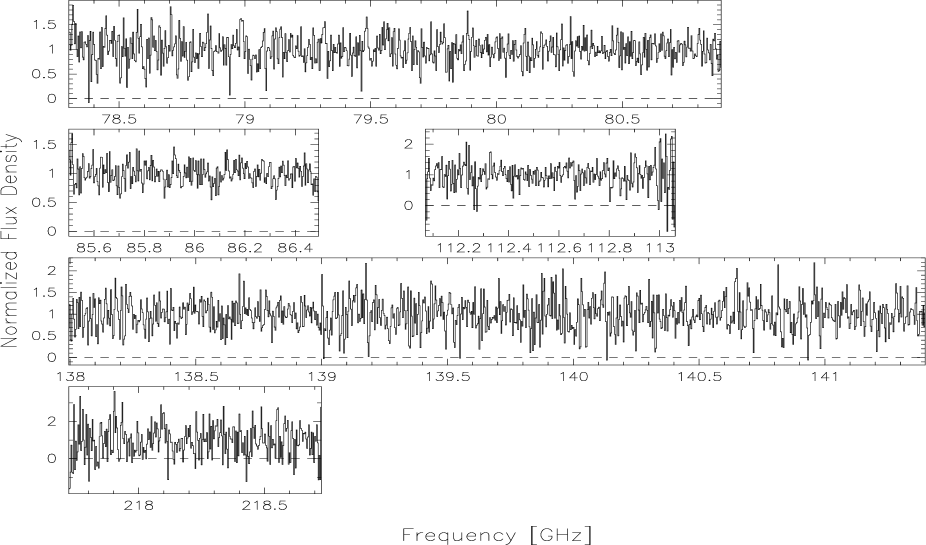
Figure 2: Wide-band spectrum of B 0500$+$019. These data (and those in Figs. 3–5) are normalized by the continuum flux of the quasar (taken as a power-law fit to the flux density data in Fig. 1) and, for clarity, have been boxcar-smoothed over 3 channels. The mean S/N = 1.72 per (unsmoothed) channel.

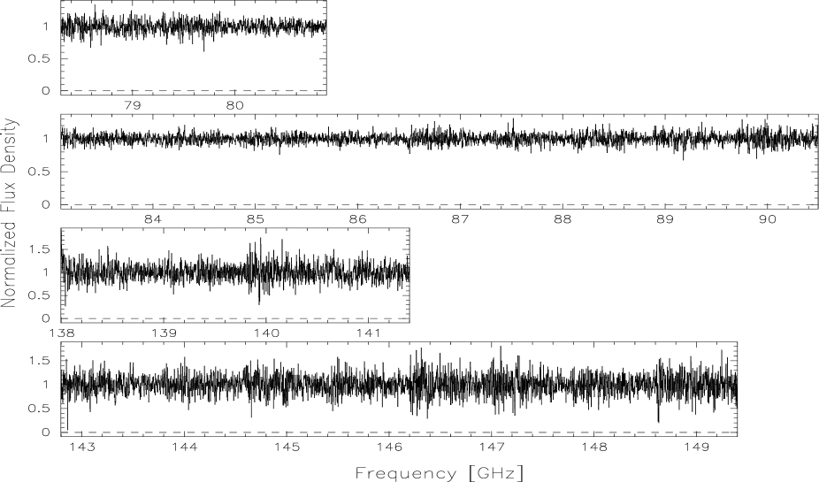
Figure 3: Wide-band spectrum of B 0648$-$165 (see caption to Fig. 2 for details). The mean S/N = 5.73 per (unsmoothed) channel.

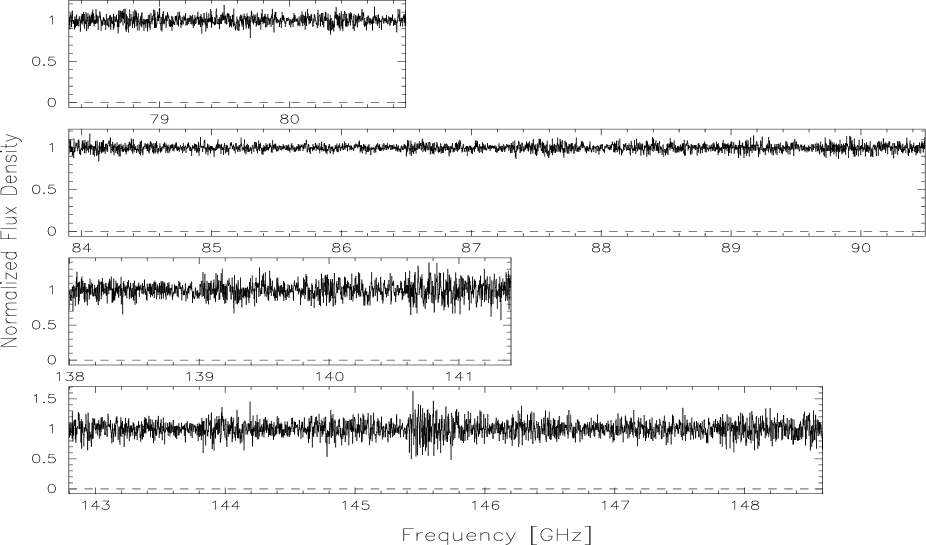
Figure 4: Wide-band spectrum of B 0727$-$115 (see caption to Fig. 2 for details). The mean S/N = 9.63 per (unsmoothed) channel.

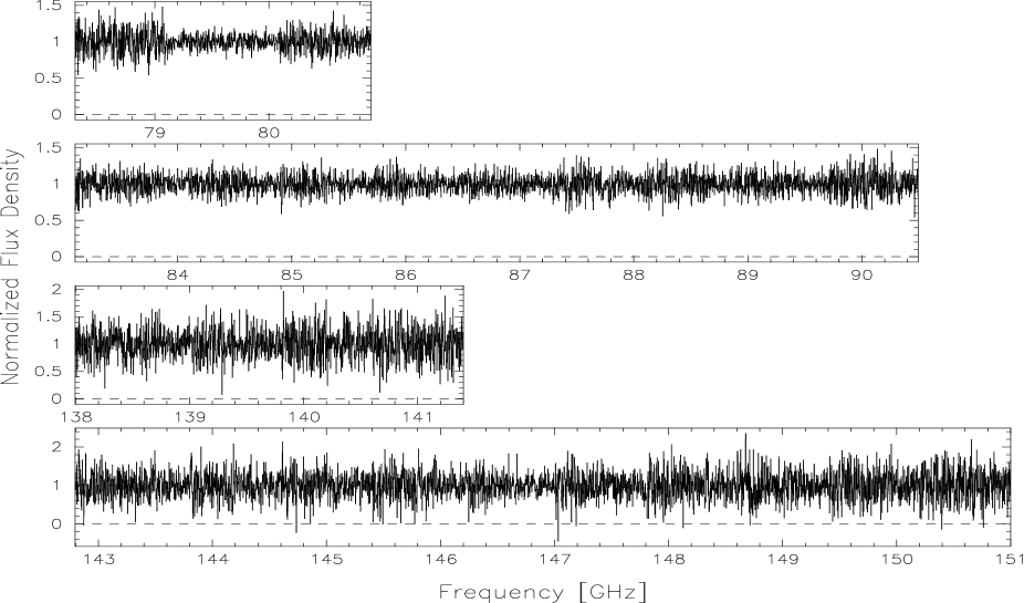
Figure 5: Wide-band spectrum of B 1213$-$172 (see caption to Fig. 2 for details). The mean S/N = 3.40 per (unsmoothed) channel.

For each channel, we generated a 1 $\sigma$ error from the rms in a window of width $2N_{\rm err}+1$ channels centred on that channel. We found that $N_{\rm err}=20$ provided reliable rms values but the results in Section 3.2 were insensitive to this parameter. In the 0.2 GHz regions where different 1 GHz-wide spectra overlapped, we re-sampled the variance-weighted average using the largest channel width of the contributing spectra. Finally, the combined spectra and 1 $\sigma$ error arrays were normalized to the flux density, $S_{\nu}$, of the quasars. $S_{\nu}$ was taken as a power-law fit to the flux densities presented in Fig. 1.

The combined spectra, normalized by the continuum, are presented in Figs. 2–5. Each contiguous spectral segment is plotted separately and all regions are plotted with the same linear frequency-scale. For clarity, the data have been boxcar-smoothed over 3 channels (we analyse the unsmoothed spectra in Section 3). From Fig. 2 it is clear that we only barely detect the continuum of B 0500$+$019. However, B 0648$-$165, B 0727$-$115 and B 1213$-$172 have S/N as high as $\approx$10 per (unsmoothed) 0.7 MHz channel. We obtained the largest spectral coverage on B 1213$-$172, a total (discontinuous) bandwidth of 23.2 GHz.

3 Searching for absorption systems

3.1 Search algorithm

Table 2 lists the transitions detected in the 4 known mm-band molecular absorption systems. From this table we selected a set of ‘commonly’ detected molecules for which to search in our observed spectra: CO, HCO⁺, HCN, HNC, CS and CN. We also searched for some common isotopomers of these molecules, which have lower terrestrial abundances, to provide potentially greater redshift space coverage and, as explained below, to help rule out some candidate absorption systems: ¹³CO, C¹⁸O, C¹⁷O, H¹³CO⁺, H¹³CN. For each molecule, we searched for all transitions lying below 1000 GHz (rest-frame) listed in the molecular line database of Pickett et al. (1998). With this fiducial set of transitions we obtain complete redshift coverage up to $z\approx 10$ for B 0648$-$165, B 0727$-$115 and B 1213$-$172. Since the frequency coverage for B 0500$+$019 is significantly smaller, several small redshift gaps (i.e. $\Delta z\la 0.05$) appear for $0.19<z<3.84$. However, the fraction of redshift space covered over this range is still high, $\approx$85%. The redshift coverage is complete for all other redshifts below $z\approx 10$.

Table 2: Transitions already detected in absorption at high redshift.

Transition	Quasara	Referenceb
CO(0–1)	B	WC94b
CO(1–2)	A,C	WC95; WC96a
CO(2–3)	A,C	WC95; WC96a
CO(3–4)	D	WC98
13CO(1–2)	A,C	WC95; WC96a
C18O(1–2)	A	CW95
HCO+(0–1)	B,D	WC97; CM02
HCO+(1–2)	A,B,C,D	WC95; WC96a,b,c
HCO+(2–3)	B,C,D	WC96a; WC96c; WC97
HCO+(3–4)	C	WC96a
H13CO+(0–1)	D	CM02
H13CO+(1–2)	D	WC98
HCN(1–2)	A,B,C,D	WC95; WC96a,b; WC97
HCN(2–3)	B,D	WC96c; WC97
HC3N(4–5)	D	CM02
H13CN(1–2)	D	WC98
HNC(0–1)	D	CM02
HNC(1–2)	B,C,D	WC96a,c; WC97
HNC(2–3)	B,C,D	WC96a,c; WC97
CS(0–1)	A	CWN97
CS(2–3)	D	WC96c
CS(3–4)	D	WC96c
N2H+(1–2)	D	WC96c
N2H+(2–3)	D	WC96c
H2CO($1_{10}$–$2_{11}$)	D	WC98
H2O(ortho)	A	CW98a
C3H2($1_{01}$–$2_{12}$)	D	CM02
LiH(0–1)	A	CW98b

^aQuasars: A = TXS 0218$+$357, B = PKS 1413$+$135, C = TXS 1504$+$377, D = PKS 1830$-$211. ^bReferences: CM02 (Carilli & Menten, 2002), CW95 (Combes & Wiklind, 1995), CWN97 (Combes, Wiklind & Nakai, 1997), CW98a (Combes & Wiklind, 1998a), CW98b (Combes & Wiklind, 1998b), WC94b (Wiklind & Combes, 1994b), WC95 (Wiklind & Combes, 1995), WC96a (Wiklind & Combes, 1996a), WC96b (Wiklind & Combes, 1996b), WC96c (Wiklind & Combes, 1996c), WC97 (Wiklind & Combes, 1997), WC98 (Wiklind & Combes, 1998).

In Fig. 6 we illustrate the redshift coverage up to $z_{\rm abs}=3.0$ achieved for B 1213$-$172 using only the strong (i.e. highest terrestrial abundance) isotopomers in the fiducial set. From the references in Table 2 it is clear that the transitions of HCN, HNC, CS and CN typically present a lower optical depth for absorption compared to CO and HCO⁺. Therefore, our estimate of the redshift range covered using the fiducial set of transitions may appear optimistic. The lower two panels in Fig. 6 compare the redshift coverage when using all the strong isotopomers with that obtained using only CO and HCO⁺. Though a noticeable decrease in the redshift coverage is clear, just using CO and HCO⁺ as a search diagnostic still allows much of the redshift space to be scanned. Note, however, that the third panel (from the bottom) in Fig. 6 shows that the redshifts covered by CO rarely overlap with those covered by HCO⁺. Thus, if one is to identify absorption systems with such a redshift scanning technique, one is biased toward finding systems containing strong HCN, HNC and perhaps CS and CN. This bias can only be avoided by observing wider-band spectra.

Figure 6: Schematic diagram illustrating the redshift coverage for B 1213$-$172 using only the strong (i.e. highest terrestrial abundance) isotopomers in the fiducial set. The upper six panels show the redshifts covered by each molecule given the frequencies observed (see Fig. 5). The vertical scale shows the lower-level rotational quantum number, $j$. The third panel from the bottom summarizes the coverage from all $j$-levels for each molecule. The panel marked ‘Total’ shows the coverage from all molecules and the lowest panel includes only the coverage from CO and HCO⁺. See text for discussion.

Using the 1 $\sigma$ error array for each spectrum, we slid a window of width $N_{\rm win}$ along the spectrum to search for absorption features above a significance level of $N_{\sigma}$ standard deviations. Note that the apparent significance of a candidate feature will be influenced by any correlations between the flux in adjacent channels. We address this problem in the simulations described in Section 3.2. Once an absorption feature is identified we associate it with a particular transition, allowing us to assign to it an absorption redshift, $z_{\rm abs}$, with an appropriate error, $\delta z_{\rm abs}$, which is taken as the redshift interval corresponding to the half-width of the feature. The ‘width’ is defined here as the number of channels over which the feature remains significant at a level $\geq N_{\sigma}$ standard deviations.

To identify an absorption system we search for another absorption feature which, when associated with a different transition, has a redshift $z_{\rm abs}\pm\delta z_{\rm abs}$. For computational convenience we impose an arbitrary but conservative redshift upper limit for absorption systems, $z_{\rm abs}\leq 5$. This upper limit can be extended to higher redshifts but our conclusions below are unchanged. Having identified a potential absorption system we can find the significance of absorption for all other transitions in the set defined above which fall within the bandpass of the spectrum.

Some of the candidate absorption systems can be immediately rejected using self-consistency conditions imposed by the relative ‘strengths’ of all available transitions. For example, if the detection of the absorption system relies on significant absorption in ¹³CO(1–2) but there is no significant absorption in CO(1–2) then we can rule out the putative detection. To form a rigid selection criteria, we found the integrated flux density, $S_{\rm int}$, and 1 $\sigma$ error, $\delta S_{\rm int}$, for the ‘host’ line [i.e. the weaker but higher terrestrial abundance line; CO(1–2) in the example above] and the significantly ‘detected’ line. In the analysis below we ruled out candidate systems if

$$S_{\rm int}^{\rm host}>S_{\rm int}^{\rm det}+2\,(\delta S_{\rm int}^{\rm host}+\delta S_{\rm int}^{\rm det})\,.$$ (2)

With the target transitions selected above, the fraction of absorption systems rejected in this way was typically $\sim$20%. Relaxing the criteria in equation 2 does not alter our main conclusions below.

3.2 Search results

Consistent with a visual inspection of Figs. 2–5, no strong (i.e. $\tau\sim 1$) absorption systems exist in our data. For all 4 quasars in our sample, no single-line absorption features were identified with $N_{\sigma}\geq 6.5\,\sigma$ for $3\leq N_{\rm win}\leq 31$. No absorption systems (i.e. double-line features) were observed for $N_{\sigma}\geq 5.4\,\sigma$. We list the strongest absorption system candidates in Table 3.

Table 3: The most significant double-line detections for each quasar in our sample. All transitions which fell into the band-pass of our observations are given and column 4 shows the significance of each detection (not corrected for correlations between data channels; negative values indicate flux values above the continuum). The final column gives the width in channels (as defined in Section 3.1), $\Delta$, of the two significant features responsible for the putative detection.

Quasar	$z_{\rm abs}$	Transitions	Sig. ($\sigma$)	$\Delta$
B 0500$+$019	2.81483	CS(10–11)	$4.5$	2
		CS(16–17)	$-1.0$
		C18O(2–3)	$4.8$	2
		HCO+(5–6)	$-2.1$
		HCN(5–6)	$0.6$
B 0648$-$165	2.02869	HCO+(4–5)	$4.3$	2
		HCO+(2–3)	$0.8$
		H13CO+(2–3)	$0.4$
		H13CO+(4–5)	$-0.8$
		13CO(3–4)	$0.9$
		C17O(3–4)	$0.0$
		C18O(3–4)	$1.9$
		HCN(2–3)	$5.4$	5
		HCN(4–5)	$0.0$
		HNC(2–3)	$0.3$
		CS(4–5)	$0.1$
		CS(8–9)	$0.9$
B 0727$-$115	1.51374	CN(1–2)	$4.2$	2
		13CO(1–2)	$0.1$
		C17O(1–2)	$3.0$
		C18O(1–2)	$4.9$	4
		H13CO+(3–4)	$0.4$
		HCN(3–4)	$-1.3$
		HNC(3–4)	$0.8$
B 1213$-$172	1.81705	C17O(1–2)	$4.4$	2
		CN(1–2)	$5.0$	4
		CS(4–5)	$2.1$
		CS(7–8)	$1.4$

Our search technique can be used to detect weaker absorption lines/systems by lowering the rejection limit, $N_{\sigma}$. However, this results in detection of large numbers of single and double-line features. For example, Fig. 7 shows the number of features detected in B 1213$-$172 if we set $N_{\sigma}=3.5\,\sigma$ (solid circles). To be sure that most of the these ‘weak candidates’ are spurious (i.e. the result of noise) we constructed synthetic spectra with the following procedure:

1. For each quasar, we modelled each 1 GHz integration as Gaussian noise with rms per channel equal to that of the real quasar data (i.e. the error arrays for the real and synthetic spectra were identical).

2. Each synthetic spectrum was convolved with a Gaussian with FWHM equal to that of the autocorrelation function of the quasar data.

3. We produced a final combined spectrum using the same procedure used for the real quasar spectra (see Section 2.2).

The effect of step (ii) is to introduce positive correlations between the flux density in neighbouring channels. We confirmed that the amplitude and range of correlations match those found in the real quasar data by comparing the autocorrelation functions for both data sets.

Figure 7: Number of single- and double-line matches found for B 1213$-$172 (solid circles) compared with the number found in simulated data (crosses) for a range of $N_{\rm win}$ and $N_{\sigma}=3.5\,\sigma$. The 1 $\sigma$ error bars are derived from the rms of 200 simulations and the crosses represent the mean value.

In Fig. 7 we compare the number of single- and double-line detections in our spectrum of B 1213$-$172 with a Monte Carlo simulation using synthetic spectra produced with the above procedure. We note that the number of lines identified in the real and synthetic spectra are the same within the standard deviation of the simulations. We verified that this is true for the entire range $3<N_{\rm win}<31$ (i.e. line widths $5{\rm\,km\,s}^{-1}<\Delta v<80{\rm\,km\,s}^{-1}$) and for all rejection limits $3.0\,\sigma<N_{\sigma}<5.5\,\sigma$, suggesting that our simple model of the SEST data is adequate. Thus, we conclude that we have not detected a large number of weak absorption systems in the quasar data, though we cannot rule out single [or small numbers ($\sim$5) of] weak systems.

4 Discussion

We have selected 4 millimetre-loud quasars which have not been detected optically ($m_{B}>20$), possibly because an intervening absorption system causes a large visual extinction. Such dusty systems could lead to detectable mm-band absorption and so we have performed wide-band millimetre-wave spectral scans to search for absorption at arbitrary, unknown redshifts. After defining a set of commonly detected molecules, we searched for absorption with nearly complete redshift coverage up to $z_{\rm abs}=5$. No candidate absorption systems (i.e. two independent features attributable to transitions with a common redshift) could be identified where both features had a significance $>5.4\,\sigma$.

Simulations indicate that systems identified with lower significance are consistent with noise. However, as a reminder that we cannot completely rule out these putative detections, we provide the best absorption system candidates in Table 3. These can be regarded as priority targets for follow-up observations. For our highest S/N spectrum, that of B 0727$-$115, the 3 $\sigma$ optical depth limit is $\approx$0.3  per (unsmoothed) channel. This is comparable to the optical depth limits reached in searches for various molecules in damped Lyman-$\alpha$ absorption systems (see Curran et al. 2002 and references therein) and compares well with the optical depths of many transitions in the 4 known high-$z$ mm-band molecular absorbers (see references in Table 2). Therefore, despite our null result, it is clear that wide-band correlator systems can be used to efficiently search for molecular absorption systems at unknown redshifts.

This paper has been typeset from a TeX/ LaTeX file prepared by the author.

References

- Carilli & Menten (2002) Carilli C. L., Menten K. M., 2002, in Rickman H., ed., Highlights of Astronomy Vol. 12, IAU 24: Cold Dust and Gas at High Redshift. Astron. Soc. Pac., San Francisco, CA, U.S.A
- Carilli et al. (2000) Carilli C. L. et al., 2000, Phys. Rev. Lett., 85, 5511
- Combes & Wiklind (1995) Combes F., Wiklind T., 1995, A&A, 303, L61
- Combes & Wiklind (1998a) Combes F., Wiklind T., 1998a, The Messenger, 91, 29
- Combes & Wiklind (1998b) Combes F., Wiklind T., 1998b, A&A, 334, L81
- Combes et al. (1997) Combes F., Wiklind T., Nakai N., 1997, A&A, 327, L17
- Condon et al. (1998) Condon J. J., Cotton W. D., Greisen E. W., Yin Q. F., Perley R. A., Taylor G. B., Broderick J. J., 1998, AJ, 115, 1693
- Curran et al. (2002) Curran S. J., Murphy M. T., Webb J. K., Rantakyrö F., Johansson L. E. B., Nikolić S., 2002, A&A, 394, 763
- Drinkwater et al. (1998) Drinkwater M. J., Webb J. K., Barrow J. D., Flambaum V. V., 1998, MNRAS, 295, 457
- Kovalev et al. (1999) Kovalev Y. Y., Nizhelsky N. A., Kovalev Y. A., Berlin A. B., Zhekanis G. V., Mingaliev M. G., Bogdantsov A. V., 1999, A&AS, 139, 545
- Murphy et al. (2001a) Murphy M. T., Webb J. K., Flambaum V. V., Churchill C. W., Prochaska J. X., 2001a, MNRAS, 327, 1223
- Murphy et al. (2001b) Murphy M. T., Webb J. K., Flambaum V. V., Drinkwater M. J., Combes F., Wiklind T., 2001b, MNRAS, 327, 1244
- Murphy et al. (2001c) Murphy M. T., Webb J. K., Flambaum V. V., Dzuba V. A., Churchill C. W., Prochaska J. X., Barrow J. D., Wolfe A. M., 2001c, MNRAS, 327, 1208
- Phillips et al. (1995) Phillips R. B., Doeleman S., Beasley A. J., Dhawan V., 1995, BAAS, 27, 1300
- Pickett et al. (1998) Pickett H. M., Poynter R. L., Cohen E. A., Delitsky M. L., Pearson J. C., Muller H. S. P., 1998, J. Quant. Spectrosc. Radiat. Transfer, 60, 883
- Schlegel et al. (1998) Schlegel D. J., Finkbeiner D. P., Davis M., 1998, ApJ, 500, 525
- (17) Teräsranta H. et al., 1998, A&AS, 132, 305
- Tornikoski et al. (2000) Tornikoski M., Lainela M., Valtaoja E., 2000, AJ, 120, 2278
- Webb et al. (2001) Webb J. K., Murphy M. T., Flambaum V. V., Dzuba V. A., Barrow J. D., Churchill C. W., Prochaska J. X., Wolfe A. M., 2001, Phys. Rev. Lett., 87, 091301
- Wiklind & Combes (1994a) Wiklind T., Combes F., 1994a, A&A, 288, L41
- Wiklind & Combes (1994b) Wiklind T., Combes F., 1994b, A&A, 286, L9
- Wiklind & Combes (1995) Wiklind T., Combes F., 1995, A&A, 299, 382
- Wiklind & Combes (1996a) Wiklind T., Combes F., 1996a, A&A, 315, 86
- Wiklind & Combes (1996b) Wiklind T., Combes F., 1996b, in Shaver P. A., ed., Science with Large Millimetre Arrays. Springer-Verlag, Berlin, Germany, p. 86
- Wiklind & Combes (1996c) Wiklind T., Combes F., 1996c, Nat, 379, 139
- Wiklind & Combes (1997) Wiklind T., Combes F., 1997, A&A, 328, 48
- Wiklind & Combes (1998) Wiklind T., Combes F., 1998, ApJ, 500, 129
- Wiklind & Combes (2001) Wiklind T., Combes F., 2001, in Brainerd T. G., Kochanek C. S., eds, Gravitational Lensing. Astron. Soc. Pac., San Francisco, CA, U.S.A, p. 155
- Wright & Otrupcek (1990) Wright A., Otrupcek R., 1990, Technical report, Parkes catalogue. Australia Telescope National Facility, NSW, Australia