Density Estimators in Particle Hydrodynamics

We present the results of a study confronting density maps reconstructed by the Delaunay Tessellation Field Estimator (DTFE) and by regular SPH kernel-based techniques. The density maps are constructed from the outcome of an SPH particle hydrodynamics simulation of a multiphase interstellar medium. The comparison between the two methods clearly demonstrates the superior performance of the DTFE with respect to conventional SPH methods, in particular at locations where SPH appears to fail. Filamentary and sheetlike structures form telling examples. The DTFE is a fully self-adaptive technique for reconstructing continuous density fields from discrete particle distributions, and is based upon the corresponding Delaunay tessellation. Its principal asset is its complete independence of arbitrary smoothing functions and parameters specifying the properties of these. As a result it manages to faithfully reproduce the anisotropies of the local particle distribution and through its adaptive and local nature proves to be optimally suited for uncovering the full structural richness in the density distribution. Through the improvement in local density estimates, calculations invoking the DTFE will yield a much better representation of physical processes which depend on density. This will be crucial in the case of feedback processes, which play a major role in galaxy and star formation issues. The presented results form an encouraging step towards the application and insertion of the DTFE in astrophysical hydrocodes. We describe an outline for the construction of a particle hydrodynamics code in which the DTFE replaces kernel-based methods. Further discussion addresses the issue and possibilities for a moving grid based hydrocode invoking the DTFE, and Delaunay tessellations, in an attempt to combine the virtues of the Eulerian and Lagrangian approaches.

1 Introduction

Smoothed Particle Hydrodynamics (SPH) has established itself as the workhorse for a variety of astrophysical fluid dynamical computations (Lucy Lc77 (1977), Ginghold & Monaghan GinMon77 (1977)). In a wide range of astrophysical environments this Lagrangian scheme offers substantial and often crucial advantages over Eulerian, usually grid-based, schemes. Astrophysical applications such as cosmic structure formation and galaxy formation, the dynamics of accretion disks and the formation of stars and planetary systems are testament to its versatility and succesful performance (for an enumeration of applications, and corresponding references, see e.g. the reviews by Monaghan Mon92 (1992) and Bertschinger Ber98 (1998)).

A crucial aspect of the SPH procedure concerns the proper estimation of the local density, i.e. the density at the location of the particles which are supposed to represent a fair – discrete – sampling of the underlying continuous density field. The basic feature of the SPH procedure for density estimation is based upon a convolution of the discrete particle distribution with a particular user-specified kernel function $W$. For a sample of $N$ particles, with masses $m_{j}$ and locations ${\bf r}_{j}$, the density $\rho$ at the location ${\bf r}_{i}$ of particle $i$ is given by

$$\rho({\bf r}_{i})\,=\,\sum_{j=1}^{N}\,m_{j}\,W({\bf r}_{i}-{\bf r}_{j},h_{i})\,,$$ (1)

in which the kernel resolution is determined through the smoothing scale $h_{i}$. Notice that generically the scale $h_{i}$ may be different for each individual particle, and thus may be set to adapt to the local particle density. Usually the functional dependence of the kernel $W$ is chosen to be spherically symmetric, so that it is a function of $|{\bf r}_{i}-{\bf r}_{j}|$ only.

The evolution of the physical system under consideration is fully determined by the movement of the discrete particles. Given a properly defined density estimation procedure, the equations of motion for the set of particles are specified through a suitable Lagrangian, if necessary including additional viscous forces (see e.g. Rasio Ras99 (1999)).

In practical implementations, however, the SPH procedure involves a considerable number of artefacts. These stem from the fact that SPH particles represent functional averages over a certain Lagrangian volume. This averaging procedure is further aggravated by the fact that it is based upon a rather arbitrary user-specified choice of both the adopted resolution scale(s) $h_{i}$ and the functional form of the kernel $W$. Such a description of a physical system in terms of user-defined fuzzy clouds of matter is known to lead to considerable complications in realistic astrophysical circumstances. Often, these environments involve fluid flows exhibiting complex spatial patterns and geometries. In particular in configurations characterized by strong gradients in physical characteristics – of which the density, pressure and temperature discontinuities in and around shock waves represent the most frequently encountered example – SPH has been hindered by its relative inefficiency in resolving these gradients.

Given the necessity for the user to specify the characteristics and parameter values of the density estimation procedure, the accuracy and adaptibility of the resulting SPH implementation hinges on the ability to resolve steep density contrasts and the capacity to adapt itself to the geometry and morphology of the local matter distribution. A considerable improvement with respect to the early SPH implementations, which were based on a uniform smoothing length $h$, involves the use of adaptive smoothing lengths $h_{i}$ (Hernquist & Katz HK89 (1989)), which provides the SPH calculations with a larger dynamic range and higher spatial resolution. The mass distribution in many (astro)physical systems and circumstances is often characterized by the presence of salient anisotropic patterns, usually identified as filamentary or planar features. To deal with such configurations, additional modifications in a few sophisticated implementations attempted to replace the conventional – and often unrealistic and restrictive – spherically symmetric kernels by ones whose configuration is more akin to the shape of the local mass distribution. The corresponding results do indeed represent a strong argument for the importance of using geometrically adaptive density estimates. A noteworthy example is the introduction of ellipsoidal kernels by Shapiro et al. (SM96 (1996)). Their shapes are stretched in accordance with the local flow. Yet, while evidently being conceptually superior, their practical implementation does constitute a major obstacle and has prevented widescale use. This may be ascribed largely to the rapidly increasing number of degrees of freedom needed to specify and maintain the kernel properties during a simulation.

Even despite their obvious benefits and improvements, these methods are all dependent upon the artificial parametrization of the local spatial density distribution in terms of the smoothing kernels. Moreover, the specification of the information on the density distribution in terms of extra non physical variables, necessary for the definition and evolution of the properties of the smoothing kernels, is often cumbersome to implement and may introduce subtle errors (Hernquist H93 (1993), see however Nelson & Papaloizou NP94 (1994) and Springel & Hernquist SH02 (2002)). In many astrophysical applications this may lead to systematic artefacts in the outcome for the related physical phenomena. Within a cosmological context, for example, the X-ray visibility of clusters of galaxies is sensitively dependent upon the value of the local density, setting the intensity of the emitted X-ray emission by the hot intergalactic gas. This will be even more critical in the presence of feedback processes, which for sure will be playing a role when addressing the amount of predicted star formation in simulation studies of galaxy formation.

Here, we seek to circumvent the complications induced by the kernel parametrization and introduce and propose an alternative to the use of kernels for the quantification of the density within the SPH formalism. This new method, based upon the Delaunay Tessellation Field Estimator (DTFE, Schaap & van de Weygaert SW00 (2000)), has been devised to mould and fully adapt itself to the configuration of the particle distribution. Unlike conventional SPH methods, it is able to deal self-consistently and naturally with anisotropies in the matter distribution, even when it concerns caustic-like transitions. In addition, it manages to succesfully treat density fields marked by structural features over a vast (dynamic) range of scales.

The DTFE produces density estimates on the basis of the particle distribution, which is supposed to form a discrete spatial sampling of the underlying continuous density field. As a linear multidimensional field interpolation algorithm it may be regarded as a first-order version of the natural neighbour algorithm for spatial interpolation (Sibson Sib81 (1981), also see e.g. Okabe et al. Oketal00 (2000)). In general, applications of the DTFE to spatial point distributions have demonstrated its success in dealing with the complications of anisotropic geometry and dynamic range (Schaap & van de Weygaert SW00 (2000)). The key ingredient of the DTFE procedure is that of the Delaunay triangulation, serving as the complete covering of a sample volume by mutually exclusive multidimensional linear interpolation intervals.

Delaunay tessellations (Delone 1934; see e.g. Okabe et al. 2000 for extensive review) form the natural framework in which to discuss the properties of discrete point sets, and thus also of discrete samplings of continuous fields. Their versatility and significance have been underlined by their widespread applications in such areas as computer graphics, geographical mapping and medical imaging. Also, they have already found widespread application in a variety of ‘conventional’grid-based fluid dynamical computation schemes. This may concern their use as a non-regular application-oriented grid covering of physicalsystems, which represents a prominent procedure in technological applications. More innovating has been their use in Lagrangian ‘moving-grid’ implementations (see Mavripilis Mv97 (1997) for a review, and Whitehurst Wh95 (1995) for a promising astrophysical application).

It seems therefore a good idea to explore the possibilities of applying the DTFE in the context of a numerical hydrodynamics code. Here, as a first step, we wish to obtain an idea of the performance of a hydro code involving the use of DTFE estimates with respect to an equivalent code involving regular SPH density estimates. The quality of the new DTFE method with respect to the conventional SPH estimates, and their advantages and disadvantages under various circumstances, are evaluated by a comparison between the density field which would be yielded by a DTFE processing of the resulting SPH particle distribution and that of the regular SPH procedure itself. In this study, we operate along these lines by a comparison of the resulting matter distributions in the situation of a representative stochastic multiphase density field. This allows us to make a comparison between both density estimates in a regime for which an improved method for density estimates would be of great value. We should point out a major drawback of our approach, in that we do not really treat the DTFE density estimate in a self-consistent fashion. Instead of being part of the dynamical equations themselves we only use it as an analysis tool of the produced particle distribution. Nevertheless, it will still show the value of the DTFE in particle gasdynamics and give an indication of what kind of differences may be expected when incorporating in a fully self-consistent manner the DTFE estimate in an hydrocode.

On the basis of our study, we will elaborate on the potential benefits of a hydrodynamics scheme based on the DTFE. Specifically, we outline how we would set out to develop a complete particle hydrodynamics code whose artificial kernel based nature is replaced by the more natural and self-adaptive approach of the DTFE. Such a DTFE based particle hydrodynamics code would form a promising step towards the development of a fully tessellation based quasi-Eulerian moving-grid hydrodynamical code. Such would yield a major and significant step towards defining a much needed alternative and complement to currently available simulation tools.

2 DTFE and SPH density estimates

The methods we use for SPH and DTFE density estimates have been extensively described elsewhere (Hernquist & Katz HK89 (1989), Schaap & van de Weygaert SW00 (2000)). Here, we will only summarize their main, and relevant, aspects.

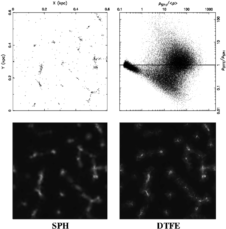
Figure 1: Comparison of the DTFE performance versus that of the regular SPH method in a characteristic configuration, that of a hydrodynamic simulation of the multiphase interstellar medium. Top left panel: the particle distribution in a $0.6\times 0.6$ kpc simulation region, within a slice with a width of 0.005 kpc. Bottom left frame: 2-D slice through the resulting (3-D) SPH density field reconstruction. Bottom right frame: the corresponding (3-D) density field reconstruction produced by the DTFE procedure. Top righthand frame: summary, in terms of a quantitative point-by-point comparison between the DTFE and SPH density estimates, $\rho_{\scriptstyle{\rm DTFE}}$ and $\rho_{\scriptstyle{\rm SPH}}$. Abscissa: the value of the SPH density estimate (normalized by the average density $\langle\rho\rangle$). Ordinate: the ratio of DTFE estimate to the SPH density estimate, $\rho_{\scriptstyle{\rm DTFE}}/\rho_{\scriptstyle{\rm SPH}}$. These quantities are plotted for each particle location in the full simulation box.

2.1 SPH density estimate

Amongst the various density recepies employed within available SPH codes, we use the Hernquist & Katz (HK89 (1989)) symmetrized form of Eq. 1, using adaptive smoothing lengths:

$${\hat{\rho}}_{i}\,=\,\frac{1}{2}\,\sum_{j}\,m_{j}\,\left\{W(|r_{i}-r_{j}|,h_{i})+W(|r_{i}-r_{j}|,h_{j})\right\}\,,$$ (2)

The smoothing lengths $h_{i}$ are chosen such that the sum involves around 40 nearest neighbours. For the kernel $W$ we take the conventional spline kernel described by Monaghan (Mon92 (1992)). Other variants of the SPH estimate produce comparable results.

2.2 DTFE density estimate

The DTFE density estimating procedure consists of three basic steps.

Starting from the sample of particle locations, the first step involves the computation of the corresponding Delaunay tessellation. Each Delaunay cell $T_{m}$ is the uniquely defined tetrahedron whose four vertices (in 3-D) are the set of 4 sample particles whose circumscribing sphere does not contain any of the other particles in the set. The Delaunay tessellation is the full covering of space by the complete set of these mutually disjunct tetrahedra. Delaunay tessellations are well known concepts in stochastic and computational geometry (Delaunay Del34 (1934), for further references see e.g. Okabe et al. Oketal00 (2000), Møller Mol94 (1994) and van de Weygaert Wey91 (1991)).

The second step involves estimating the density at the location of each of the particles in the sample. From the definition of the Delaunay tessellation, it may be evident that there is a close relationship between the volume of a Delaunay tetrahedron and the local density of the generating point process (telling examples of this may be seen in e.g. Schaap & van de Weygaert 2002a). Evidently, the “empty” cirumscribing spheres corresponding to the Delaunay tetrahedra, and the volumes of the resulting Delaunay tetrahedra, will be smaller as the number density of sample points increases, and vice versa. Following this observation, a proper density estimate ${\hat{\rho}}$ at the location ${\bf x}_{i}$ of a sampling point $i$ is obtained by determining the properly calibrated inverse of the volume ${\cal W}_{\scriptstyle{\rm Vor},i}$ of the corresponding contiguous Voronoi cell. The contiguous Voronoi cell ${\cal W}_{\scriptstyle{\rm Vor},i}$ is the union of all Delaunay tetrahedra $T_{m,i}$ of which the particle $i$ forms one of the four vertices, i.e. ${\cal W}_{\scriptstyle{\rm Vor},i}=\bigcup_{m}T_{m,i}$. In general, when a particle $i$ is surrounded by $N_{T}$ Delaunay tetrahedra, each with a volume ${\cal V}({T_{m,i}})$, the volume of the resulting contiguous Voronoi cell is

$${\cal W}_{\scriptstyle{\rm Vor},i}\,=\,\sum_{m=1}^{N_{T}}{\cal V}({T_{m,i}})\,.$$ (3)

Note that $N_{T}$ is not a constant, but in general may acquire a different value for each point in the sample. For a Poisson distribution of particles this is a non-integer number in the order of $\langle N_{T}\rangle\approx 27$ (van de Weygaert Wey94 (1994)). Generalizing to an arbitrary $D$-dimensional space, and assuming that each particle $i$ has been assigned a mass $m_{i}$, the estimated density ${\hat{\rho}}_{i}$ at the location of particle $i$ is given by (see Schaap & van de Weygaert SW00 (2000))

$${\hat{\rho}}({\bf r}_{i})\,=\,(D+1)\,\frac{m_{i}}{{\cal W}_{\scriptstyle{\rm Vor},i}}\,,$$ (4)

In this, we explicitly express ${\cal W}_{\scriptstyle{\rm Vor},i}$ for the general $D$-dimensional case. The factor $(D+1)$ is a normalization factor, accounting for the $(D+1)$ different contiguous Voronoi hypercells to which each Delaunay hyper“tetrahedron” is assigned, one for each vertex of a Delaunay hyper“tetrahedron”.

The third step is the interpolation of the estimated densities ${\hat{\rho}}_{i}$ over the full sample volume. In this, the DTFE bases itself upon the fact that each Delaunay tetrahedron may be considered the natural multidimensional equivalent of a linear interpolation interval (see e.g Bernardeau & van de Weygaert BerWey96 (1996)). Given the $(D+1)$ vertices of a Delaunay tetrahedron with corresponding density estimates ${\hat{\rho}}_{j}$, the value ${{\hat{\rho}}({\bf r})}$ at any location ${\bf r}$ within the tetrahedron can be straightforwardly determined by simple linear interpolation,

$${\hat{\rho}}({\bf r})\,=\,{\hat{\rho}}({\bf r}_{i0})\,+\,({\hat{\nabla\rho}})_{\scriptstyle{\rm Del},m}\,\cdot\,({\bf r}-{\bf r}_{i0})\,,$$ (5)

in which ${\bf r}_{i0}$ is the location of one of the Delaunay vertices $i$. This is a trivial evaluation once the value of the (linear) density gradient $({\hat{\nabla\rho}})_{\scriptstyle{\rm Del},m}$ has been estimated. For each Delaunay tetrahedron $T_{m}$ this is accomplished by solving the the system of $D$ linear equations corresponding to each of the remaining $D$ Delaunay vertices constituting the Delaunay tetrahedron $T_{m}$. The “minimum triangulation” property of Delaunay tessellations underlying this linear interpolation, minimum in the sense of representing a volume-covering network of optimally compact multidimensional “triangles”, has been a well-known property utilized in a variety of imaging and surface rendering applications such as geographical mapping and various computer imaging algorithms.

2.3 Comparison

Comparing the two methods, we see that in the case of SPH the particle ‘size’ and ‘shape’ (i.e. its domain of influence) is determined by some arbitrary kernel $W(r,h_{i})$ and a fortuitous choice of smoothing length $h_{i}$ (assuming, along with the major share of SPH procedures, a radially symmetric kernel). In the case of the DTFE method the particles’ influence region is fully determined by the sizes and shapes of the Delaunay cells $T_{m,i}$, themselves solely dependent on the particle distribution. In other words, in regular SPH the density is determined through the kernel function $W({\bf x})$, while in DTFE it is solely the particle distribution itself setting the estimated values of the density. Contrary to the generic situation for the kernel dependent methods, there are no extra variables left to be determined. One major additional advantage is that it is therefore not necessary to worry about the evolution of the kernel parameters.

Both methods do display some characteristic artefacts in their density reconstructions (see Fig. 1). To a large extent these may be traced back to the implicit assumptions involved in the interpolation procedures, a necessary consequence of the finite amount of information contained in a discrete representation of a continuous field. SPH density fields implicitly contain the imprint of the specified and applied kernel which, as has been discussed before, may seriously impart its resolving power and capacity to trace the true geometry of structures. The DTFE technique, on the other hand, does produce triangular artefacts. At instances conspicuously visible in the DTFE reconstructed density fields, they are the result of the linear interpolation scheme employed for the density estimation at the locations not coinciding with the particle positions. In principle, this may be substantially improved by the use of higher order interpolation schemes. Such higher-order schemes have indeed been developed, and the ones based upon the natural neighbour interpolation prescription of Sibson (Sib81 (1981)) have already been succesfully applied to two-dimensional problems in the field of geophysics (Sambridge et al. Sametal95 (1995), Braun & Sambridge BraSam95 (1995)) and solid state physics (Sukumar Suk98 (1998)).

     

Figure 2: Systematic analysis of the differences between the DTFE and SPH density estimates, $\rho_{\scriptstyle{\rm DTFE}}$ and $\rho_{\scriptstyle{\rm SPH}}$. Basis of the analysis is a point-by-point comparison of these two density estimates. Top lefthand frame: diagram of the value of the ratio $\rho_{\scriptstyle{\rm DTFE}}/\rho_{\scriptstyle{\rm SPH}}$ (ordinate) versus $\rho_{\scriptstyle{\rm SPH}}/\langle\rho\rangle$ (abscissa) for each of the points in the simulation volume. Indicated in this scatter diagram are four sectors, each of which corresponds to particles residing in a physically different regime/phase. On the basis of this identification, the full set of particles is dissected into the corresponding four composing particle samples. Top righthand frame: the spatial distribution of the full set of particles in a 0.04 kpc wide slice. The subsequent 4 frames (from central left to bottom right) show, for each indicated sector in the scatter diagram, the spatial distribution of the corresponding particles (within the same 0.04 kpc slice).

3 Case study: two-phase interstellar medium

For the sake of testing and comparing the SPH and DTFE methods, we assess a snapshot from a simulation of the neutral ISM. The model of the ISM is chosen as an illustration rather than as a realistic model.

The “simulation” sample of the ISM consists of HI gas confined in a periodic simulation box with a size $L=0.6\leavevmode\nobreak\$kpc³. The initially uniform density of the gas is $n_{H}=0.3$ cm^-3, while its temperature is taken to be $T=10000\leavevmode\nobreak\$K. No fluctuation spectrum is imposed to set the initial featureless spatial gas distribution. To set the corresponding initial spatial distribution of the $N=64000$ simulation particles, we start from relaxed initial conditions according to a “glass” distribution (e.g. White white94 (1994)).

The evolution of the gas is solely a consequence of fluid dynamical and thermodynamical processes. No self gravity is included. As for the thermodynamical state of the gas, cooling is implemented using a fit to the Dalgarno-McCray (DalCra72 (1972)) cooling curve. The heating of the gas is accomplished through photo-electric grain heating, attributed to a constant FUV background ($1.7$ G₀, with G₀ the Habing field) radiation field. The parameters are chosen such that after about 15 Myrs a two-phase medium forms which consists of warm ($10000$ K) and cold ($>100$ K) HI gas.

The stage at which a two-phase medium emerges forms a suitable point to investigate the performance of the SPH and DTFE methods. At this stage we took a snapshot from the simulation, and subjected it to further analysis. For a variety of reasons, the spatial gas distribution of the snapshot is expected to represent a challenging configuration. The multiphase character of the resulting particle configuration is likely to present a problem for regular SPH. Density contrasts of about four orders of magnitude separate dense clumps from the surrounding diffuse medium through which they are dispersed. Note that a failure to recover the correct density may have serious repercussions for the computed effects of cooling. In addition, we notice the presence of physical structures with conspicuous, aspherical geometries (see Fig. 1 & 2), such as anisotropic sheets and filaments as well as dense and compact clumps, which certainly do form a challenging aspect for the different methods.

3.1 Results

Fig. 1 offers a visual impression of the differences in performance between the SPH and DTFE density reconstructions. The greyscale density maps in Fig. 1 (lower left: SPH, lower right: DTFE) represent 2-D cuts through the corresponding 3-D density field reconstructions (note that contrary to the finite width of the corresponding particle slice, upper left frame, these constitute planes with zero thickness).

Immediately visible is the more crispy appearance of the DTFE density field, displaying substantially more contrast in conjunction with more pronounced structural features. Look e.g. at the compact clump in the lower righthand corner ($X\approx 0.5,Y\approx 0.12$), forming a prominent and tight spot in the DTFE density field. The clump at ($X\approx 0.48,Y\approx 0.52$) represents another telling example, visible as a striking peak in the DTFE rendering while hardly noticeable in the SPH reconstruction. Structures in the SPH field have a more extended appearance than their counterparts in the DTFE field, whose matter content has been smeared out more evenly, over a larger volume, yielding features with a significantly lower contrast. In this assessment it becomes clear that the DTFE reconstruction adheres considerably closer to the original particle distribution (top lefthand frame). Apparently the DTFE succeeds better in rendering the shapes, the coherence and the internal composition in the displayed particle distribution. At various locations, the DTFE even manages to capture structural details which seem to be absent in the SPH density field.

To quantify the visual impressions of Fig. 1, and to analyze the nature of the differences between the two methods, we plot the ratio $\rho_{\scriptstyle{\rm DTFE}}/\rho_{\scriptstyle{\rm SPH}}$ as a function of the SPH density estimate $\rho_{\scriptstyle{\rm SPH}}/\langle\rho\rangle$ (in units of the average density $\langle\rho\rangle$). Doing so for all particles in the sample (Fig. 1, top righthand, Fig. 2, top lefthand) immediately reveals interesting behaviour. The scatter diagram does show that the discrepancies between the two methods may be substantial, with density estimates at various instances differing by a factor of 5 or more.

Most interesting is the finding that we may distinguish clearly identifiable and distinct regimes in the scatter diagram of $\rho_{\scriptstyle{\rm DTFE}}/\rho_{\scriptstyle{\rm SPH}}$ versus $\rho_{\scriptstyle{\rm SPH}}/\langle\rho\rangle$. Four different sectors may be identified in the scatter diagram. Allowing for some arbitrariness in their definition, and indicating these regions by digits 1 to 4, we may organize the particles according to density-related criteria, roughly specified as (we refer to Fig. 2, top left frame, for the precise definitions of the domains):

1. low density regions:
   $\rho_{\scriptstyle{\rm SPH}}/\langle\rho\rangle\,<\,1$

2. medium density regions, DTFE smaller than SPH:
   $\rho_{\scriptstyle{\rm DTFE}}\,<\,\rho_{\scriptstyle{\rm SPH}}$;     $1<\rho_{\scriptstyle{\rm SPH}}/\langle\rho\rangle<10$

3. medium density regions, DTFE larger than SPH:
   $\rho_{\scriptstyle{\rm DTFE}}\,>\,\rho_{\scriptstyle{\rm SPH}}$;     $1<\rho_{\scriptstyle{\rm SPH}}/\langle\rho\rangle<10$

4. high density regions:
   $\rho_{\scriptstyle{\rm DTFE}}\,\gtrsim\,\rho_{\scriptstyle{\rm SPH}}$;      $\rho_{\scriptstyle{\rm SPH}}/\langle\rho\rangle\,>\,10$

The physical meaning of the distinct sectors in the scatter diagram becomes apparent when relating the various regimes with the spatial distribution of the corresponding particles. This may be appreciated from the five subsequent frames in Fig. 2, each depicting the related particle distribution in the same slice of width 0.04 kpc. The centre and bottom frames, numbered 1 to 4, show the spatial distribution of each group of particles, isolated from the complete distribution (top right frame, Fig. 2). These particle slices immediately reveal the close correspondence between any of the sectors in the scatter diagram and typical features in the spatial matter distribution of the two-phase interstellar medium. This systematic behaviour seems to point to truly fundamental differences in the workings of the SPH and DTFE methods, and would be hard to understand in terms of random errors. The separate spatial features in the gas distribution seem to react differently to the use of the DTFE method.

We argue that the major share of the disparity between the SPH and DTFE density estimates has to be attributed to SPH, mainly on the grounds of the known fact that SPH is poor in handling nontrivial configurations such as encountered in multiphase media. By separately assessing each regime, we may come to appreciate how these differences arise. In sector 1, involving the diffuse low density medium, the DTFE and SPH estimates are of comparable magnitude, be it that we do observe a systematic tendency. In the lowest density realms, whose relatively smooth density does not raise serious obstacles for either method, DTFE and SPH are indeed equal (with the exception of variations to be attributed to random noise). However, near the edges of the low density regions, SPH starts to overestimate the local density as the kernels do include particles within the surrounding high density structures. The geometric interpolation of the DTFE manages to avoid this systematic effect (see e.g. Schaap & van de Weygaert 2002a,b), which explains the systematic linear decrease of the ratio $\rho_{\scriptstyle{\rm DTFE}}/\rho_{\scriptstyle{\rm SPH}}$ with increasing $\rho_{\scriptstyle{\rm SPH}}/\langle\rho\rangle$. To the other extreme, the high density regions in sector 4 are identified with compact dense clumps as well as with their extensions into connecting filaments and walls. On average DTFE yields higher density estimates than SPH, frequently displaying superior spatial resolution (see also greyscale plot in Fig. 1). Note that the repercussions may be far-reaching in the context of a wide variety of astrophysical environments characterized by strongly density dependent physical phenomena and processes ! The intermediate regime of sectors 2 and 3 clearly connects to the filamentary structures in the gas distribution. Sector 2, in which the DTFE estimates are larger than those of SPH, appears to select out the inner parts of the filaments and walls. By contrast, the higher values for the SPH produced densities in sector 3 are related to the outer realms of these features. This characteristic distinction can be traced back to the failure of the SPH procedure to cope with highly anisotropic particle configurations. While it attempts to maintain a fixed number of neighbours within a spherical kernel, it smears out the density in a direction perpendicular to the filament. This produces lower estimates in the central parts, which are compensated for with higher estimates in the periphery. Evidently, the adaptive nature of DTFE does not appear to produce similar deficiencies.

4 The DTFE particle method

Having demonstrated the improvement in quality of the DTFE density estimates, this suggests a considerable potential for incorporating the DTFE in a self-consistent manner within a hydrodynamical code. Here, we first wish to indicate a possible route for accomplishing this in a particle hydrodynamics code through replacement of the kernel based density estimates (1) by the DTFE density estimates. We are currently in the process of implementing this. The formalism on which this implementation is based can be easily derived, involving nontrivial yet minor modifications. Essentially, it uses the same dynamic equations for gas particles as those in the regular SPH formalism, the fundamental adjustment being the insertion of the DTFE densities instead of the regular SPH ones. In addition, a further difference may be introduced through a change in treatment of viscous forces. Ultimately, this will work out into different equations of motion for the gas particles. A fundamental property of a DTFE based hydrocode, by construction, is that it conserves mass exactly and therefore obeys the continuity equation. This is not necessarily true for SPH implementations (Hernquist & Katz HK89 (1989)).

The start of the suggested DTFE particle method is formed by the discretized expression for the Lagrangian $L$ for a compressible, nondissipative flow,

$$L\,=\,\sum_{i}m_{i}\left(\frac{1}{2}v_{i}^{2}+u_{i}(\rho_{i},s_{i})\right)\,,$$ (6)

where $m_{i}$ is the mass of particle $i$, $v_{i}$ its velocity, $s_{i}$ the corresponding entropy and $u_{i}$ its specific internal energy. In this expression, $\rho_{i}$ is the density at location $i$, as yet unspecified. The resulting Euler-Lagrange equations are

$$\frac{dv_{i}}{dt}\,=\,-\sum_{j}m_{j}\left(\frac{\partial u_{j}}{\partial{\rho}_{j}}\right)_{\!\!s}\,\frac{\partial\rho_{j}}{\partial x_{i}}\,.$$ (7)

The standard SPH equations of motion then follow after inserting the SPH density estimate (Eq. 1). Instead, insertion of the DTFE density (Eq. 4) will lead to the corresponding equations of motion for the DTFE-based formalism. Note that the usual conservation properties related to Eq. 6 remain intact. After some algebraic manipulation, thereby using the basic thermodynamic relation for a gas with equation of state $P(\rho)$,

$$\left(\frac{\partial u_{i}}{\partial\rho_{i}}\right)_{\!\!s}\,=\,\frac{P_{i}}{\rho_{i}^{2}}\,,$$ (8)

we finally obtain the equations of motion for the gas particles (moving in $D$-dimensional space),

$$\frac{dv_{i}}{dt}\,=\,\frac{1}{D+1}\,\sum_{m=1}^{N_{T}}P({T_{m,i}})\,\frac{\partial{\cal V}(T_{m,i})}{\partial x_{i}}\,.$$ (9)

This expression involves a summation over all $N_{T}$ Delaunay tetrahedra $T_{m,i}$, with volumes ${\cal V}(T_{m,i})$, which have the particle $i$ as one of its four vertices. The pressure term $P({T_{m,i}})$ is the sum over the pressures $P_{j}$ at the four vertices $j$ of tetrahedron $T_{m,i}$, $P({T_{m,i}})=\sum P_{j}$.

As an interesting aside, we point out that unlike in the conventional SPH formalism, this procedure implies an exactly vanishing acceleration $dv_{i}/dt$ in the case of a constant pressure $P$ at each of the vertices of the Delaunay tetrahedra containing particle $i$ as one of their vertices. The reason for this is that one can then invoke the definition of the volume of the contiguous Voronoi cell corresponding to point $i$ (Eqn. 3), yielding

$$\frac{dv_{i}}{dt}\,=\,\frac{1}{D+1}\,P\,\frac{\partial{\cal W}_{Vor,i}}{\partial x_{i}}\,.$$ (10)

Since the volume of the contiguous Voronoi cell does not depend on the position of particle $i$ itself (it lies in the interior of the contiguous Voronoi cell), the resulting acceleration vanishes. Another interesting notion, which was pointed out by Icke (ick2002 (2002)), is that Delaunay tessellations also provide a unique opportunity to include a natural treatment of the viscous stresses in the physical system. We intend to elaborate on this possibility in subsequent work dealing with the practical implementation along the lines sketched above.

5 Delaunay tessellations
    and ‘moving grid’ hydrocodes

Ultimately, the ideal hydrodynamical code would combine the advantages of the Eulerian as well as of the Lagrangian approach. In their simplest formulation, Eulerian algorithms cover the volume of study with a fixed grid and compute the fluid transfer through the faces of the (fixed) grid cell volumes to follow the evolution of the system. Lagrangian formulations, on the other hand, compute the system by following the ever changing volume and shape of a particular individual element of gas (interestingly, the ‘Lagrangian’ formulation is also due to Euler eul1862 (1862), who employed this formalism in a letter to Lagrange, who later proposed these ideas in a publication by himself, lag1762 (1762); see Whitehurst Wh95 (1995)).

For a substantial part the success of the DTFE may be ascribed to the use of Delaunay tessellations as an optimally covering grid. This suggests that they may also be ideal for the use in moving grid implementations for hydrodynamical calculations. As in our SPH application, such hydrocodes with Delaunay tessellations at their core would warrant a close connection to the underlying matter distribution. Indeed, attempts towards such implementations have already been introduced in the context of a few specific, mainly two-dimensional, applications (Whitehurst Wh95 (1995), Braun & Sambridge BraSam95 (1995), Sukumar Suk98 (1998)). Alternative attempts towards the development of moving grid codes, in an astrophysical context, have shown their potential (Gnedin Gne95 (1995), Pen Pen98 (1998)).

For a variety of astrophysical problems it is indeed essential to have such advanced codes at one’s disposal. An example of high current interest may offer a good illustration. Such an example is the reionization of the intergalactic medium by the ionizing radiation emitted by the first generation of stars, (proto)galaxies and/or active galactic nuclei. These radiation sources will form in the densest regions of the universe. To be able to resolve these in sufficient detail, it is crucial that the code is able to focus in onto these densest spots. Their emphasis on mass resolution makes Lagrangian codes – including SPH – usually better equipped to do so, be it not yet optimally. On the other hand, it is in the low density regions that most radiation is absorbed at first. In the early stages the reionization process is therefore restricted to the huge underdense fraction of space. Simulation codes should therefore properly represent and resolve the gas density distribution within these voidlike regions. The uniform spatial resolution of the Eulerian codes is better suited to accomplish this. Ideally, however, a simulation code should be able to combine the virtues of both approaches, yielding optimal mass resolution in the high density source regions and a proper coverage of the large underdense regions. Moving grid methods, of which Delaunay tessellation based ones will be a natural example, may indeed be the best alternative, as the reionization simulations by Gnedin (Gne95 (1995)) appear to indicate. There have been many efforts in the context of Eulerian codes towards the development of Adaptive Mesh Refinement( AMR) algorithms( Berger BC89 (1989)), which have achieved a degree of maturity. Their chief advantage is their ability to concentrate computational effort on regions based on arbitrary refinement criteria, where, in the basic form at least, moving grid methods refine on a mass resolution criterion. However they are still constrained by the use of regular grids, which may introduce artifacts due to the presence of preferred directions in the grid. The advantages of a moving grid fluid dynamics code based on Delaunay tessellations have been most explicitly demonstrated by the implementation of a two-dimensional lagrangian hydrocode (FLAME) by Whitehurst (Wh95 (1995)). These advantages will in principle apply to any such algorithm, in particular also for three-dimensional implementations (of which we are currently unaware). Whitehurst (Wh95 (1995)) enumerated various potential benefits in comparison with conventional SPH codes, most importantly the following:

1. SPH needs a smoothing length h.

2. SPH needs an arbitrary kernel function W.

3. The moving grid method does not need an (unphysical) artificial viscosity to stabilize solutions.

The validity of the first two claims has of course also been demonstrated in this study for particle methods based on DTFE. Whitehurst showed additionally that there is an advantage of moving grid methods over Eulerian grid-based ones. The implementation of Whitehurst, which used a first-order solver and a limit on the shape of grid cells to control the effects of shearing of the grid, was far superior to all tested first-order Eulerian codes, and superior to many second-order ones as well. The adaptive nature of the Langrangian method and the fact that the resulting grid has no preferred directions are key factors in determining the performance of moving grid methods such as FLAME. For additional convincing arguments, including the other claims, we may refer the reader to the truly impressive case studies presented by Whitehurst (Wh95 (1995)).

6 Summary & discussion

Here we have introduced the DTFE as an alternative density estimator for particle fluid dynamics. Its principle asset is that it is fully self-adaptive, resulting in a density field reconstruction which closely reproduces, usually in meticulous detail, the characteristics of the spatial particle distribution. It may do so because of its complete independence of arbitrary user-specified smoothing functions and parameters. Unlike conventional methods, such as the kernel estimators used in SPH, it manages to faithfully reproduce the anisotropies in the local particle distribution. It therefore automatically reflects the genuine geometry and shape of the structures present in the underlying density field. This is in marked contrast with kernel based methods, which almost without exception produce distorted shapes of density features, the result of the convolution of the real structure with the intrinsic shape of the smoothing function. Its adaptive and local nature also makes it optimally suited for reconstructing the hierarchy of scales present in the density distribution. In kernel based methods the internal structural richness of density features is usually suppressed on scales below that of the characteristic (local) kernel scale. DTFE, however, is solely based upon the particle distribution itself and follows the density field wherever the discrete representation by the particle distribution allows it to do so. Its capacity to resolve structures over a large dynamic range may prove to be highly beneficial in many astrophysical circumstances, quite often involving environments in which we encounter a hierarchical embedding of small-scale structures within more extended ones.

In this study we have investigated the performance of the DTFE density estimator in the context of a Smooth Particle Hydrodynamics simulation of a multiphase interstellar medium of neutral gas. The limited spatial resolution of current particle hydrodynamics codes are known to implicate considerable problems near regions with e.g. steep density and temperature gradients. In particular their handling of shocks forms a source of considerable concern. SPH often fails in and around these regions, so often playing a critical and vital role in the evolution of a physical system. Our study consists of a comparison and confrontation of the conventional SPH kernel based density estimation procedure with the corresponding DTFE density field reconstruction method.

The comparison of the density field reconstructions demonstrated convincingly the considerable improvement embodied by the DTFE procedure. This is in particular true at locations and under conditions where SPH appears to fail. Filamentary and sheetlike structures provide telling examples of the superior DTFE handling with respect to the regular SPH method, with the most pronounced improvement occurring in the direction of the steepest density gradient.

Having shown the success of the DTFE, we are convinced that its application towards the analysis of the outcome of SPH simulations will prove to be highly beneficial. This may be underlined by considering a fitting illustration. Simulations of the settling and evolution of the X-ray emitting hot intracluster gas in forming clusters of galaxies do represent an important and cosmologically relevant example (see Borgani & Guzzo BorGuz01 (2001) and Rosati et al. Rosetal02 (2002) for recent reviews). The X-ray luminosity is strongly dependent upon the density of the gas. The poor accuracy of the density determination in regular SPH calculations therefore yields deficient X-ray luminosity estimates (see Bertschinger Ber98 (1998) and Rosati et al. Rosetal02 (2002) for relevant recent reviews). Despite a number of suggested remedies, such as separating particles according to their temperature, their ad-hoc nature does not evoke a strong sense of confidence in the results. Numerical limitations will of course always imply a degree of artificial smoothing, but by invoking tools based upon the DTFE technique there is at least a guarantee of an optimal retrieval of information contained in the data.

Despite its promise for the use in a variety of analysis tools for discrete data samples, such as particle distributions in computer simulations or galaxy catalogues in an observational context, its potential would be most optimally exploited by building it into genuine new fluid dynamics codes. Some specific (two-dimensional) examples of succesful attempts in other scientific fields were mentioned, and we argue for a similar strategy in astrophysics. One path may be the upgrade of current particle hydrodynamics codes by inserting DTFE technology. In this study, we have outlined the development of such a SPH-like hydrodynamics scheme in which the regular kernel estimates are replaced by DTFE estimates. One could interpret this in terms of the replacement of the user-specified kernel by the self-adaptive contiguous Delaunay cell, solely dependent on the local particle configuration. An additional benefit will be that on the basis of the localized connections in a Delaunay tessellations it will be possible to define a more physically motivated artificial viscosity term.

The ultimate hydrodynamics algorithm would combine the virtues of Eulerian and Lagrangian techniques. Considering the positive experiences with DTFE, it appears to be worthwhile within the context of ‘moving grid’ or ‘Lagrangian grid’ methods to investigate the use of Delaunay tessellations for solving the Euler equations. With respect to a particle hydrodynamics code, the self-adaptive virtues of DTFE and its ability to handle arbitrary density jumps with only one intermediate point may lead to significant improvements in the resolution and shock handling properties. Yet, for grid based methods major complications may be expected in dealing with the non-regular nature of the corresponding cells, complicating the handling of flux transport along the boundaries of the Delaunay tetrahedra.

The computational cost of DTFE resembling techniques is not overriding. The CPU time necessary for generating the Delaunay tessellation corresponding to a point set of $N$ particles is in the order of $O(N\,{\rm log}\,N)$, comparable to the cost of generating the neighbour list in SPH. Within an evolving point distribution these tessellation construction procedures may be made far more efficient, as small steps in the development in the system will induce a correspondingly small number of tetrahedron (identity) changes. Such dynamic upgrading routines are presently under development.

In summary, in this work we have argued for and demonstrated the potential and promise of a natural computational technique which is based upon one of the most fundamental and natural tilings of space, the Delaunay tessellation. Although the practical implementation will undoubtedly encounter a variety of complications, dependent upon the physical setting and scope of the code, the final benefit of a natural moving grid hydrodynamics code for a large number of astrophysical issues may not only represent a large progress in a computational sense. Its major significance may be found in its ability to address fundamental astrophysical problems in a new and truely natural way, leading to important new insights in the workings of the cosmos.

References

- (1) Berger, M.J. & Colella, P. 1989, J.Comp.Phys., 82, 64
- (2) Bernardeau, F., & van de Weygaert, R. 1996, MNRAS, 279, 693
- (3) Bertschinger, E. 1998, ARA&A, 36, 599
- (4) Borgani, S., & Guzzo, L. 2001, Nature, 409, 39
- (5) Braun, J., & Sambridge, M. 1995, Nature, 376, 655
- (6) Dalgarno, A., & McCray, R.A. 1972, A&A, 10, 375
- (7) Delaunay, B.N. 1934, Bull. Acad. Sci. USSR: Classe Sci. Mat., 7, 793
- (8) Euler, L. 1862, Letter dated 1759 October 27 from Euler to Lagrange, Opera Postuma, 2, 559
- (9) Ginghold, R.A., & Monaghan, J.J. 1977, MNRAS, 181, 375
- (10) Gnedin, N.Y. 1995, ApJS, 97, 231
- (11) Hernquist, L., & Katz, N. 1989, ApJS, 70, 419
- (12) Hernquist, L. 1993, ApJ, 404, 717
- (13) Icke, V. 2002, priv. comm.
- (14) Lagrange, J.L. 1762, Oeuvres de Lagrange, 1, 151
- (15) Lucy, L.B. 1977, AJ, 82,1013
- (16) Mavripilis, D.J. 1997, Ann. Rev. Fluid Mech., 29, 473
- (17) Møller, J. 1994, Lecture notes in Statistics, 87, Berlin, Springer-Verlag
- (18) Monaghan, J.J. 1992, ARA&A, 30, 543
- (19) Nelson, R.P., & Papaloizou, J.C.B. 1994, MNRAS, 270, 1
- (20) Okabe, A., Boots, B., Sugihara, K., & Nok Chiu, S. 2000, Spatial Tessellations, Concepts and Applications of Voronoi Diagrams, 2nd edition, Chichester, John Wiley & Sons Ltd
- (21) Pen, U. 1998, ApJS, 115, 19
- (22) Rasio, F.A. 1999, astro-ph/9911360
- (23) Rosati, P., Borgani, S., & Norman, C. 2002, ARA&A, 40, 539
- (24) Sambridge, M., Braun, J., & McQueen, H. 1995, Geophys. J. Int., 122, 837
- (25) Schaap, W.E., & van de Weygaert, R. 2000, A&A, 363, L29
- (26) Schaap, W.E., & van de Weygaert, R. 2002a, 2dF, in preparation
- (27) Schaap, W.E., & van de Weygaert, R. 2002b, Methods, in preparation
- (28) Shapiro, P.R., Martel, H., Villumsen, J.V., & Owen, J.M. 1996, ApJS 103, 269
- (29) Sibson, R. 1981, in Interpreting Multivariate Data, ed. V. Barnet, 21, Wiley, Chichester
- (30) Springel, V., & Hernquist, L. 2002, MNRAS, 333, 649
- (31) Sukumar, N. 1998, PhD Thesis, Northwestern University, Evanston, IL, USA
- (32) van de Weygaert, R. 1991, PhD Thesis, Leiden University, The Netherlands
- (33) van de Weygaert, R. 1994, A&A, 283, 361
- (34) White, S.D.M. 1994, in Cosmology and Large Scale Structure, Les Houches Session LX, eds. R. Schaeffer, J. Silk, M. Spiro and J. Zinn-Justin, pg. 349
- (35) Whitehurst, R. 1995, MNRAS, 277, 655