Secular variability, geodetic precession and moment of inertia of binary pulsars

Abstract

More and more binary pulsars show significant secular variations, in which the measured projected semi-major axis, $\dot{x}^{obs}$, and the first derivative of orbital period, $\dot{P}_{b}^{obs}$, are several order of magnitude larger than the prediction of general relativity (GR). This paper shows that the geodetic precession induced orbital effects can explain both $\dot{x}$ and $\dot{P}_{b}$ measured in binary pulsars. Moreover, by this model we can automatically estimate the magnitude of the spin angular momenta of the pulsar and its companion star, and therefore the moment of inertia ( $10^{44}$g cm² to $10^{45}$g cm²) of pulsar of binary pulsar systems, which agrees well with theoretical predictions. In other words, the contamination (residuals represented by $\dot{x}^{obs}$ and $\dot{P}_{b}^{obs}$) in pulsar timing measurements might be caused by geodetic precession, an interesting gravitational effect we have been seeking for.

I Introduction

In the first gravitational two-body equation including spinsbo , the precession velocity of the orbital angular momentum vector, ${\bf L}$, was expressed as around a vector, combined by the spin angular momenta of the pulsar, ${\bf S}_{1}$, and its companion ${\bf S}_{2}$. This velocity has been ignored, since it is much smaller, 2 Post-Newtonian order (PPN), than the precession velocity of the pulsar spin axis, 1.5PPN in binary pulsar systems.

However, the small orbital precession velocity relative to the vector combined by ${\bf S}_{1}$ and ${\bf S}_{2}$ doesn’t mean that it is also small relative to the line of sight (LOS). Then in the study of observational effect of the orbital precession due to the coupling of the spin induced quadrupole moment with the orbital angular momentum sb ; lai ; wex2 , the precession of ${\bf L}$ is expressed as relative the total angular momentum vector, ${\bf J}$, which is at rest to LOS (counting out the proper motion effect); rather than the vector (${\bf S}_{1}$ and ${\bf S}_{2}$), which are precessing relative to the LOS rapidly themselves.

Thus, there seems a contradictory between Barker and O’Connell’s equation and that of other authors mention above on which direction ${\bf L}$ should precess around. Actually they can be consistent in the following scenariosb ; hs . In which ${\bf L}$, ${\bf S}_{1}$ and ${\bf S}_{2}$ all precess around ${\bf J}$ rapidly (1.5PPN), while the relative velocities of ${\bf L}$ relative to ${\bf S}_{1}$ and ${\bf S}_{2}$ are very small (2PPN).

The coupling of the spin induced quadrupole moment and the orbit is 2 PPN bo , so the quadrupole moment of the companion star has to be very large to make the effect observable. Therefore, this model is suitable for such binary pulsars, as neutron star-main sequence star (NS-MS), and neutron star-black hole (NS-BH)lai ; wex2 .

Unlike NS-MS and NS-BH binaries, neutron star-white dwarf (NS-WD) and neutron star-neutron star (NS-NS) binaries have much smaller quadrupole moment, and the spin angular momenta of the two stars can be comparable. To explain the observations of such binaries, alternative model is necessary.

Apostolatos et alapo and Kidderkid studied the precession of ${\bf L}$ as relative to ${\bf J}$ in discussing the modulation of gravitational wave by the spin-orbit (S-L) coupling in coalescing binary systems (actually NS-BH). Similar to the former quadrupole-orbit coupling, this S-L coupling only considers the spin of the companion star with the orbit, and the spin of the pulsar is ignored. The difference is that the former quadrupole-orbit coupling corresponds to 2 PPN, whereas the latter S-L coupling corresponds to 1.5 PPN. Therefore, the latter is easier to explain the measurements of NS-WD and NS-NS binaries, which have smaller quadrupole moments and comparable spins.

This paper develops the equation of orbital precession of Apostolatos et al and Kidder, making it applicable for general binary pulsars. We point out that once a binary system has two spins instead of one (the masses of the binary system can be different), the precession of the spin angular momenta of the two stars, ${\bf S}_{1}$ and ${\bf S}_{2}$, lead to a variable ${\bf S}$ (${\bf S}\equiv{\bf S}_{1}+{\bf S}_{2}$), which in turn tilts the orbital plane. Thus the additional motion of the orbital plane can explain both $\dot{x}$ and $\dot{P}_{b}$ measured in NS-WDs, i.e., PSR B1957$+$20aft and PSR J2051$-$0827do , which have been interpreted separately by different modelswex2 ; as . Moreover, the derivatives, $\ddot{P}_{b}$, $\dddot{P}_{b}$, and $\ddot{x}$ can also be naturally interpreted.

The geodetic precession induced $\dot{x}$ and $\dot{P}_{b}$ include an angle, $\lambda_{LJ}$ (the angle between ${\bf L}$ and ${\bf J}$), which represents the intensity of S-L coupling ($\lambda_{LJ}\approx S/L$). Comparing with the measured $\dot{x}^{obs}$, the magnitude of S/L can be obtained. Since L can be obtained from the binary parameters measured, we can thus estimate the magnitude of ${\bf S}_{1}$ and ${\bf S}_{2}$, and in turn the moment of inertia of the pulsar, through the measured pulsar period. The obtained moment of inertia is about $10^{44}$g cm² and $10^{45}$g cm², which is in the range of strange stars and NSs.

On the other hand, the geodetic precession model is supported not only by the secular variabilities measured, but also by theoretical predictions of the moment of inertia of pulsars.

Section II introduces the orbital precession in special cases. Section III discusses the orbital precession in general cases and its relationship with the orbital precession in special cases. Section IV applies the general orbital precession to two NS-WD binaries, explains the significant secular variabilities measured and estimates the moment of inertia of pulsars in the two binaries.

II orbital precession in special cases

The motion of a binary system can be seen as the precession of three vectors, the spin angular momenta of the pulsar and its companion star, ${\bf S}_{1}$ and ${\bf S}_{2}$, and the orbital angular momentum ${\bf L}$. The change of the orbital period due to the gravitational radiation is 2.5 PPN; whereas the geodetic precession corresponds to 1.5 PPN. So the influence of gravitational radiation on the motion of a binary system can be ignored in the discussion of dynamics of a binary pulsar system. Therefore, the total angular momentum, ${\bf J}={\bf L}+{\bf S}_{1}+{\bf S}_{2}$, can be treated as invariable both in magnitude and direction ($\dot{{\bf J}}=0$). With $\Omega_{0}$, the precession rate of $\bf L$ around $\bf J$, the S-L coupling can be expressed asbo

$${\bf\Omega}_{0}\times{\bf L}=-{\bf\Omega}_{1}\times{\bf S}_{1}-{\bf\Omega}_{2}\times{\bf S}_{2}\,,$$ (1)

where $\Omega_{1}$ and $\Omega_{2}$ represent the precessions of the pulsar and its companion star, respectively. Ignoring those terms that are over 2 PPN, $\Omega_{1}$ and $\Omega_{2}$ can be written asbo

$$\Omega_{1}=\frac{L}{2r^{3}}(4+\frac{3m_{2}}{m_{1}})\ ,\ \ \Omega_{2}=\frac{L}{2r^{3}}(4+\frac{3m_{1}}{m_{2}})\ ,$$ (2)

where $m_{1}$ and $m_{2}$ are masses of the pulsar and the companion star, respectively, and $r$ is the separation of $m_{1}$ and $m_{2}$. Notice $L\propto r^{1/2}$, $\Omega_{1}$ and $\Omega_{2}$ are 1.5 PPN.

In the case of one spinning body, i.e., ${\bf S}_{2}=0$, ${\bf S}={\bf S}_{1}$, ${\bf L}$ and ${\bf S}$ precess about the fixed vector ${\bf J}$ at the same rate with a precession frequency approximatelykid ,

$$\omega_{p}=\frac{|{\bf J}|}{2r^{3}}(4+\frac{3m_{2}}{m_{1}})\ .$$ (3)

Eq(3) is also correct if the two bodies have equal masses (${\bf\Omega}_{1}={\bf\Omega}_{2}$ in Eq(1)).

Section III shows that the orbital precession in a general binary pulsar system ($S_{2}\neq 0$, $S_{2}\neq 0$, $m_{1}\neq m_{2}$) will automatically lead to the significant variability in $\dot{P}_{b}$ and $\dot{x}$.

III orbital precession and its effects in general cases

Eq(1) indicts that at any instance the variation of the angular momenta ${\bf L}$ (left) equals the variation of the angular momenta ${\bf S}_{1}$ and ${\bf S}_{2}$ (right). In magnitude, the right-hand side of Eq(1) is (recall ${\bf S}\equiv{\bf S}_{1}+{\bf S}_{2}$)

$$(\tau_{1})_{R}=\Omega_{2}S\sin\lambda_{LS}+(\Omega_{1}-\Omega_{2})S^{\parallel}_{1}\sin\lambda_{LS_{1}}\ .$$ (4)

$\bf L$ can react to the torque, $(\tau_{1})_{\rm R}$, by precessing around $\bf J$, with a very small opening angle of the precession cone $\lambda_{LJ}\approx S/L$. Since the triangle (${\bf L}$, ${\bf J}$ and ${\bf S}$) constraint much be satisfied at any instant. Thus the left-hand side of Eq(1) can be written as

$$(\tau_{1})_{L}=|\Omega_{0}{\bf n}_{J}\times L{\bf n}_{0}|=\Omega_{0}L\sin\lambda_{LJ}\ ,$$ (5)

where ${\bf n}_{J}$ and ${\bf n}_{0}$ are unit vectors of $\bf J$ and $\bf L$, respectively. By Eq(4) and Eq(5), we have the precession rate of ${\bf L}$ around ${\bf J}$,

$$\Omega_{0}=\Omega_{2}\sin\lambda_{LS}+(\Omega_{1}-\Omega_{2})\frac{S^{\parallel}_{1}}{S}\sin\lambda_{LS_{1}}\ \,,$$ (6)

where $S^{\parallel}_{1}=S_{1}\cos\eta_{SS1}$, which denotes the component of $\bf{S}_{1}$ in the plane determined by $\bf{S}$ and $\bf{J}$. Note that $L\sin\lambda_{LJ}\approx S$ is used in Eq(6), since $S/L\ll 1$. The difference between Eq(3) and Eq(6) is obviously due to different number of spins included. Notice that the right-hand side of Eq(6) can as well be written by replacing subscribes 1 with 2 and 2 with 1.

Thus the orbital precession velocity of Eq(6), $\Omega_{0}$, is derived via two assumptions: the conservation of the total angular momentum; and the triangle constraint on the precession cone of the orbit, $\lambda_{LJ}$.

Notice that $\Omega_{0}$ of Eq(6) is 1.5 PPN. Which can be absorbed by the advance of the precession of the periastron, $\dot{\omega}$. The measured $\dot{\omega}$ is givensb ; wex2 by:

$$\dot{\omega}^{obs}=\dot{\omega}^{GR}+\Omega_{0}\cos\lambda_{LJ}\approx\dot{\omega}^{GR}+\Omega_{0}\ \,.$$ (7)

Since $\bf{S}_{1}$ and $\bf{S}_{2}$ precess with different velocities, $\Omega_{1}$ and $\Omega_{2}$ respectively ($m_{1}\neq m_{2}$), $\bf{S}$ varies both in magnitude and direction ($\bf{S}_{1}$, $\bf{S}_{2}$ and $\bf{S}$ form a triangle). From the triangle of $\bf{S}$, $\bf{L}$ and $\bf{J}$, in reaction to the variation of $\bf{S}$, $\bf{L}$ must vary in direction ($|{\bf L}|=$const), which means the variation of $\lambda_{LJ}$ ($\bf{J}$ is invariable). Therefore, by Eq(7), a variable $\dot{\omega}^{obs}$ is expected.

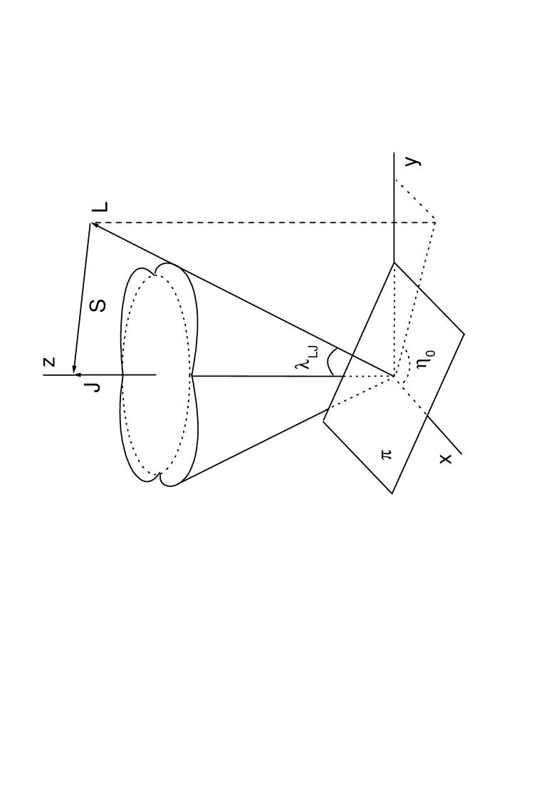
Figure 1: The orbital plane, $\pi$, tilts back and forth ( corresponding to ${\bf L}$ moves along the curves). ${\bf L}$, ${\bf S}$ and ${\bf J}$ form a triangle, in which ${\bf J}$ is invariable both in magnitude and direction; ${\bf L}$ varies in direction only; and ${\bf S}$ varies both in magnitude and direction

The change of $\lambda_{LJ}$ also means the orbital plane tilts back and forth, as shown in Fig 1, in turn both $\lambda_{LS}$ and $\lambda_{JS}$ vary with time. Therefore, by Eq(6), the derivative of the rate of orbital precession can be given by,

$$\dot{\Omega}_{0}=\Omega_{2}\Omega_{12}X_{3}X_{4}-\Omega_{12}X_{1}(\Omega_{01}X_{2}+\Omega_{12}X_{3})\ \,,$$ (8)

where $\Omega_{12}=\Omega_{1}-\Omega_{2}$, $\Omega_{01}=\Omega_{1}-\Omega_{0}$, $X_{1}=\frac{S^{\parallel}_{1}}{S}\sin\lambda_{LS_{1}}$, $X_{2}=\tan\eta_{ss1}$, $X_{3}=\frac{S_{V1}S_{V2}}{S^{2}}\frac{\sin\eta_{s1s2}}{\alpha\sin\lambda_{JS}}$, and $X_{4}=\frac{\cos^{2}\lambda_{LS}}{\sin\lambda_{LS}}$; with $\alpha=\sin\lambda_{JS}+\frac{\cos^{2}\lambda_{LS}}{\sin\lambda_{LS}}$, $S_{V1}=S_{1}\sin\lambda_{JS1}$ and $S_{V2}=S_{2}\sin\lambda_{JS2}$ represent components of $\bf{S}_{1}$ and $\bf{S}_{2}$ that are vertical to $\bf{J}$.

Note that $\Omega_{1}$ and $\Omega_{2}$ are unchanged, and $\lambda_{LS_{\alpha}}$ are unchanged, since they decay much slower than that of the orbitapo . The second derivative of $\Omega_{0}$ are given by,

$$\ddot{\Omega}_{0}=\Omega_{2}\Omega_{12}(\dot{X}_{3}X_{4}+X_{3}\dot{X}_{4})-\Omega_{12}\dot{X}_{1}(\Omega_{01}X_{2}+\Omega_{12}X_{3})$$

$$-\Omega_{12}X_{1}(\Omega_{01}\dot{X}_{2}+\Omega_{12}\dot{X}_{3})\ \,,$$ (9)

where $\dot{X}_{\alpha}$ is the first derivative of ${X}_{\alpha}$. $\dddot{\Omega}_{0}$ can be easily obtained from Eq(9).

$\dot{\Omega}_{0}$, the derivative of $\Omega_{0}$, can be absorbed by $\dot{P}_{b}$. The variation in the precession velocity of the orbit results in a variation of orbital frequency (${\nu}_{b}=2\pi/P_{b}$), ${\nu}^{\prime}_{b}-{\nu}_{b}=\dot{\Omega}_{0}\Delta t$, then we have $\dot{\nu}_{b}=\dot{\Omega}_{0}$ and $\ddot{\nu}_{b}=\ddot{\Omega}_{0}$, therefore,

$$\dot{P}_{b}=-\frac{\dot{\Omega}_{0}P_{b}^{2}}{2\pi}\ \,,\ \ \ \ \ddot{P}_{b}=-\frac{\ddot{\Omega}_{0}P_{b}^{2}}{2\pi}-\frac{\dot{\Omega}_{0}P_{b}\dot{P}_{b}}{\pi}\,.$$ (10)

From Eq(8) and Eq(10), we can see that the contribution of the orbital precession to $\dot{P}_{b}$ is 1 PPN, which is much larger than the contribution of GR to $\dot{P}_{b}$. Since it depends on parameters, $X_{1}$, $X_{2}$, $X_{3}$, and $\lambda_{LS}$ of Eq(8), then it is also possible that the geodetic precession induced $\dot{P}_{b}$ is comparable to, or even smaller than the prediction of GR in special cases (special combination of $\lambda_{LS}$, $\lambda_{LS1}$, $\eta_{SS1}$ and $S_{1}/S$).

The effect of S-L coupling on secular evolution of the orbital inclination, $i$, can be given as,

$$\cos i=\cos\lambda_{LJ}\cos I-\sin\lambda_{LJ}\sin I\cos\eta_{0}\ \,,$$ (11)

where $I$ is the angle between the total angular momentum, ${\bf J}$, and LOS, and $\eta_{0}=\Omega_{0}t+\eta_{i}$ ($\eta_{i}$ is the initial phase) is the phase of precession of ${\bf L}$. Thus $i$ is also a function of time. By Eq(11) we have,

$$di/dt=-\frac{\Omega_{0}S}{L}\sin\eta_{0}+O(r^{-7/2})\ \,.$$ (12)

Thus all parameters that are related with the orbital inclination will change with the geodetic precession. Hence the projected semi-major axis, $x=a_{1}\sin i/c$, will vary as the precession of the orbital plane. By Eq(12), the derivatives of the projected semi-major axis are

$$\dot{x}=-x\Omega_{0}\sin\lambda_{LJ}\sin\eta_{0}\cot i\ \,,$$ (13)

$$\ddot{x}=-\dot{x}(\dot{\Omega}_{0}/\Omega_{0}+\Omega_{0}\cot\eta_{0})\ \,.$$ (14)

As discussed between Eq(7) and Eq(8), the change of $S$ leads to the change of $\Omega_{0}$, and in turn $\dot{P}_{b}$ and $\ddot{P}_{b}$. If there is only one spin, then $S$ is a constant, thus there will be only a static addition (${\Omega}_{0}=const$) to the apsidal motion, as shown in Eq(7). In this case, the orbital precession is also static, which will only cause a variation in $\dot{x}$, as shown in Eq(13), whereas, $\dot{P}_{b}$ and $\ddot{P}_{b}$ are not influenced at all ($\dot{\Omega}_{0}=0$ and $\ddot{\Omega}_{0}=0$). This is why the quadrupole-orbit model (also the one spin S-L coupling model) cannot explain $\dot{P}_{b}$ and $\ddot{P}_{b}$ in PSR J2051$-$0827 and PSR B1957$+$20.

IV effects of geodetic precession induced $\Omega_{0}$

The S-L coupling induced $\Omega_{0}$ leads to the precession of the orbital plane, then the orbital inclination, $i$, varies, as in Eq(12), and in turn the projected semi-major axis, $\dot{x}$, varies, as in Eq(13). Comparing the predicted $\dot{x}$ with the observational $\dot{x}^{obs}$, we can constrain the angle $\lambda_{LJ}\approx S/L$, and therefore the moment of the inertia of the pulsar.

IV.1 PSR J2051$-$0827

The measured orbital period derivatives of PSR J2051$-$0827do are list in Table I, the derivatives of the semi-major axis are $\dot{x}^{obs}=-23(3)\times 10^{-14}$ and $\ddot{x}^{obs}=7(15)\times 10^{-22}$ s^-1. The measured ones are much larger than the corresponding predictions of GR, $\dot{P}_{b}^{GR}=-3.8\times 10^{-14}$ and $\dot{x}^{GR}=-1.3\times 10^{-19}$, as well as the proper motion induced effects, $\dot{x}^{pm}=4(2)\times 10^{-17}$ko .

With $m_{1}=1.40M_{\odot}$, $m_{2}=0.03M_{\odot}$ and ${P}_{b}=0.09911$ddo , we have the semi-major axis, $a=(GM/\nu_{b}^{2})^{1/3}=7.08\times 10^{10}$ cm, and orbital angular momentum, $L=\nu_{b}\mu a^{2}(1-e^{2})^{1/2}=2.17\times 10^{50}$g cm²s^-1, with $\mu$ the reduced mass. From Eq(2), we have $\Omega_{2}=3.25\times 10^{-9}$s^-1, and from Eq(6), $|\Omega_{0}|\approx\Omega_{2}\approx 3\times 10^{-9}$s^-1. With $x=x^{obs}=0.045052$, $|\dot{x}^{obs}|=2.3\times 10^{-13}$, Eq(13) becomes

$$0.045\times(3\times 10^{-9})\sin\lambda_{LJ}|\sin\eta_{0}\cot i|=2.3\times 10^{-13}\,.$$ (15)

Thus $\sin\lambda_{LJ}|\sin\eta_{0}\cot i|\approx 2\times 10^{-3}$. If $|\sin\eta_{0}\cot i|\approx 1\times 10^{-1}$, then $\lambda_{LJ}\approx 2\times 10^{-2}$, which means $S/L\approx 2\times 10^{-2}$. With $L$ obtained above, we have $S_{1}\approx S\approx 4\times 10^{48}$g cm²s^-1. Having the measured pulsar period, $P=4.50864$ms, the moment of inertia of the pulsar is $I_{1}\approx 3\times 10^{45}$g cm².

IV.2 PSR B1957$+$20

The negative orbital period derivative changes to positive during the observation of PSR B1957$+$20aft . The measured derivatives of the orbital period are shown in Table 2. The measured upper-limit to $\dot{x}$ is $\dot{x}^{obs}<3\times 10^{-14}$. The measured ones are also much larger than the corresponding GR predictions, $\dot{P}_{b}^{GR}=-3.4\times 10^{-15}$ and $\dot{x}^{GR}=-6.1\times 10^{-21}$, as well as the proper motion induced effect, $\dot{x}^{pm}=2.4\times 10^{-16}$ko .

Similarly, with $m_{1}=1.40M_{\odot}$, $m_{2}=0.025M_{\odot}$ and ${P}_{b}=33001.91484$saft , we have $a=1.74\times 10^{11}$ cm, $L=2.82\times 10^{50}$g cm²s^-1, $\Omega_{2}=3.43\times 10^{-10}$s^-1, and in turn $|\Omega_{0}|\approx\Omega_{2}\approx 3\times 10^{-10}$s^-1. From Eq(13), with $x=x^{obs}=0.0892253$ and $|\dot{x}^{obs}|<3\times 10^{-14}$, we have

$$0.089\times(3\times 10^{-10})\sin\lambda_{LJ}|\sin\eta_{0}\cot i|<3\times 10^{-14}\ \,,$$ (16)

which leads to , $\sin\lambda_{LJ}|\sin\eta_{0}\cot i|<1\times 10^{-3}$. If $|\sin\eta_{0}\cot i|\approx 1\times 10^{-1}$, then $\lambda_{LJ}<1\times 10^{-2}$. Which means $S/L<1\times 10^{-2}$, and by the obtained $L$, we have $S_{1}\approx S<3\times 10^{48}$g cm²s^-1. Finally, with the measured pulsar period, $P=1.607$ms, the moment of inertia of the pulsar is $I_{1}<8\times 10^{44}$g cm² .

The simple estimation above indicates that PSR B1957$+$20 has similar moment of inertia as that of PSR J2051$-$0827.

In these two estimations, the assumptions $|\Omega_{0}|\approx\Omega_{2}$ and $|\sin\eta_{0}\cot i|\approx 1\times 10^{-1}$ are used. Consider the deviation of these two assumptions from the corresponding true values, the most likely moment of inertia from the observational constraints is about $10^{44}$g cm²–$10^{45}$g cm².

V effects of geodetic precession induced $\dot{\Omega}_{0}$, $\ddot{\Omega}_{0}$, $\dddot{\Omega}_{0}$

From Eq(8) and Eq(9), we can see that $\dot{\Omega}_{0}$, $\ddot{\Omega}_{0}$ and $\dddot{\Omega}_{0}$ can vary in wider and wider range, which can be written approximately as (for the convenience of estimation),

$$|\dot{\Omega}_{0}|\approx c_{1}\Omega_{2}^{2}\ \,,\ \ |\ddot{\Omega}_{0}|\approx c_{2}\Omega_{2}^{3}\ \,,\ \ |\dddot{\Omega}_{0}|\approx c_{3}\Omega_{2}^{4}\ \,,$$ (17)

where $c_{1}$ represents the contribution of $X_{\alpha}$ to $\dot{\Omega}_{0}$, $c_{2}$ corresponds to the contribution of $X_{\alpha}$ and $\dot{X}_{\alpha}$ to $\ddot{\Omega}_{0}$, and $c_{3}$ corresponds to the contribution of $X_{\alpha}$, $\dot{X}_{\alpha}$ and $\ddot{X}_{\alpha}$ to $\dddot{\Omega}_{0}$. Obviously $\dddot{\Omega}_{0}$ can vary in a wider range than $\ddot{\Omega}_{0}$, and $\ddot{\Omega}_{0}$ can vary in a wider range than $\dot{\Omega}_{0}$.

For PSR J2051$-$0827, $\Omega_{2}^{2}\approx 9.8\times 10^{-18}$s^-2, $\Omega_{2}^{3}\approx 3.2\times 10^{-26}$s^-3 and also (equation not shown) $\Omega_{2}^{4}\approx 1.0\times 10^{-34}$s^-4. Assuming $c_{1}=c_{2}=c_{3}=0.2$, and by Eq(17) and Eq(10), the derivatives of $P_{b}$ can be obtained, $|\dot{P}_{b}|\approx 2\times 10^{-11}$, $|\ddot{P}_{b}|\approx 8\times 10^{-20}$s^-1 and $|\dddot{P}_{b}|\approx 2\times 10^{-28}$s^-2. Which can be well consistent with the corresponding observations, as shown in Table I.

For PSR B1957$+$20, the measured derivatives of ${P}_{b}^{obs}$ is larger than that of PSR J2051$-$0827. By assuming $c_{1}=1$, $c_{2}=1\times 10^{3}$ and $c_{3}=1\times 10^{4}$, and through the same treatment, we have $|\dot{P}_{b}|\approx 2\times 10^{-11}$, $|\ddot{P}_{b}|\approx 7\times 10^{-18}$s^-1 and $|\dddot{P}_{b}|\approx 2\times 10^{-26}$s^-2, which can be consistent with the corresponding observations, as shown in Table II.

It is likely that in PSR B1957$+$20 the magnitude of $S_{1}$ and $S_{2}$ are close, so that $S$ can be small, which leads to a large ${X}_{\alpha}$, and in turn large derivatives of ${P}_{b}$ as shown in Eq(6) and Eq(8)-Eq(10).

VI discussion and conclusion

Geodetic precession induced pulsar spin in binary pulsar PSR B1913+16 has been studied through structure parameters of pulsar profilekr ; wt . Actually the variation of pulsar spin axis (former) and the measured secular variabilities discussed in this paper are induced by the same physics underlying in binary pulsar systems, S-L coupling. The former corresponds to the reaction of the pulsar spin to the torque in the S-L coupling; while the latter corresponds to reaction of the orbit to the same torque.

By adding one more spin into the S-L coupling of Apostolatos et al and Kidderapo ; kid , we establish the relationship among the secular variability, geodetic precession and moment of inertia of binary pulsars. The new model provides: (a) a unified model that explain both $\dot{x}$ and $\dot{P}_{b}$, which has been interpreted separately by different models, (b) a new method which can extract the moment of inertia through pulsar timing measurement, (c) a new test of the geodetic precession which has strong effects to pulsar timing.

Table 1: Measured parameters compare with the geodetic precession induced ones in PSR J2051$-$0827

observations	predictions
$\dot{x}^{obs}=-23(3)\times 10^{-14}$	$|\dot{x}|\approx 2\times 10^{-13}$ a
$({\ddot{x}}/{\dot{x}})^{obs}\lesssim-3.0\times 10^{-9}$s-1	$|{\ddot{x}}/{\dot{x}}|\approx 3\times 10^{-9}$s-1 b
$\dot{P}_{b}^{obs}=-15.5(8)\times 10^{-12}$	$|\dot{P}_{b}|=|\frac{\dot{\Omega}_{0}P_{b}^{2}}{2\pi}|\approx 2\times 10^{-11}$
$\ddot{P}_{b}^{obs}=2.1(3)\times 10^{-20}$s-1	$|\ddot{P}_{b}|\approx|\frac{\ddot{\Omega}_{0}P_{b}^{2}}{2\pi}|\approx 8\times 10^{-20}$s-1
$\dddot{P}_{b}^{obs}=3.6(6)\times 10^{-28}$s-2	$|\dddot{P}_{b}|\approx|\frac{\dddot{\Omega}_{0}P_{b}^{2}}{2\pi}|\approx 2\times 10^{-28}$s-2

We assume $c_{1}=c_{2}=c_{3}=0.2$ in Eq(17). ^a $|\dot{x}|$ is given by Eq(15), and ^b $\ddot{x}/\dot{x}$ is given by Eq(14).

Table 2: Measured parameters compare with the geodetic precession induced ones in PSR B1957$+$20

observations	predictions
$|\dot{x}|^{obs}<3\times 10^{-14}$	$|\dot{x}|\lesssim 3\times 10^{-14}$ a
$\dot{P}_{b}^{obs}=1.47(8)\times 10^{-11}$	$|\dot{P}_{b}|=|\frac{\dot{\Omega}_{0}P_{b}^{2}}{2\pi}|\approx 2\times 10^{-11}$
$\ddot{P}_{b}^{obs}=1.43(8)\times 10^{-18}$s-1	$|\ddot{P}_{b}|\approx|\frac{\ddot{\Omega}_{0}P_{b}^{2}}{2\pi}|\approx 7\times 10^{-18}$s-1
$|\dddot{P}_{b}|^{obs}<3\times 10^{-26}$s-2	$|\dddot{P}_{b}|\approx|\frac{\dddot{\Omega}_{0}P_{b}^{2}}{2\pi}|\approx 2\times 10^{-26}$s-2

We assume $c_{1}=1$, $c_{2}=1\times 10^{3}$, and $c_{3}=1\times 10^{4}$ in Eq(17). ^a $|\dot{x}|$ is given by Eq(16).

References

- (1) B.M. Barker, and R.F. O’Connell, Phys. Rev. D, 12, 329-335 (1975).
- (2) L.L. Smarr, and R.D. Blandford, Astrophys.J. 207, 574-588 (1976).
- (3) D. Lai, L. Bildsten, and V. Kaspi, Astrophys.J. 452, 819-824 (1995).
- (4) N. Wex, and S.M. Kopeikin, Astrophys J., 514, 388 (1999).
- (5) A.J.S. Hamilton, and C.L.Sarazin, Mon.Not.R.astro. Soc, 198, 59-70 (1982).
- (6) T.A. Apostolatos, C. Cutler, J.J. Sussman, and K.S. Thorne, Phys. Rev. D, 49,6274-6297 (1994).
- (7) L.E. Kidder, Phys. Rev. D, 52, 821-847 (1995).
- (8) Z. Arzoumanian, A.S. Fruchter, and J.H. Taylor, Astrophys. J 426, L85-L88 (1994).
- (9) O. Doroshenko, O. Löhmer, M. Kramer, A. Jessner, R. Wielebinski, A.G. Lyne, and Ch. Lange Astro-Astrophys, 379, 579-588 (2001).
- (10) J.H. Applegate, and J. Shaham, Astrophys J. 436, 312-318 (1994).
- (11) S.M. Kopeikin, Astrophys. J 467, L93-L95 (1996).
- (12) M. Kramer, Astrophys.J. 509, 856-860 (1998).
- (13) J.M. Weisberg, and J.H. Taylor, Astrophy. J. 576, 942-949 (2002).