A photometric monitoring of bright high-amplitude $\delta$ Scuti stars

We present new photometric data for seven high-amplitude $\delta$ Scuti stars. The observations were acquired between 1996 and 2002, mostly in the Johnson photometric system. For one star (GW UMa), our observations are the first since the discovery of its pulsational nature from the Hipparcos data.The primary goal of this project was to update our knowledge on the period variations of the target stars. For this, we have collected all available photometric observations from the literature and constructed decades-long O$-$C diagrams of the stars. This traditional method is useful because of the single-periodic nature of the light variations. Text-book examples of slow period evolution (XX Cyg, DY Her, DY Peg) and cyclic period changes due to light-time effect (LITE) in a binary system (SZ Lyn) are updated with the new observations. For YZ Boo, we find a period decrease instead of increase. The previously suggested LITE-solution of BE Lyn (Kiss & Szatmáry 1995) is not supported with the new O$-$C diagram. Instead of that, we suspect the presence of transient light curve shape variations mimicking small period changes.

1 Introduction

High-amplitude $\delta$ Scuti stars (hereafter HADSs) are either Pop. I stars close to the main sequence or evolved Pop. II stars (these are also known as SX Phe variables) with very characteristic light variations caused by radial pulsations (Rodríguez et al. 1996). Typical periods range from 0$\aas@@fstack{d}$05 to 0$\aas@@fstack{d}$15 associated with relatively large amplitudes ($A_{\rm V}\geq 0\aas@@fstack{m}30$ is a widely adopted convention). Owing to their short periods and high amplitudes, these stars are very good targets for small and moderate-sized telescopes, so that interesting astrophysical phenomena can be easily studied even with modest instrumentation. Apart from attempts to detect evolutionary effects, the most interesting case studies are related to the suspected binary HADSs, in which the physical parameters of the pulsating component can be constrained from the binary nature. However, the time-span of the available observations is often too short, therefore, significant observational efforts have to be done to reach unambiguous conclusions.

In Paper I (Kiss et al. 2002b) we discussed the double-mode pulsation of V567 Ophiuchi. The aims of this project have been outlined in Kiss et al. (2002b) and to avoid repetition, we refer to theoretical and observational aspects discussed in that paper. The main aim of this paper is to publish a new dataset for seven variable stars. Besides the new photometric data we give an updated description of their period changing behaviour. The analysis of multicolour data in terms of physical parameters will be published in the final paper of the series (Derekas et al., in prep.).

The structure of the paper is the following. Target selection and observations are described in Sect. 2. The main part of the paper is Sect. 3, in which the results are presented. Separate subsections are devoted to individual stars, where every relevant detail (observational data, sample light curves, updated O$-$C diagrams) is given. A brief summary is presented in Sect. 4.

2 Target selection and instrumentation

The observations were started with regular monitoring of BE Lyncis, for which we suspected binarity (Kiss & Szatmáry 1995). The first extension was made toward XX Cygni (Kiss & Derekas 2000) and since then, we have tried to include all HADSs in the northern sky brighter than $V=11\aas@@fstack{m}3$ at maximum (this limit was determined by the typical accuracy and limiting magnitudes of our main instruments). Unfortunately, this goal was unreachable because of unfavourable weather conditions in several observing seasons. That is why we excluded the following bright northern HADSs: GP And, AD CMi, DH Peg, V1719 Cyg. Also, we concentrated on the monoperiodic variables and some of these excluded stars are well-known double-mode pulsators (see Rodríguez et al. 1996). Thus, our sample consisted of 10 variables, however, two stars (V1162 Ori and DE Lac) had so meagre coverage that we had to remove them from the final target list. V567 Oph turned to be a double-mode pulsator and was discussed in Kiss et al. (2002b). The remaining seven HADSs are listed in Table 1, where their main observational properties are also summarized.

Table 1: The list of programme stars. The magnitude ranges and periods are taken from the GCVS.

Star	Pop.	$V_{\rm max}$	$V_{\rm min}$	P (d)	Type of obs.
DY Her	I	10$\aas@@fstack{m}$15	10$\aas@@fstack{m}$66	0.14863	$V$
YZ Boo	I	10$\aas@@fstack{m}$30	10$\aas@@fstack{m}$80	0.10409	$V$
XX Cyg	II	11$\aas@@fstack{m}$28	12$\aas@@fstack{m}$13	0.13486	$V(RI)_{C}$
SZ Lyn	I	9$\aas@@fstack{m}$08	9$\aas@@fstack{m}$72	0.12053	$V$
BE Lyn	I	8$\aas@@fstack{m}$60	9$\aas@@fstack{m}$00	0.09587	$BV/uvby$
DY Peg	II	9$\aas@@fstack{m}$95	10$\aas@@fstack{m}$62	0.07293	$BV/uvby$
GW UMa	II?	9$\aas@@fstack{m}$48	9$\aas@@fstack{m}$97	0.20319a	$BVI_{C}$

^a ESA (1997)

During the seven years of observations, we have utilized various instrumentations at three observatories (Szeged Observatory, Piszkéstető Station of the Konkoly Observatory, Sierra Nevada Observatory). In the following we briefly introduce the telescopes and detectors used in this project. As the primary aim was to obtain good light curve coverage enabling accurate determination of the epochs of maximum, the CCD measurements were uninterrupted single-filtered $V$-band observations, with a few exceptions.

• Szeged Observatory, 0.28m Schmidt-Cassegrain (Sz28)

  This telescope is located in the very centre of the city of Szeged, thus suffering from strong light pollution. For our observations on two nights in 2002, it was equipped with an SBIG ST–7I CCD camera (765$\times$510 9$\mu$m pixels giving a field of view (FOV) of 11$\aas@@fstack{\prime}$5$\times$7$\aas@@fstack{\prime}$5). This instrument was the least used in our project.

• Szeged Observatory, 0.4m Cassegrain (Sz40)

  The majority of the observations were acquired with the 0.4m Cassegrain-telescope of the Szeged Observatory. Between 1996 and 2000, photoelectric photometry was carried out through Johnson $BV$ filters. The detector was an SSP–5A photoelectric photometer and we obtained differential photometric data using selected comparison stars located near to target stars. The photometer was replaced by an SBIG ST–9E CCD camera in 2001 (512$\times$512 20$\mu$m pixels, FOV=$6^{\prime}\times 6^{\prime}$) and most single-filtered $V$-band observations were made with this instrument.

• Piszkéstető, 0.6m Schmidt (P60)

  Fewer observations were done with the 60/90/180cm Schmidt-telescope mounted at the Piszkéstető Station of the Konkoly Observatory. The detector was a Photometrics AT200 CCD camera (1536$\times$1024 9$\mu$m pixels, FOV$=28^{\prime}\times 19^{\prime}$). The observations were done either in $B$ or $V$ filters.

• Sierra Nevada Observatory, 0.9m Ritchey-Chrétien (SNO90)

  Occasionally, we acquired simultaneous $uvby$ Strömgren photometric observations using the 0.9m telescope of the Sierra Nevada Observatory (Spain) equipped with a six-channel Strömgren-Crawford spectrograph photometer.

The data were reduced in a standard fashion. For the photoelectric observations, we made use of different computer programs written by LLK, which were based on methods described in Henden & Kaitchuk (1982). The CCD observations were reduced with standard tasks in IRAF, including bias removal and flat-field correction utilizing sky-flat images taken during the evening or morning twillight. Differential magnitudes were calculated with aperture photometry using two comparison stars of similar brightnesses. We have not tried PSF photometry because the small FOVs contained too few stars for a reliable PSF-determination (see Vinkó et al. 2003 for a related discussion using the same instruments). The typical photometric accuracy was $\pm 0\aas@@fstack{m}01-0\aas@@fstack{m}02$, depending on the weather conditions and brightness difference of the variable and comparison stars. In fields far from the galactic plane – e.g. those of BE Lyn and SZ Lyn – we had to choose somewhat fainter comparisons, typically 2–3 mags dimmer than the target, which consequently increased the noise level of the data.

Thanks to the dense sampling of the light curves, new times of maximum light were easy to determine from the individual cycles. This was done by fitting low-order (3–5) polynomials to the light curves around maxima. We repeated the fitting procedure by changing the parameters of the fits to yield some insights into the uncertainty range of the determined epochs. We estimate the typical accuracy as $\pm$0$\aas@@fstack{d}$0003 (i.e. $\pm$26 sec), which is comparable with the usual exposure lengths.

3 Results

The period variations were studied with the classical O$-$C (observed minus calculated) method. The use of this simple approach is justified by the remarkable stability of the HADS light curves, both in amplitude (Rodríguez 1999) and in period (Rodríguez et al. 1995, Breger & Pamyatnykh 1998, hereafter BP98). The blind use of the O$-$C technique has been strongly criticised by Lombard and Koen in their series of papers (e.g. Lombard & Koen 1993, Koen & Lombard 1995, Koen 1996, Lombard 1998) underlining the importance of the evaluation of the model residuals. For this, they developed various statistical methods by analysing autocorrelation of the residuals. This is a crucial point when studying long-period stars (e.g. Mira variables) with relatively large stochastic scatter of the period. In case of the HADSs one does not expect such intrinsic period scatter (as suggested by the observations) and evolutionary period changes might be constrained with the O$-$C technique.

Nevertheless, in every case we have checked the model residuals via their frequency analysis. This can be used to search for secondary periodicity or slow changes of the period hidden by the observational scatter. The basic idea is the fact that a small modulation of the O$-$C diagram appears as an additional periodicity of the O$-$C residuals. A recent example for this has been given by Pócs et al. (2002), who presented the Fourier spectrum of the O$-$C diagram of the multiply periodic HADS RV Ari, clearly revealing $f_{\rm m}=f_{1}-f_{0}$ in their data. On the other hand, if there is a slight period change in the data and a wrong model is subtracted, then the residuals’ spectrum will show a peak very close to $f={1\over P}$. This closely separated peak in the Fourier spectrum, however, can be explained by another way, too: it appears simply because of the periodicity of the spectrum itself. The Fourier transform of an O$-$C diagram is periodic with the frequency of the ephemeris because of the periodicity of data sampling. Therefore, if a long-term trend is present in the residuals, that causes a low-frequency component at $f_{\rm low}$, which appears again at $f_{\rm low}+f$. Whatever explanation we adopt, Fourier analysis of the residuals can help emphasize the hardly visible trends of the data.

3.1 DY Herculis

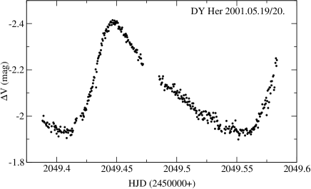
Figure 1: Sample light curve for DY Her.

The most recent period-change study for DY Her was made by Yang et al. (1993), but even the last data of that paper were obtained in 1984. Previously, Szeidl & Mahdy (1981) collected all available data to study long-term period variations. Both studies revealed a slow period decrease of the star. The main characteristics are summarized by Peña et al. (1999). Recently, Pócs & Szeidl (2000) interpreted the long-term O$-$C diagram in terms of the light-time effect (LITE) caused by a hypothetical low-mass component, although their conclusions were quite ambiguous.

We observed the star on four nights in 2001 with Sz40. More than 2000 individual exposures of 20–40 seconds were obtained in $V$-band. Two comparison stars located within 6^′ were used (comp=GSC 0968-1532, check=GSC 0968-1002, both stars are about 11$\aas@@fstack{m}$0). The full log is given in Table 2, a sample light curve is shown in Fig. 1. There is no new time of maximum for the first night, because we had to interrupt our observations for half an hour and the maximum just appeared during that break.

Table 2: Journal of observations and new times of maximum for DY Her

Date	filter	Inst.	Points	$HJD_{\rm max}$
2001-05-09	$V$	Sz40	509	–
2001-05-10	$V$	Sz40	663	2452040.3804
				2452040.5317
2001-05-19	$V$	Sz40	409	2452049.4471
2001-06-25	$V$	Sz40	506	2452086.4579

We have collected all times of maximum from the literature (the updated list of references is given in Pócs & Szeidl 2000) to arrive to the final O$-$C diagram. It is plotted in Fig. 2 and was calculated with the following ephemeris:

$$HJD_{\rm max}=2433439.4871+0.1486309\times E$$

(the epoch is from the GCVS, the period from ESA 1997).

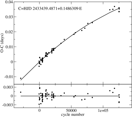
Figure 2: The O$-$C diagram of DY Her. The solid line shows the parabolic fit.

The parabolic fit has the form

$$O-C=-0.0001(2)+3.9(1)\times 10^{-7}E-8.3(11)\times 10^{-13}E^{2}$$

with an rms of 0$\aas@@fstack{d}$00115 ($\pm$errors of the last digits are in parentheses). The linear fit yields higher rms (0$\aas@@fstack{d}$00157) and the Fourier spectrum of the residuals (Fig. 3) shows that the parabolic residuals are closer to an uncorrelated noise. The peak in the spectrum of the linear residuals appears close to the pulsational frequency (with wich the O$-$C was calculated): the difference is $2.30\times 10^{-4}$ d^-1. Therefore, the hypothetical binary nature (Pócs & Szeidl 2000) of the star is not confirmed and we are confident about the definite detection of the slow period decrease. The parabolic coefficient (usually denoted as $\beta/2$=0.5 P dP/dt) results in a period change ${1\over P}{dP\over dt}=(-2.8\pm 0.4)\times 10^{-8}$ year^-1, which is slightly smaller and more accurate than the value used by BP98 ($-4\times 10^{-8}$ year^-1). Nevertheless, the main conclusion drawn by several earlier authors is not changed, as this smaller decreasing rate is generally in good agreement with the evolutionary calculations.

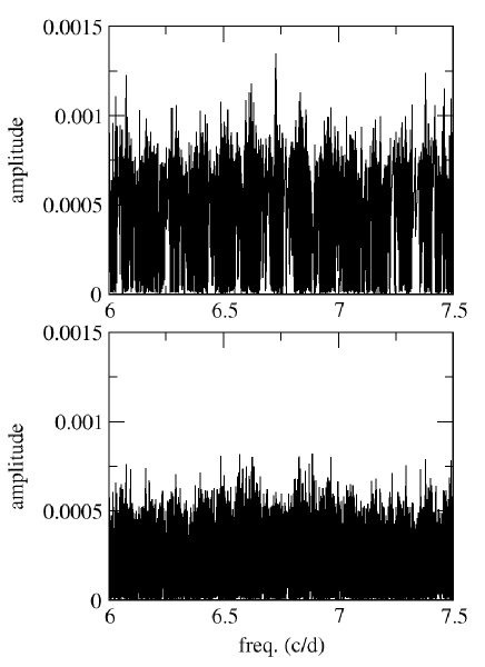
Figure 3: Top panel: the Fourier spectrum of the residuals for DY Her after subtracting a linear fit. Bottom panel: the same with the parabolic fit.

3.2 YZ Bootis

YZ Boo has quite a long observational record and the most relevant information on the star was summarized by Peña et al. (1999). Its period change was studied by Szeidl & Mahdy (1981), Jiang (1985) and Hamdy et al. (1986). The latter authors analysed the longest dataset available at that time and concluded that the O$-$C diagram can be fitted with a positive parabola, indicating a constant period increase. They arrived at a relative period changing rate of ${1\over P}{dP\over dt}=+3\times 10^{-8}$ year^-1.

Table 3: Journal of observations and new times of maximum for YZ Boo

Date	filter	Inst.	Points	$HJD_{\rm max}$
2001-03-16	$V$	Sz40	279	2451985.6116
2001-04-01	$V$	Sz40	536	2452001.5381
2001-04-25	$V$	Sz40	177	2452025.3695
2001-04-28	$V$	Sz40	697	2452028.3902
				2452028.4946
				2452028.5975
2001-04-30	$V$	Sz40	526	2452030.3693
				2452030.4726
				2452030.5759
2001-05-09	$V$	Sz40	307	2452039.3221

Our observations were carried out using Sz40 on six nights in 2001 (Table 3). The exposure time was between 15 and 40 s. Unfortunately, only one comparison star was available in the small FOV of the instrument (GSC 2569-1184 with $V\approx$11$\aas@@fstack{m}$3). Slightly more than 2500 data points were obtained. The longest subset, containing 697 points, is shown in Fig. 4.

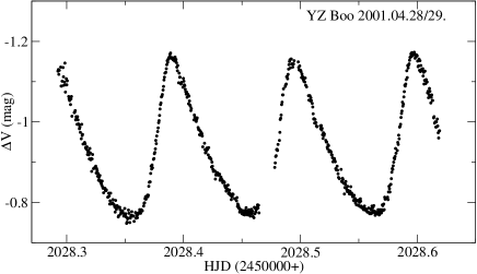
Figure 4: Sample light curve for YZ Boo.

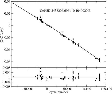
Figure 5: The O$-$C diagram of YZ Boo. The solid line denotes the parabolic fit. Residuals are shown below.

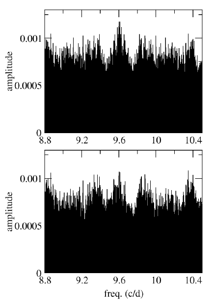
Figure 6: Top panel: Fourier spectrum of the residuals for YZ Boo after subtracting a linear fit. Bottom panel: the same with the parabolic fit.

Ten new times of maximum were determined from the individual light curves (Table 3), which extended the existing data by another $\sim$15 years. Published times of maximum were collected from Hamdy et al. (1986) and references therein, Kim & Joner (1994), Agerer et al. (1999) and Agerer & Hübscher (2000). The O$-$C diagram was calculated with the following ephemeris:

$$HJD_{\rm max}=2438206.6961+0.1040920\times E$$

and is plotted in Fig. 5. The solid line corresponds to the parabolic fit:

$$O-C=0.0018(2)-4.25(6)\times 10^{-7}E-1.5(6)\times 10^{-13}E^{2}$$

with an rms of 0$\aas@@fstack{d}$00169. The data can be fitted almost equally well with a simple linear term (rms=0$\aas@@fstack{d}$00173), but a frequency analysis of the residuals slightly favours continuous period change. It is shown in Fig. 6. There is a peak at $f\approx 9.6116$ d${}^{-1}(\approx{1\over P}+4.7\times 10^{-3}$ d^-1) in the spectrum of the residuals of the linear fit, while the spectrum of the parabolic residuals are more noise-like. This suggest a real period change over the six decades of observations, although the evidence is fairly weak.

If we accept its significance, the given second-order coefficient corresponds to a relative period changing rate ${1\over P}{dP\over dt}=(-1\pm 0.4)\times 10^{-8}$ year^-1, which has an absolute value of about one third of the previous estimate by Hamdy et al. (1986) and slightly larger than that of Peniche et al. (1985), but with the opposite sign. It means that contrary to Hamdy et al. (1986) and Peniche et al. (1985), we found period decrease instead of increase. The determined rate has great uncertainty and we recall a note by Peniche et al. (1985): “…it is impossible right now to decide if the period is constant or if it is varying, but this will be feasible only if the star is regularly observed during the next 40 years”. Almost 20 years have passed since then and the uncertainty is still too large. That clearly shows the need for continuous follow-up in the future. The given slow rate is in good agreement with theoretical calculations of BP98, which predict small period changes of the same order of magnitude.

3.3 XX Cygni

Our unfiltered observations were published in Kiss & Derekas (2000). Recently, XX Cygni has been revisited by Zhou et al. (2002) and Blake et al. (2003). The history and observational record of XX Cyg can be found in those papers. Contrary to our earlier conclusion, these authors provided convincing arguments for slow continuous period increase with at a rate of about ${1\over P}{dP\over dt}=+1.13\times 10^{-8}$ year^-1 (Blake et al. 2003) and $0.94\times 10^{-8}$ year^-1 (Zhou et al. 2002). Here we add one night of observations carried out in 2002. The comparison stars were the same as in Kiss & Derekas (2000).

Table 4: Journal of observations and new times of maximum for XX Cyg

Date	filter	Inst.	Points	$HJD_{\rm max}$
2002-07-20	$V$	Sz40	60	2452476.4983
2002-07-20	$R_{\rm C}$	Sz40	61	2452476.4982
2002-07-20	$I_{\rm C}$	Sz40	59	2452476.4976

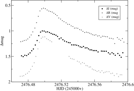
Figure 7: $V(RI)_{\rm C}$ light curves of XX Cyg.

The obtained light curves are plotted in Fig. 7, while the determined epochs of maximum are shown in Table 4. The mean O$-$C value with the ephemeris from Szeidl & Mahdy (1981) is $+0\aas@@fstack{d}0079$ which falls close to any recent prediction. The light curve shape is similar to the ones shown in Blake et al. (2003) and a well-expressed post-maximum bump is present in the $R$-band data. Only weak evidence is present for the possible transient secondary maximum that is discussed in Blake et al. (2003): there is a slight hump around HJD 2452476.54 which resembles that of in Fig. 2 of Blake et al. (2003) but no conclusive remark can be given based on this.

3.4 SZ Lyncis

SZ Lyncis is the best documented example of a binary pulsating star with very clear light-time effects. The period variations of the star were studied by Paparó et al. (1988) and Moffett et al. (1988). Since then it has been totally neglected and no new times of maximum have appeared in the literature, except the one by the Hipparcos satellite.

We observed SZ Lyn with two telescopes on four nights in 2001. The exposure times were between 15 and 120 seconds, depending on the instrument and weather conditions. Two nearby stars were chosen as comparisons (comp = GSC 2979-1329, $V\approx 10\aas@@fstack{m}5$, check = GSC 2979-1343, $V\approx 10\aas@@fstack{m}8$). More than 1500 individual points have been acquired (Table 5) and a sample light curve is shown in Fig. 8.

Table 5: Journal of observations and new times of maximum for SZ Lyn

Date	filter	Inst.	Points	$HJD_{\rm max}$
2001-02-25	$V$	P60	395	2451966.5244
2001-02-26	$V$	P60	239	2451967.3683
2001-04-03	$V$	Sz40	287	2452003.4072
2001-05-02	$V$	Sz40	619	2452032.3351

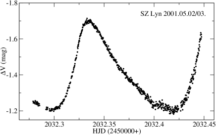
Figure 8: Sample light curve for SZ Lyn.

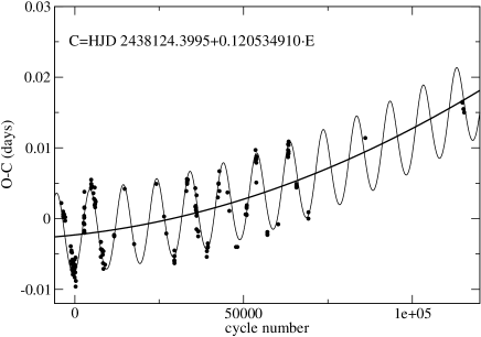
Figure 9: The O$-$C diagram of SZ Lyn. The thick solid line shows the parabolic part of the fit.

The four new times of maximum supplemented with the Hipparcos epoch (HJD 2448500.0560, ESA 1997) were added to the list of maxima (Paparó et al. 1988, Moffett et al. 1988). The resulting O$-$C diagram is plotted in Fig. 9. It was calculated with the ephemeris

$$HJD_{\rm max}=2438124.39955+0.120534910\times E$$

taken from Paparó et al. (1988). Our new observations confirm the consistent picture of the light-time effect thoroughly discussed in Paparó et al. (1988) and Moffett et al. (1988). The parabolic and light-time fit resulted in essentially the same parameters as those of the mentioned papers, which is not surprising, as the overwhelming majority of the fitted data is the same. We could, however, improve the value of the orbital period, which turned out to be $P_{\rm orb}=1190\pm 5$ d (contrary to 1177$\aas@@fstack{d}$7 and 1181$\aas@@fstack{d}$1 by Paparó et al. 1988 and Moffett et al. 1988, respectively). On the other hand, we derived a slightly smaller period changing rate of ${1\over P}{dP\over dt}=(+5\pm 1.8)\times 10^{-8}$ year^-1. We note that the quadratic term is still too uncertain. We have experimented with different averaging of the original O$-$C points to decrease the effects of the unequal data distribution. Different binnings changed a lot the parabolic coefficient (almost by a factor of two), and that marks a certain limit in the data interpretation.

3.5 BE Lyncis

Kiss & Szatmáry (1995) suspected binarity of BE Lyn, based on the seemingly cyclic O$-$C diagram. In order to confirm this preliminary result, we have continuously monitored this star since then. Previous observations are summarized in Rodríguez (1999), who did not find any long-term amplitude change of the light curve.

Table 6: Journal of observations and new times of maximum for BE Lyn. The first five epochs were re-determined from the observations in Kiss & Szatmáry (1995). For multicolour observations we only list epochs based on $V$-band data (either from Johnson or Strömgren photometry).

Date	filter	Inst.	Points	$HJD_{\rm max}$	Date	filter	Inst.	Points	$HJD_{\rm max}$
1995-01-31	$BV$	Sz40	267	2449749.4651	1999-03-08	$BV$	Sz40	172	2451246.2747
				2449749.5622					2451246.3704
				2449749.6562					2451246.4674
1995-02-05	$UBV$	Sz40	48	2449754.3545	1999-03-08	$uvby$	SNO90	62	2451246.3702
1995-02-13	$UBV$	Sz40	63	2449762.4075					2451246.4675
1996-01-31	$BV$	Sz40	51	2450114.5363	1999-04-24	$uvby$	SNO90	60	2451293.3477
1996-02-25	$BV$	Sz40	60	2450139.4639					2451293.4437
1996-02-26	$BV$	Sz40	60	2450140.4208	1999-04-25	$uvby$	SNO90	18	–
1997-02-20	$BV$	Sz40	75	2450500.5075	1999-05-12	$uvby$	SNO90	56	2451311.4673
1998-01-30	$BV$	Sz40	114	2450844.3906	1999-05-14	$uvby$	SNO90	37	2451313.4802
				2450844.4860	2000-02-10	$BV$	Sz40	57	2451585.3663
1999-01-26	$uvby$	SNO90	99	2451205.5313	2001-01-19	$uvby$	SNO90	33	2451929.4424
				2451205.6277					2451929.5377
				2451205.7231	2001-02-24	$B$	P60	215	2451965.2974
1999-02-27	$BV$	Sz40	234	2451237.2625	2001-02-24	$V$	P60	830	2451965.3927
				2451237.3596					2451965.4896
				2451237.4552	2001-03-14	$V$	Sz40	224	–
				2451237.5500	2001-03-16	$V$	Sz40	438	2451985.3329
1999-03-01	$BV$	Sz40	149	2451239.3712					2451985.5235
				2451239.4684	2001-12-08	$V$	Sz40	193	2452252.5191
1999-03-02	$uvby$	SNO90	305	2451240.4268	2002-04-06	$V$	Sz28	182	2452371.4005
				2451240.5242					2452371.4946
				2451240.6200	2002-05-01	$V$	Sz40	1012	2452396.3266
1999-03-05	$BV$	Sz40	128	2451243.3020					2452396.4225
				2451243.4008

All four instruments of this project have been used for photoelectric and CCD observations of BE Lyn. The full journal of observations and the list of epochs of maximum are given in Table 6. Because of the different detectors, various comparison stars were chosen. For photoelectric photometry with Sz40, HIP 45515 ($V=9\aas@@fstack{m}30$, spectral type F8), for CCD photometry with Sz40 and P60, GSC 3425-0544 ($V\approx 11\aas@@fstack{m}1$) were used. For photoelectric photometry with SNO90, HD 79763 ($V=5\aas@@fstack{m}95$) served as the comparison and HD 80079 ($V=6\aas@@fstack{m}90$) and HD 79439 ($V=4\aas@@fstack{m}82$) as the check stars. Integration times varied between 8 and 120 seconds, depending on the instrument, detector and weather conditions.

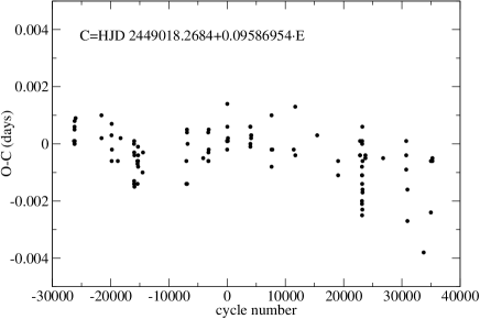
Figure 10: The O$-$C diagram of BE Lyn

The 47 new epochs supplemented the earlier O$-$C diagram, and the final dataset consists of 106 points (references can be found in Kiss & Szatmáry 1995). We plot the resulting O$-$C diagram in Fig. 10. It has been calculated with the following ephemeris:

$$HJD_{\rm max}=2449018.2684+0.09586954\times E$$

(Liu & Jiang 1994). Obviously, the LITE-solution of Kiss & Szatmáry (1995) does not hold, as there is no cyclic feature in the present diagram. Slight variations are suggested but neither a linear nor a parabolic fit describes very well the general appearance.

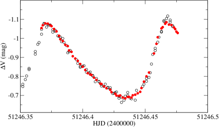
Figure 11: A comparison of two simultaneous datasets of BE Lyn obtained with Sz40 (open circles) and SNO90 (filled circles).

We have made several tests to improve our understanding of the limitations in the case of BE Lyn. First, we have checked the consistency of the determined epochs of maxima with simultaneously obtained observations. On March 8, 1999, there were two cycles observed in parallel with Sz40 and SNO90. We show the light curve comparison in Fig. 11. Spanish data were shifted vertically to the best match with the Hungarian observations. The independent measurements yielded almost the same times of maximum, both were within 0$\aas@@fstack{d}$0002 (see Table 6). So we believe that the estimated accuracy of $\pm$0$\aas@@fstack{d}$0003 for the individual epochs is indeed a realistic value. There is, however, a larger scatter in the O$-$C diagram which appears to be larger than the observational noise. Fourier analysis of the diagram did not help, because both the residuals of the linear fit and the parabolic fit (see below) showed peaks close to the pulsational frequency, implying higher order period change (that is a simple consequence of the curved nature of the diagram) or low-frequency components in the spectrum caused by the inappropriate fit.

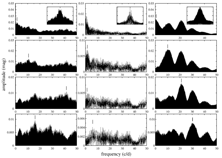
Figure 12: Subsequent Fourier spectra of three subsets (1995-1997, 1999 and 2001) of BE Lyn (three columns) after prewhitening with the dominant frequency and its harmonics. The highest peaks are marked in every spectrum, with which the next prewhitening steps were done, from top to bottom. The small inserts show the window functions. Although there is some evidence for weak secondary periodicity, no features can be identified as being the same in all three subsets. The S/N ratios (Breger et al. 1993) of the marked peaks range from 3 to 10.

Secondly, we have searched low-amplitude secondary periodicity in the light curves. Garrido & Rodríguez (1996) have already tried to detect microvariability of BE Lyn but found nothing, based on five nights of observations obtained with a span of two years. Since we have 27 $V$-band light curves distributed almost uniformly from 1995 to 2002, we performed their Fourier analysis with the same aim. We have divided the data into three subsets, in which the changes of the dominant frequency can be neglected. Nightly mean values have been subtracted (as did, e.g., Kiss et al. 2002a) and that is why we had to exclude a few nights with short light curve coverage from the analysis. The first subset covered 1995-01-31–1997-02-20; the second 1999-01-26–1999-05-14; and the third 2001-02-24–2002-05-01. The most homogeneous and best-quality subset is the second one, which consists mainly of high-precision photoelectric photometry with SNO90.

We prewhitened each subset with $f_{0}=10.430842$ d^-1 and its harmonics up to the fifth order and analysed the residuals for periodicity. The results can be summarized as follows. In every subset, we detected low-frequency ($f<2$ d^-1) components which we attributed to nightly zero-point uncertainties. After their removal, we could not infer any periodicity that was common to all subsets. The prewhitened spectra in Fig. 12 show that, although there are some hints of multiperiodicity, no identical features can be identified in all three subsets. Most importantly, the second subset (middle column in Fig. 12) does not reveal anything with amplitude larger then 5 mmag. Therefore, we conclude that: i) there is no detectable stable secondary periodicity in the light curve of BE Lyn above the mmag level; ii) if the scatter of the O$-$C diagram is real than it implies some light curve instabilities (transient phenomena) which are not strictly periodic but affect the light curve shape. Nevertheless, we admit that the whole effect is just on the limit of detectability and no unambiguous conclusion can be drawn at the present time. And, as noted by Garrido & Rodríguez (1996), the microvariability can be studied only with the highest quality observations (long-term homogeneous photometry with internal precision of a few mmag), which is, unfortunately, not the case for our data.

We have also checked the Fourier amplitude and phase parameters, used to describe the light curve shape, for seasonal variability. We have checked $R_{21}$, $R_{31}$, $\varphi_{21}$ and $\varphi_{31}$ (see, e.g., Poretti 2001) but found no changes. For instance, $R_{21}$ was 0.335, 0.328 and 0.303, while $R_{31}$ varied from 0.108, 0.111, 0.113. As a comparison, the uncertainty of these values is a few in the last digit and we do not consider the mentioned variations as significant. Thus we exclude the presence of long-term light-curve shape changes.

By setting aside the higher-order period change, we have determined an ephemeris correction with a linear fit and estimated the period changing rate with a parabolic fit. The linear approximation yields the following improved ephemeris:

$$HJD_{\rm max}=2449018.2681+0.095869521(4)\times E$$

which can be used to predict forthcoming maxima. The parabolic fit gives $\beta=(-1.3\pm 0.5)\times 10^{-12}$, that would correspond to ${1\over P}{dP\over dt}=(-5\pm 1.9)\times 10^{-8}$ year^-1. However, we consider this value only as an upper limit for the period change, as the present situation is not as clear as for the previous examples. Nevertheless, this limit is in good agreement with theoretical expectations of BP98.

3.6 DY Pegasi

DY Peg is one of the best observed HADSs, with observations dating back more than a half century. A recent update of the period change was published by Blake et al. (2000), while the physical parameters of the star were determined by Wilson et al. (1998) and Peña et al. (1999). Garrido & Rodríguez (1996) presented some evidence for secondary periodicity, although based on only four nights of observations. The most detailed period study is that of Koen (1996), revealing the complex nature of the period variations. Interestingly, even the seemingly simple parabolic O$-$C descriptions yielded ambiguous results: Blake et al. (2000) estimated a quadratic term of the O$-$C diagram almost a factor of seven less than, e.g. Mahdy (1987) ($-1.36\times 10^{-12}$ vs. $-0.231\times 10^{-12}$).

Table 7: Journal of observations and new times of maximum for DY Peg

Date	filter	Inst.	Points	$HJD_{\rm max}$
2001-01-01	$B$	P60	101	2451911.2338
				2451911.3062
2001-08-03	$V$	Sz40	166	2452125.5619
2001-08-04	$V$	Sz40	152	2452126.5833
2001-08-12	$V$	Sz40	253	2452134.5332
				2452134.6062
2001-08-15	$V$	Sz40	339	2452137.5228
				2452137.5955
2001-09-05	$uvby$	SNO90	57	2452158.3805
2001-09-08	$uvby$	SNO90	69	2452161.4431

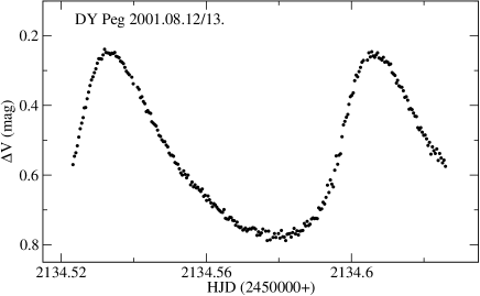
Figure 13: Sample light curve for DY Peg.

Our observations were carried out at three observatories on seven nights in 2001. The full log of observations, supplemented with the new times of maximum, is presented in Table 7. Throughout the observations we used the same comparison star with all of the instruments (HD 218587, $V=9\aas@@fstack{m}80$, $b-y=0\aas@@fstack{m}376$, $m_{1}=0\aas@@fstack{m}180$, $c_{1}=0\aas@@fstack{m}399$, as given in the SIMBAD database). The secondary comparison was either GSC 1712-0542 ($V\approx 11\aas@@fstack{m}7$) or GSC 1712-1246 ($V\approx 11\aas@@fstack{m}1$). The integration time varied between 30 and 120 seconds. A sample light curve is shown in Fig. 13.

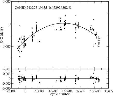
Figure 14: The O$-$C diagram of DY Peg. The solid line denotes the parabolic fit.

After collecting and supplementing the full list of maxima (Blake et al. 2000 and references therein, Van Cauteren & Wils 2000, Agerer et al. 2001) we show in Fig. 14 the final O$-$C diagram covering 1943–2001 with the ephemeris of Mahdy (1987):

$$HJD_{\rm max}=2432751.9655+0.072926302\times E$$

The parabolic fit has to following form:

$$O-C=-0.0037(1)+5.6(2)\times 10^{-8}E-2.0(1)\times 10^{-13}E^{2}$$

with an rms of 0$\aas@@fstack{d}$001. This results in ${1\over P}{dP\over dt}=(-2.79\pm 0.14)\times 10^{-8}$ year^-1, which is in good agreement with Mahdy (1987) and Peña et al. (1987), thus we do not confirm the different result of Blake et al. (2000). We also note that the updated O$-$C diagram is obviously not fully described by the parabolic fit; for instance, the last $\sim 25000$ cycles would need a much steeper function than the present parabola. Therefore, we fully agree with Koen (1996) that viable quantitative alternatives to the traditional O$-$C analysis must be used when investigating the fine details of the period changes. Here we did not go beyond the simplest analysis, because that would lead us too far from the primary purposes of this paper.

3.7 GW Ursae Majoris

The light variations of GW UMa ($\langle V\rangle\approx 9.7$, $A_{\rm V}=0\aas@@fstack{m}44$, $P=0\aas@@fstack{d}2032$) were discovered by the Hipparcos satellite, and despite its brightness and short period, there has been no new observation since the discovery. A special interest can be attributed to this star due to the period value: it is just on the boundary between HADSs and the shortest period RR Lyrae stars (Poretti 2001). In order to place the star in the light curve diagnostic diagrams used by Poretti (2001), we observed the star in $B$, $V$ and $I_{\rm C}$ bands on 6 nights in 2002 (Poretti utilized I-band data of hundreds of stars to infer characteristic Fourier-parameters of HADS and RRc variables). More than 2500 individual points were obtained (the full observing log is presented in Table 8). The comparison star was GSC 3011-2535 ($V\approx 10\aas@@fstack{m}9$).

Table 8: Journal of observations and new times of maximum for GW UMa

Date	filter	Inst.	Points	$HJD_{\rm max}$
2002-04-30	$V$	Sz40	820	2452395.5408
2002-05-01	$V$	Sz40	180	2452396.5584
2002-05-02	$I_{\rm C}$	Sz40	674	2452397.3702
				2452397.5782
2002-05-03	$V$	Sz40	229	2452398.3850:
2002-05-03	$I_{\rm C}$	Sz40	258	2452398.3877
2002-05-22	$B$	Sz40	181	2452417.4858
2002-05-31	$B$	Sz40	204	2452426.4259

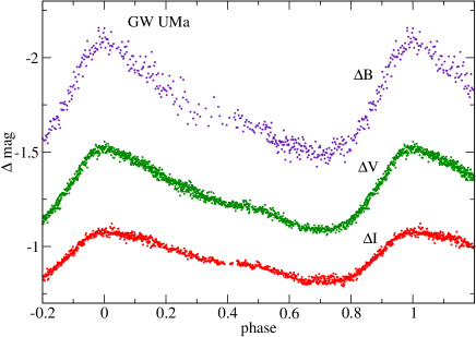
Figure 15: The phase diagrams of GW UMa ($E_{0}$=2452395.5408, $P=0\aas@@fstack{d}2031940$).

Our analysis showed that the star is likely to be monoperiodic, as we could not detect cycle-to-cycle changes of the light curve shape in any band (although this conclusion is based on a fairly scanty dataset). The phased light curves are shown in Fig. 15. The amplitudes in the instrumental $BVI_{\rm C}$ system are 0$\aas@@fstack{m}$62, 0$\aas@@fstack{m}$44 and 0$\aas@@fstack{m}$27, respectively (all but one night of observations were single-filtered, for better time resolution, but the trade-off is the lack of standard transformations). The Fourier amplitude parameter $R_{21}$=0.40 for the $I$-band data placed the star among the HADSs (see Fig. 7 in Poretti 2001). Therefore, we exclude the possibility of first- or second-overtone RR Lyrae pulsation, as suggested for other short-period pulsators of similar light curve shapes and periods (see, e.g. Kiss et al. 1999 for a discussion of the nature of V2109 Cyg which, however, recently turned to be a multiperiodic HADS (Rodríguez, in preparation)). Eight new times of maximum were determined (Table 8) and the mean O$-$C value with the Hipparcos ephemeris ($E_{0}=2448500.1160$, $P=0\aas@@fstack{d}2031940$) is $-0\aas@@fstack{d}0062$ (c.c. $-$9 min), suggesting either inaccurate Hipparcos period, or slight period change during the last decade. Assuming a constant period, we calculated to following corrected ephemeris:

$$HJD_{\rm max}=2448500.1160+0.20319367(3)\times E$$

In any case, further CCD observations are needed to clarify the situation. The star is probably a Pop. II object, as the high galactic latitude ($+59\aas@@fstack{\circ}14$) is associated with large radial velocity (the SIMBAD database lists $-81$ km s^-1). Unfortunately, the Hipparcos parallax is not useful ($0.58\pm 2.88$ mas), thus no other information can be deduced from the presently available data.

4 Summary

In this paper, we presented observational results of an almost 8-year long project, with the main goal of updating our knowledge on the period change of selected bright northern HADSs. Our results strengthen the generally adopted view of evolutionary period changes, and the determined period decreasing and increasing rates are in good accordance with the theory. The most relevant new results are mostly negative results, in the sense of disproving earlier conclusions that appeared in the literature:

1. For DY Herculis, we do not confirm the suspected binarity (Pócs & Szeidl 2000). The updated O$-$C diagram between 1938 and 2001 does not show clear signs of a light-time effect. Instead of that, a quadratic fit is fairly satisfactory.

2. For YZ Bootis, we do not confirm the increase of the period (Hamdy et al. 1986). Instead of that we find slow period decrease, close to the limits of detection.

3. For BE Lyncis, we do not confirm the suspected binarity (Kiss & Szatmáry 1995). The updated O$-$C diagram between 1986 and 2002 suggests complex period variations with no real cyclic nature. Fourier-analysis of the light curves did not reveal possible multiple periodicity above the millimag level. A formal quadratic fit to the O$-$C diagram resulted in an upper limit to the period change rate that is in agreement with the theoretical expectations. Further observations of the star are needed.

4. For DY Peg, we do not confirm the results on its smooth period change rate (Blake et al. 2000). Although there are hints for more complex period variation (see also Koen 1996), the updated O$-$C diagram between 1943 and 2001 can be very well fitted with a parabola that has similar coefficients than in Mahdy (1987) or Peña et al. (1987).

5. We presented the first observations of GW UMa since its discovery by the Hipparcos satellite. Empirical evidence was found for its HADS nature and the available kinematic data suggest the star to be a Pop. II object (thus possibly belonging to SX Phe stars). The period of 0$\aas@@fstack{d}$203 makes the classification an intriguing task, as GW UMa is right on the border between RR Lyrae and HADS stars. The stability of the light curve shape excludes the possibility of a relatively high-amplitude secondary period.

For the remaining two stars (XX Cyg and SZ Lyn), our conclusions are more or less confirmations of previously published results. As expected from the longer time basis available for the target stars, the newly determined quadratic coefficients (and the corresponding period changes) have better defined values and our calculations yielded a slight or significant decrease of the absolute value of the period changes. With these corrections, we find better agreement with theory.

Finally, let us point out again that HADS stars are easy targets for small astronomical instruments. The open questions raised for our programme stars or those of for other bright HADSs make continuous photometric monitoring a useful project for small telescopes under light-polluted urban environment. Even well-equipped amateur astronomers or small colleges can make significant contribution to observational studies of high-amplitude $\delta$ Scuti stars.

- (1) Agerer, F., & Hübscher, J. 2000, IBVS, No. 4912
- (2) Agerer, F., Dahm, M., & Hübscher, J. 1999, IBVS, No. 4712
- (3) Agerer, F., Dahm, M., & Hübscher, J. 2001, IBVS, No. 5017
- (4) Blake, R. M., Khosravani, H., & Delaney, P. A. 2000, JRASC, 94, 124
- (5) Blake, R. M., Delaney, P., Khosravani, H., et al. 2003, PASP, 115, 212
- (6) Breger, M., Stich, J., Garrido, R., et al. 1993, A&A, 271, 482
- (7) Breger, M., & Pamyatnykh, A. A. 1998, A&A, 332, 958
- (8) ESA 1997, The Hipparcos and Tycho Catalogues, ESA SP-1200
- (9) Garrido, R., & Rodríguez, E. 1996, MNRAS, 281, 696
- (10) Hamdy, M. A., Mahdy, H. A., & Soliman, M. A. 1986, IBVS, No. 2963
- (11) Henden, A. A., & Kaitchuk, R. H. 1982, Astronomical Photometry, Van Nostrand Reinhold Company, New York
- (12) Jiang, S. 1985, Acta Astron. Sinica, 26, 297
- (13) Kim, C., & Joner, M. D. 1994, ApSS, 218, 113
- (14) Kiss, L. L., & Szatmáry, K. 1995, IBVS, No. 4166
- (15) Kiss, L. L., & Derekas, A. 2000, IBVS, No. 4950
- (16) Kiss, L. L., Csák, B., Thomson, J., & Vinkó, J. 1999, A&A, 345, 149
- (17) Kiss, L. L., Derekas, A., Alfaro, E. J., et al. 2002a, A&A, 394, 97
- (18) Kiss, L. L., Derekas, A., Mészáros, & Székely, P. 2002b, A&A, 394, 943 (Paper I)
- (19) Koen, C. 1996, MNRAS, 283, 471
- (20) Koen, C., & Lombard, F. 1995, MNRAS, 274, 821
- (21) Liu, Z., & Jiang, S. Y. 1994, IBVS, No. 4077
- (22) Lombard, F. 1998, MNRAS, 294, 657
- (23) Lombard, F., & Koen, C. 1993, MNRAS, 263, 309
- (24) Mahdy, M. A. 1987, IBVS, No. 3055
- (25) Moffett, T. J., Barnes, T. G. III, Fekel, F. Jr., et al. 1988, AJ, 95, 1534
- (26) Paparó, M., Szeidl, B., & Mahdy, H. A. 1988, ApSS, 149, 73
- (27) Peña, J. H., Peniche, R., González, S. F., & Hobart, M. A. 1987, Rev. Mex. Astron. Astrofís., 14, 429
- (28) Peña, J. H., González, D., & Peniche, R. 1999, A&AS, 138, 11
- (29) Peniche, R., González, S. F., & Peña, J. H. 1985, PASP, 97, 1172
- (30) Pócs, M. D., & Szeidl, B. 2000, IBVS, No. 4832
- (31) Pócs, M. D., & Szeidl, B., & Virághalmy, G. 2002, A&A, 393, 555
- (32) Poretti, E. 2001, A&A, 371, 986
- (33) Rodríguez, E. 1999, PASP, 111, 709
- (34) Rodríguez, E., López de Coca, P., Costa, V., & Martín, S. 1995, A&A, 299, 108
- (35) Rodríguez, E., Rolland, A., López de Coca, P., & Martín, S. 1996, A&A, 307, 539
- (36) Szeidl, B., & Mahdy, H. A. 1981, Comm. Konkoly Obs., No. 75
- (37) van Cauteren, P., & Wils, P. 2000, IBVS, No. 4872
- (38) Vinkó, J., Bíró, I. B., Csák, B., et al. 2003, A&A, 397, 115
- (39) Wilson, W. J. F., Milone, E. F., Fry, D. J. I., & van Leeuwen, J. 1998, PASP, 110, 433
- (40) Yang, D., Tang, Q., Jiang, S.-Y., & Wang, H. 1993, IBVS, No. 3831
- (41) Zhou, A.-Y., Jiang, S.-Y., Chayan, B., & Du, B.-T. 2002, ApSS, 281, 699