Detection of Non-Random Galaxy Orientations in X-ray Subclusters of the Coma Cluster

Abstract

This study on the Coma cluster suggests that there are deviations from a completely random galaxy orientation on small scales. Since we found a significant coincidence of hot-gas features identified in the latest X-ray observations of Coma with these local anisotropies, they may indicate regions of recent mutual interaction of member galaxies within subclusters which are currently falling in on the main cluster.

1. INTRODUCTION

Galaxy orientation studies in the past (see Hawley & Peebles, 1975, and references therein) were chiefly carried out in order to verify miscellaneous galaxy cluster formation scenarios. Early theories of cluster formation were the primordial-vorticity, pancake-shock, and tidal-torque theories (for a brief overview see Sugai & Iye, 1995) which had predicted different alignment configurations of cluster members for different birth models respectively. Unfortunately these models were at least incomplete due to the missing knowledge of the presence of dark matter in clusters and the assumption that clusters formed through fragmentation. Putting the focus on finding an orientation pattern for the whole cluster may be the main reason why many investigations in this field did not yield sufficiently unambiguous results (Flin & Godlowski, 1986; Sugai & Iye, 1995; Flin, 2001).

More recent studies concentrated on the orientation of a number of brighter galaxies whose major axis shows a tendency to be aligned along the elongation of the parent cluster (Struble, 1990). For instance the Virgo (West & Blakeslee, 2000) and also the Coma cluster (West, 1997) were found to exhibit this phenomenon which is further discussed in section 5.

Only recently Brown et al. (2002) published their work that tries to give an estimate on the reliability of gravitational lensing studies which assume that anisotropies in the ellipticity distribution are due to a gravitationally induced shear field distorting galaxy images (cf. Tyson et al., 1990), an important aspect briefly picked up in section 5 as well.

In the present work, using extensive data on galaxy position angles and inclinations of a large number of galaxies in Coma (A1656), we are investigating the alignment of the majority of faint cluster members on small scales, even though only in a statistical way. Our method is to perform an individual statistical test for the surroundings of each galaxy in the sample. We show that the found anisotropies are statistically significant to a high extent and superpose an image of average orientations of non-random regions on recent X-ray observations. Since an interesting coincidence emerges this approach seems to be profitable. We also try a tentative interpretation based on current models of galaxy cluster evolution.

2. THE DATA

A huge sample of 6724 galaxies within a region of about $2.6\arcdeg\times 2.6\arcdeg$ centered on Coma was compiled in 1983 by Godwin, Metcalfe, & Peach (GMP hereafter). This is still the most comprehensive catalogue of galaxies in the Coma cluster, comprising galaxies up to a brightness within the $26\fm 5$ contour limit of $b_{26.5}=21\fm 0$. The catalogue is considered complete up to $b_{26.5}=20\fm 0$. Position angle and ellipticity for 4344 entries are included, however no morphological classification is given.

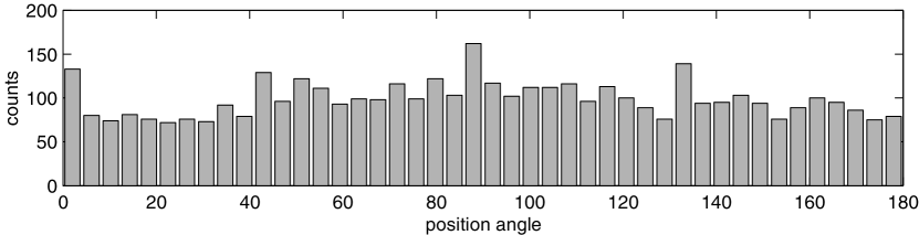
Figure 1.— Distribution histogram of the 4344 position angles in the GMP sample.

The sample as a whole shows a slight overabundance of galaxies with position angles around $90\arcdeg$ (see

Figure 2.— )

with a roughly harmonic shape of period $180\arcdeg$. Also a periodicity of $45\arcdeg$ may be inferred which was presumably caused by the plate scanning process but can be neglected for our purposes since it is smoothed out by the binning process. These global properties have yet been known for quite some time (Djorgovski, 1983). However, a closer look at the respective orientations of the individual galaxies is worthwhile and provides new insights.

3. THE METHOD OF ANALYSIS

Instead of separating the cluster into certain sub-samples which requires us to make assumptions on where we expect to be alignment in the first place, we decided to use the environs of each galaxy as a sub-sample which eliminates such a selection bias.

For each galaxy the angle of intersection between its major axis and the major axes of the 15 closest neighbor galaxies is calculated, whereby 15 was chosen as a reasonable trade-off between small-number statistics and unwanted smoothing of the results. From these differential angles a distribution histogram is created. If the distribution is not in agreement with a random distribution, i.e. it is not isotropic according to a $\chi^{2}$-test, a best fit for the average orientation of this ensemble of adjacent galaxies is derived as described below.

First, the ‘projected spin vector’ $\mbox{\boldmath$P$}_{i}$ of a galaxy with PA $\beta_{i}$ and ellipticities $\epsilon_{i}$ is defined as the vector in the observational plane that is orthogonal to the major axis of the galaxy image and has length $P_{i}=\sin(\eta)$. Here $\eta$ denotes inclination, thus $cos(\eta)=\frac{b}{a}$, $\epsilon=1-\frac{b}{a}$ with axial ratios $\frac{b}{a}$.

$$\mbox{\boldmath$P$}_{i}=P_{i}\left(\cos\beta_{i}\atop\sin\beta_{i}\right)$$ (1)

$$P_{i}^{2}=1-\frac{b^{2}}{a^{2}}=1-(1-\epsilon_{i})^{2}$$ (2)

For the ensemble we define the ‘average projected spin vector’ $S$ with PA $\alpha$

$$\mbox{\boldmath$S$}=S\left(\cos\alpha\atop\sin\alpha\right)$$ (3)

as the vector which satisfies the condition

$$\left\{\sum_{i}(\mbox{\boldmath$S\cdot P$}_{i})^{2}\right\}\longrightarrow\max$$ (4)

The scalar product can be expanded to

$$(\mbox{\boldmath$S\cdot P$}_{i})^{2}=S^{2}P_{i}^{2}\cos^{2}(\alpha-\beta_{i})$$ (5)

Thus $P_{i}^{2}$ can be viewed as the weighting factor of the sum which means that edge-on galaxies have a much stronger weight than (nearly) face-on galaxies for which the PA is more or less arbitrary.

It follows that eq. 4 has the solution:

$$\tan(2\alpha)=\frac{\sum\limits_{i}P_{i}^{2}\sin(2\beta_{i})}{\sum\limits_{i}P_{i}^{2}\cos(2\beta_{i})}=:\frac{S_{y}}{S_{x}}$$ (6)

If we identify x and y in eq. 6 we get the length of vector $S$ by computing $S^{2}=S_{x}^{2}+S_{y}^{2}$

$$S^{2}=\left(\sum_{i}P_{i}^{2}\cos(2\beta_{i})\right)^{2}+\left(\sum_{i}P_{i}^{2}\sin(2\beta_{i})\right)^{2}$$ (7)

4. RESULTS

The map seen in

Figure 3.— s

hows the vector $S$ plotted as black line at the position of each galaxy which is found to possess an anisotropic neighborhood with a level of confidence $\gamma_{\chi^{2}}=0.99$. It is interesting to note that no significant anisotropies are found around the central cD galaxies even though the galaxy density in this region is much higher than anywhere else on the map. Moreover, clearly isolated groups of galaxies with anisotropic orientation can be found.

Even though the algorithm favors such occurrence, the strength of these features is greater than could be expected for a random sample. In order to give an estimate of the statistical significance of our results we performed a series of 1000 runs with artificially generated isotropic data. Apart from being impracticable due to the huge number of runs, a visual assessment of these artificial plots would also be subjective therefore we decided to apply a clustering algorithm to the distribution of $S$. We chose a modified version of K-means clustering which is simple to implement and fast enough for our purpose. The data were clustered in a three-dimensional space spanned by the x and y coordinates of $S$ and as a third coordinate by its PA $\alpha$. The original algorithm had to be modified to be cyclic in $\alpha$. Also we used as a distance measure:

$$r^{2}:=\Delta x^{2}+\Delta y^{2}+C\tan^{2}(\Delta\alpha)$$ (8)

This definition makes sure that two $S$ vectors which have a mutual PA difference of $90\arcdeg$ are infinitely far apart as seen by the clustering algorithm. The scaling factor $C$ can be viewed as weight of $\alpha$. That is to say if $C$ is large the clustering will be very sensitive to small differences in $\alpha$ and vice versa.

The artificial galaxy samples were generated by assigning random PAs to each of the galaxies in the original sample. Moreover the inclinations were shuffled among the sample members which has the advantage of preserving the inclination distribution.

We performed two series of runs with 1000 artificial samples each. The first one included the whole set of 4344 galaxies and a level of confidence for the $\chi^{2}$-test of $\gamma_{\chi^{2}}=0.99$ was chosen while for the second run only those 2354 galaxies brighter than $b_{26.5}\leq 20\fm 0$ were used which made it necessary to decrease $\gamma_{\chi^{2}}$ to a value of 0.97 in order to get enough $S$ vectors to work with (cf. Table 1).

Table 1Definition of the samples

sample	brightness limit	$N$	$\gamma_{\chi^{2}}$
1	$b_{26.5}\leq 21\fm 0$	4344	$0.99$
2	$b_{26.5}\leq 20\fm 0$	2354	$0.97$

The clusters produced by the K-means clustering had to be assessed in an objective way thus we introduced a quality value $q$ for the features found in the artificial samples as well as in the original data:

1. Each feature that contains less than five members (i.e. $S$ vectors) has $q=0$.

2. For each remaining cluster $q$ is defined as the norm of the sum over its constituent $S$ vectors divided by its volume in the three-dimensional cluster space.

Table 2 shows the results obtained for samples 1 and 2. It allows to compare the number $n$ and the quality $q$ of the features in the data to the averaged values for these quantities calculated from the set of artificial samples. Here $q_{A}$ denotes the highest value for $q$ found in the data whereas $\bar{q}_{A}$ is the average of the highest $q$ values calculated from each individual artificial sample.

$$\bar{q}_{A}:=\sum(q_{A}^{i})/1000$$ (9)

Table 2Properties of found anisotropies

	data			artificial			significance
sample	$n$	$q_{A}$		$\bar{n}$	$\bar{q}_{A}$		$\sigma_{n}$	$\sigma_{q}$
1	51	$100000$		29	$16900$		0.997	0.965
2	92	$42900$		71	$10300$		0.957	0.951

The rightmost two columns in Table 2 give the percentage of artificial samples that showed smaller values for $n$ and $q_{A}$ than the data.

$$\sigma_{x}:=\frac{N(x_{i}<x)}{1000}\mbox{~{}~{}~{}with~{}}x\in\{n,q_{A}\}\mbox{,~{}}i\in[1,1000]$$ (10)

It becomes clear that only very few artificially generated samples showed more or better clustered anisotropies than the original data.

Table 3Qualities of top three clusters of a sample

	data			artificial
sample	$q_{A}$	$q_{B}$	$q_{C}$	$\bar{q}_{A}$	$\bar{q}_{B}$	$\bar{q}_{C}$	$\sigma_{q}$
1	$10^{5}$	95800	4490	16854	1054	19	1
2	42900	11000	10300	10340	2391	743	0.999

In order to get a more sophisticated means of assessment we used the three best clusters in a sample denoted $A$, $B$, and $C$ in descending order of quality $q$. For the original data these would be the very strong cluster around NGC4911 ($A$) and the slightly less pronounced ones around NGC4839 ($B,C$). A detailed analysis reveals that clusters $A$ and $B$ comprise 29 distinct galaxies each whereas 39 distinct galaxies cause the anisotropic region around cluster $C$. This can be seen in

Figure 4.— w

hich also shows the spatial distribution of those galaxies.

Table 3 gives the results from comparing the cluster qualities $q_{A},q_{B},q_{C}$ of the three top rated clusters in a sample. Here

$$\sigma_{q}:=\frac{N\left((q_{A}^{i}<q_{A})\wedge(q_{B}^{i}<q_{B})\wedge(q_{C}^{i}<q_{C})\right)}{1000}$$ (11)

and $i$ is the index of the artificial sample as above. None of the artificial samples could produce as many high quality clusters of anisotropically distributed galaxies as the actual data.

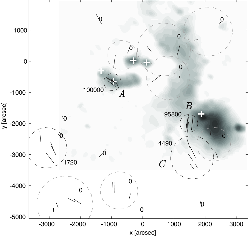
Figure 5.— Map of vectors $S$ for anisotropic galaxy subsamples ($\gamma_{\chi^{2}}$=0.99). Dashed circles denote clusters identified by K-means algorithm, numbers mean quality $q$. The underlying image (extension marked by light grey region) shows X-ray residuals generated by subtracting a $\beta$-model from the Coma cluster X-ray image. White + symbols denote massive galaxies. Origin at $\alpha$=$12^{h}57\fm 3$; $\delta$=$+28\arcdeg 14\farcm 4$ (1950.0), north is up, east is left.

In order to understand their physical meaning it is desirable to verify the visually striking deviations from isotropy in

Figure 6.— b

y comparing them with other measurements of anisotropy in the Coma cluster. An appropriate means to this end can be the underlying image in

Figure 7.— .

It shows the difference between the original X-ray intensity image of Coma and the expected intensity for a so called $\beta$-model, which describes the distribution of hot intra-cluster gas in a completely relaxed cluster. This residual image was recently computed from a mosaic of XMM observations of Coma composed by Neumann et al. (2003) who kindly put their data at our disposal prior to publication. According to them the pronounced feature in the SW around NGC4839 (white + symbol) is a subcluster currently falling on the main cluster. Due to ram pressure inflicted by the intra-cluster gas upon the subcluster, its gas is stripped off and leaves behind a track of hot gas. The same mechanism seems to have produced the slightly less strong residual around galaxies NGC4911 and NGC4921 located SE of the dominating cD galaxy pair in the center.

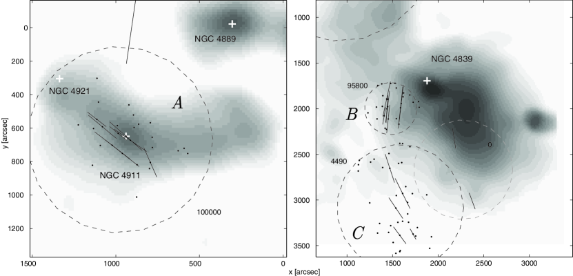
Figure 9.— Enlargements from

Figure 10.— s

howing the best three clusters $A,B,C$ and their surroundings. Black dots denote those galaxies which comprise the neighborhood of the $S$ vectors in the cluster.

In

Figure 11.— i

ndeed a striking coincidence is observed between the regions of statistically significant galaxy alignment and the features emerging in the residual image. Moreover it may also be worth noting that the $S$ vectors around NGC4839 seem to point in a direction tangential to its perimeter while in the case of the NGC4911/NGC4921 pair the anisotropies seem to coincide with the connecting line between the two galaxies.

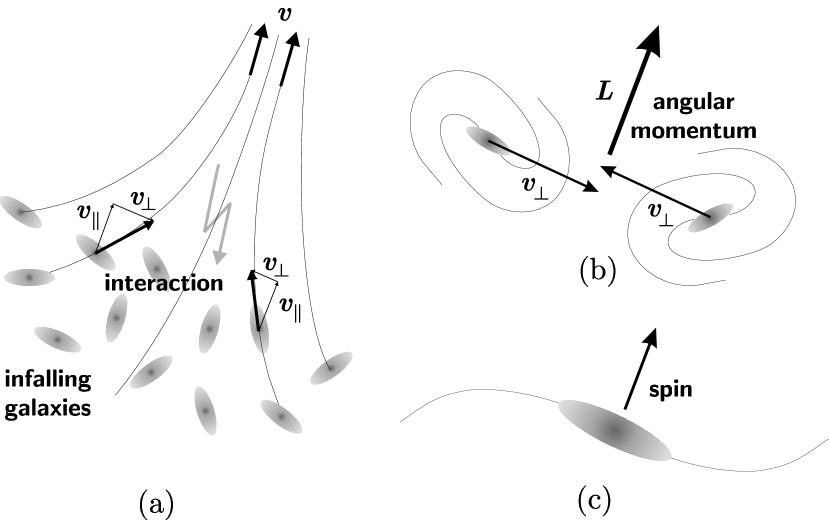
Figure 12.— The Laminar Flow Model: (a) Stream of infalling galaxies – (b) Orbiting galaxies – (c) Merger product

5. INTERPRETATION

A possible explanation for the intriguing match found in

Figure 13.— a

nd

Figure 14.— m

ight be given by a simple model of the dynamical evolution of interacting galaxies falling on Coma along a filament, a process seemingly very common for galaxy clusters (Plionis & Basilakos, 2002; Kim et al., 2002; Novikov et al., 1999). What we called the Laminar Flow Model (LFM) is outlined in

Figure 15.— .

1. Galaxies are streaming into the main cluster from outside. The velocity vectors of two neighboring galaxies can be decomposed into components parallel ($\mbox{\boldmath$v$}_{\parallel}$) and perpendicular ($\mbox{\boldmath$v$}_{\perp}$) to the velocity vector $v$ of the center of mass (CoM).

2. If viewed in a co-moving reference frame with origin in the CoM, the two galaxies orbit each other prior to merging. Their angular momentum vector $\mbox{\boldmath$L$}\sim\mbox{\boldmath$r\times v$}_{\perp}$ lies in a plane orthogonal to $\mbox{\boldmath$v$}_{\perp}$ by definition. Thus the projection of $L$ upon the observational plane is statistically more likely to be aligned parallel to the infall direction $v$.

3. Finally, after the merging has taken place, the resulting galaxy tends to possess a spin vector parallel to the previous angular momentum $L$.

Basically the process can be viewed as funneling of galaxies along the filaments. Perpendicular to the infall direction matter is coalescing and getting denser whereas parallel to its motion vector $v$ it is stretched due to tidal forces. Thus the probability for a merger is higher if the component of the radius vector $r$ parallel to $v$ is small. From the definition of $L$ and

Figure 16.— (

b) it follows that the observed spin alignment can be explained by the LFM. Moreover it is in accordance with the view favored by Maller & Dekel (2002) which holds that the spin vector of galaxies is chiefly determined by the last few merging events.

The ostensible contradiction with the findings of, for instance, West & Blakeslee (2000) that the major axes of the brightest cluster galaxies are aligned with the filaments, can be resolved by considering the different mechanism that produces the bright central cD galaxies. They are the final destination of the infalling matter whose linear momentum is thus converted into angular momentum by the ultimate merger with one of those cosmic cannibals.

Finally the issue of weak lensing should not remain unmentioned. On one hand a detected orientation anisotropy in a sample of galaxies may be caused by gravitational lensing, on the other hand if the anisotropies are real they may give wrong lensing indications if not allowed for. These considerations are beyond the scope of this paper but further investigation may be worthwhile.

6. CONCLUSION

In this work we find that the overall isotropic appearance of galaxy orientations in Coma can not be maintained when looking at galaxy ensembles on the smaller scales of subclusters. These fluctuations are not caused by statistical variations but there exists strong evidence that they are the result of anisotropic merging of subcluster members which fall on the main cluster presumably along filaments extending between large clusters. Therefore the identification of regions in which galaxies show statistically significant deviations of their spin vectors from isotropy may help to trace such filaments as well as provide a new and useful tool to investigate the evolution of galaxy clusters.
Acknowledgments: The mosaic of X-ray observations of the Coma cluster was provided by courtesy of D. Neumann (cf. Neumann et al., 2003).

References

- Brown et al. (2002) Brown, M. L., Taylor, A. N., Hambly, N. C., & Dye, S. 2002, MNRAS, 333, 501
- Djorgovski (1983) Djorgovski, S. 1983, ApJ, 274, L7
- Flin (2001) Flin, P. 2001, MNRAS, 325, 49
- Flin & Godlowski (1986) Flin, P., & Godlowski, W. 1986, MNRAS, 222, 525
- Godwin et al. (1983) Godwin, J. G., Metcalfe, N., & Peach, J. V. 1983, MNRAS, 202, 113
- Hawley & Peebles (1975) Hawley, D. L., & Peebles, P. J. E. 1975, AJ, 80, 477
- Kim et al. (2002) Kim, R. S. J., Annis, J., Strauss, M. A., & Lupton, R. H. 2002, in ASP Conf. Ser. 268: Tracing Cosmic Evolution with Galaxy Clusters, 395
- Maller & Dekel (2002) Maller, A. H., & Dekel, A. 2002, MNRAS, 335, 487
- Neumann et al. (2003) Neumann, D. M., Lumb, D. H., Pratt, G. W., & Briel, U. G. 2003, A&A, 400, 811
- Novikov et al. (1999) Novikov, D. I., Melott, A. L., Wilhite, B. C., Kaufman, M., Burns, J. O., Miller, C. J., & Batuski, D. J. 1999, MNRAS, 304, L5
- Plionis & Basilakos (2002) Plionis, M., & Basilakos, S. 2002, MNRAS, 329, L47
- Struble (1990) Struble, M. F. 1990, AJ, 99, 743
- Sugai & Iye (1995) Sugai, H., & Iye, M. 1995, MNRAS, 276, 327
- Tyson et al. (1990) Tyson, J. A., Wenk, R. A., & Valdes, F. 1990, ApJ, 349, L1
- West (1997) West, M. J. 1997, in eprint arXiv:astro-ph/9709289, 9289
- West & Blakeslee (2000) West, M. J., & Blakeslee, J. P. 2000, ApJ, 543, L27