Planet Migration and Binary Companions: the case of HD $80606$b

Abstract

The exo-solar planet HD $80606b$ has a highly eccentric ($e=0.93$) and tight ($a=0.47$ AU) orbit. We study how it might arrive at such an orbit and how it has avoided being tidally circularized until now. The presence of a stellar companion to the host star suggests the possibility that the Kozai mechanism and tidal dissipation combined to draw the planet inward well after it formed: Kozai oscillations produce periods of extreme eccentricity in the planet orbit, and the tidal dissipation that occurs during these periods of small pericentre distances leads to gradual orbital decay. We call this migration mechanism the ’Kozai migration’. It requires that the initial planet orbit is highly inclined relative to the binary orbit. For a companion at $1000$ AU and an initial planet orbit at $5$ AU, the minimum relative inclination required is $\sim 85\deg$. We discuss the efficiency of tidal dissipation inferred from the observations of exo-planets. Moreover, we investigate possible explanations for the velocity residual (after the motion induced by the planet is removed) observed on the host star: a second planet in the system is excluded over a large extent of semi-major axis space if Kozai migration is to work, and the tide raised on the star by HD $80606$b is likely too small in amplitude. Lastly, we discuss the relevance of Kozai migration for other planetary systems.

1. INTRODUCTION

Ongoing radial-velocity surveys have uncovered $\sim 100$ exo-solar giant planets. Their orbital characteristics are puzzling: many have eccentricities much higher than the planetary orbits in our solar system, and a large fraction reside very close to the host star. These orbits indicate either a formation scenario different from that which operated in our solar system, or a migration mechanism to bring the planets in from large distances.

The object HD $80606$b (Naef, Latham & Mayor et al. , naef (2001), hereafter NLM, period $111.8$ days, $m_{p}\sin i=3.4M_{J}$) the focus of this article, has the highest eccentricity ($e=0.927\pm 0.012$) and the smallest pericentre distance ($\sim 7R_{\odot}$) among all known exo-planet candidates. Is it possible to form such a system in-situ? Among the spectroscopic binaries contained in the Batten catalog (Batten, Fletcher & MacCarthy batten (1989)), the only G-type binary that has a comparably small periastron distance ($\sim 6R_{\odot}$) is HD 27935 (Griffin, Griffin & Gunn et al. , griffin (1985)) with $e=0.85$. Duquennoy, Mayor & Andersen et al. (Gl586 (1992)) reported a more eccentric system, the K-dwarf binary Gl 586A, with $e=0.975$ and a periastron distance of $10R_{\odot}$. However, doubts exist as to whether the latter binary can be primordial. But assuming both systems are primordial, their presence empirically suggests that HD $80606$b might have formed as a binary companion to HD $80606$. This hypothesis is currently untestable, the more so since the projected mass-ratio in this system is rather extreme. Instead we ask the following question: can HD $80606$b be formed in the cool outer part of a protoplanetary disk and then evolve into the current orbit via migration?

Planet-planet scattering is one such possibility, assuming HD $80606$ had or has multiple planets. Ford, Havlikova & Rasio (ford (2001)) integrated the evolution of $\sim 10^{3}$ two-planet systems that are initially dynamically unstable. Not a single close encounter produces a planet with $e>0.90$. This rarity leads us to conclude that either the orbits of most observed exo-planets are results of planet-planet scattering, or that the HD $80606$ system is not the result of such scattering.

The leading hypothesis for planet migration involves gravitational interactions between the planets and the gas disks out of which they form (Goldreich & Tremaine gt (1980); Lin, Bodenheimer & Richardson lbr (1996)). Under certain circumstances planet-disk interactions may also excite the orbital eccentricity of the planet (see, e.g., Goldreich & Sari goldsari (2002)). If so, this may explain the orbital separation and eccentricity of the bulk of the systems discovered so far. These systems exhibit an eccentricity distribution that is roughly flat below $e\sim 0.6$ and distinctly drops off around $0.6$. It is believed that Jupiter-mass planets can open up gaps in their natal gas disks with a fractional width $\Delta a/a$ reaching up to a similar value. This coincidence suggests that passage of an eccentric planet through the disk on either side of the gap tends to damp the planet’s orbital eccentricity and to limit the maximum eccentricity planet-disk interaction produces to $e\sim 0.6$. However, HD $80606b$ stands out with $e=0.93$.

The origin of the orbit of HD $80606$b becomes more perplexing if we consider tidal effects. Assuming that the planet has a tidal dissipation efficiency similar to other known exo-planets (quality factor $Q_{p}=3\times 10^{5}$, Wu wu (2002)) or to Jupiter (Goldreich & Soter goldreich (1966), Peale & Greenberg peale (1980)) and setting its true mass equal to the minimum mass, its radius to a Jupiter radius, we find that a mere $650$ Myrs ago, HD $80606$b had an implausibly high eccentricity of $e=0.99$. The age of the system is likely to be this old or older; the stellar projected rotational velocity is low, $v\sin i\approx 0.9\,\rm km/\,\rm s$, typical of old G-dwarves; it is also chromospherically quiet.

Interestingly, there is a neighbor to this system, HD $80607$, a main-sequence companion $\sim 1000$ AU away. This prompts us to develop a theory in which the companion is responsible for the high eccentricity and small orbit of the planet. There are two ingredients in our theory. First, we assume that the planet was born on an orbit of a few AU, and had an orbital plane inclined relative to the stellar binary plane. The remote stellar companion would induce an eccentricity oscillation in the planet’s orbit via the Kozai mechanism (Kozaikozai (1962); see also discussions by Holman, Touma & Tremaine holman (1997), Innanen, Zheng, & Mikkola et al. , innanen (1997), and Mazeh, Krymolowski & Rosenfeld mazeh (1997)). The second component is tidal circularization. The tides operate most effectively during episodes of high eccentricity in the Kozai cycle. We rely on the dissipative tidal process to irreversibly draw the planet inward. Combining the two processes, we can explain the current high eccentricity as well as the tight orbit. We refer to this planet migration scenario as ‘Kozai migration’.

Eggleton, Kiseleva & Hut (EKH (1998)), Kiseleva, Eggleton & Mikola (kem (1998)), and Eggleton & Kiseleva-Eggleton (EKE (2001), EKE hereafter), have developed this scenario to explain some hierarchical triple star systems. Blaes, Lee & Socrates (omer (2002)) applied an analogous scheme (gravitational radiation being the dissipation mechanism) to hierarchical triple black holes in galactic centers. In this article, we adopt the formalism of EKE in an attempt to produce a plausible life-history for HD $80606$b (§2). The story depends on the value of the tidal quality factor $Q$ (§3.1). The observational consequences of such a life-history follow in §3.2. In §3.3 we discuss the tidal velocities induced at the stellar photosphere by the highly eccentric planet, and the possibility of observing such tides. NLM note the presence of substantial residuals to the Keplerian fit in the HD $80606$ system. The tidal velocities appear to be large, but not large enough to explain the observed velocity residuals. Lastly (§3.4), we assess the importance of Kozai migration for other planetary systems where binary companions are also known to exist.

2. Kozai Migration for HD $80606$b

The host star of HD $80606$b is known to be a member of a common proper-motion binary with a companion (HD $80607$) that is similar to HD $80606$ in both spectral type and metallicity . The two stars are separated by $\sim 20^{\prime\prime}$ on the sky. Unfortunately, it is hard to translate this into a linear dimension. The Hipparcos distances for both stars are highly uncertain This complicates an age determination with isochrone fitting. But if we enforce the constraint that the stars have reached the main-sequence, isochrone fitting yields a lower limit of $\sim 65$ pc on the distance, implying a projected binary separation of $1300$ AU at the current epoch. On the other extreme, requiring that the stars have not yet ascended the red giant branch yields a maximum distance of $\sim 125$ pc, and a projected separation of $2500$ AU. As noted above, the low $v\sin i$ and the chromospheric quietness of HD $80606$ are typical of an old G-dwarf. In this article, we adopt a value of $1000$ AU for the binary semi-major axis ($a_{c}$). The eccentricity is taken to be $e_{c}=0.5$. We discuss the effects on the Kozai migration when $a_{c}$ is increased.

Even at such a large distance, the companion star could significantly perturb the planet orbit as long as the two orbital planes are initially inclined to each other more than $39.2\deg$. Secular effects of the Kozai type could then occur and produce large cyclic variations in the planet’s eccentricity ($e_{p}$) and relative inclination, as a result of angular momentum exchange with the companion orbit. Effects on the companion orbit produced by the planet can be neglected, given the extreme ratio in the two orbits’ angular momenta ($a_{c}\gg a_{p}$ and $m_{c}\gg m_{p}$). Under this approximation, the z-component of the planet’s angular momentum, $J_{z}=\sqrt{GM_{\star}a_{p}}M_{p}\sqrt{1-e_{p}^{2}}\cos I$, is conserved. Here the z-axis is normal to the companion plane. As $a_{p}$ is not modified by secular perturbations, the Kozai integral $H_{K}=\sqrt{1-e_{p}^{2}}\cos I$ is conserved during the oscillations. Minima in $e_{p}$ concur with maxima in $I$, and vice versa. Each Kozai cycle lasts a time $\sim P_{c}^{2}/P_{p}$, or a few Myrs.

A much slower process, tidal circularization, gradually removes energy from the orbit and draws the planet inward. An initially more highly inclined orbit (larger $I$) could reach higher eccentricity. And since the dissipation process depends sensitively on the nearest approach distance between HD $80606$b and its host star, such an orbit would suffer stronger orbital decay and have shorter migration timescale. The key issue in Kozai migration is therefore the initial value of $I$. In §2.1, we first estimate the minimum initial inclination required for migrating HD $80606$b from an initial orbit of $a_{p}=5$ AU and an initial eccentricity of $e_{p}=0.1$, we then confirm this estimate numerically in §2.2.

Symbol	Definition	Fiducial Values
$M_{\star},M_{c},M_{p}$	stellar (host & companion) and planetary masses	$1.1M_{\odot}$, $1.1M_{\odot}$, $7.80M_{J}$
$R_{\star},R_{p}$	stellar and planetary radii	$R_{\odot}$, $R_{J}$
$k_{2\star},k_{2p}$	tidal Love number	$0.028$, $0.51$
$r_{g\star},r_{gp}$	gyro-radius, moment of inertia $=r_{g}MR^{2}$	$0.08$, $0.25$
$Q_{\star},Q_{p}$	tidal dissipation quality factors	$10^{6}$, $3\times 10^{5}$
$\Omega_{\star},\Omega_{p}$	spin frequency	initially $20$ days & $10$ hours
$a_{p}$, $e_{p}$, $n_{p}$ & $P_{p}$	planet semi-major axis, eccentricity, mean motion & period	$n_{p}=\sqrt{G(M_{\star}+M_{p})/a_{p}^{3}}$
$a_{c}$, $e_{c}$, $n_{c}$ & $P_{c}$	parameters for the companion orbit	$a_{c}=1000$ AU, $e_{c}=0.5$

2.1. Minimum Initial Inclination: heuristic argument

To estimate the minimum initial inclination, we note that while the Kozai oscillation roughly conserves $\sqrt{(}1-e_{p}^{2})\cos I$ and $a_{p}$ during individual cycles, tidal circularization preserves orbital angular momentum ($J=\sqrt{GM_{\star}}M_{p}\sqrt{a_{p}(1-e_{p}^{2})}$) during episodes of maximum eccentricity. The planetary spin is quickly (pseudo-)synchronized with the orbital motion, while the star’s synchronization time greatly exceeds the orbital circularization time. Hence the planet’s orbital angular momentum cannot be absorbed into spin. Since $e_{p}\sim 1$ near maximum, conservation of $J$ translates into a constant periastron distance between maximum $e_{p}$ during the Kozai cycles.

In an orbit with a semi-major axis of $5$ AU, HD $80606$b would have to reach an eccentricity as high as $0.993$ (at some point during the Kozai cycle) in order to produce the currently observed periastron. Adopting a minimum of $I\approx 40\deg$ during the Kozai cycles (see, e.g., Holman et al. , holman (1997)), the Kozai integral ( $\sqrt{(}1-e_{p}^{2})\cos I$) remaining constant yields $I\geq 84.8\deg$ for an initial $e_{p}=0.1$. In other words, the two orbits had to be virtually perpendicular to each other when the planet formed. This conclusion is independent of the companion orbital separation.

The planet in HD $80606$b is not currently undergoing Kozai oscillations; the Kozai mechanism operated only when the planet had a semi-major axis $a\geq 4$ AU. To see why, note that the torque exerted by the companion star on the planet has its value and direction dependent on the pericentre argument of the planet ($\omega_{p}$). If, however, this argument also precesses under other forces, the averaged Kozai torque is reduced. General relativistic effects, tidal effects, and rotational quadrapolar bulges on the planet are mainly responsible for these extra precession. Their rates are summarized here (Sterne sterne (1939), Einstein einstein (1916)), with definitions for the symbols listed in Table 1.,

$$\hskip-14.22636pt{d\omega_{p}\over dt}\Bigr{|}_{\rm GR} = 3n_{p}\,{{GM_{\star}}\over{a_{p}c^{2}(1-e_{p}^{2})}},$$ (1a)

$$\hskip-19.91684pt{d\omega_{p}\over dt}\Bigr{|}_{\rm rot}\,\, = {1\over 2}n_{p}{k_{2}\over{(1-e_{p}^{2})^{2}}}\!\left({{\Omega_{p}}\over{n_{p}}}\right)^{2}\!\!{{M_{\star}}\over{M_{p}}}\!\!\left({{R_{p}}\over{a_{p}}}\right)^{5},$$ (1b)

$$\hskip-19.91684pt{d\omega_{p}\over dt}\Bigr{|}_{\rm tide} = {15\over 2}n_{p}k_{2}\!{{1+\frac{3}{2}e_{p}^{2}+\frac{1}{8}e_{p}^{4}}\over{(1-e_{p}^{2})^{5}}}{{M_{\star}}\over{M_{p}}}\!\!\left({{R_{p}}\over{a_{p}}}\right)^{5}.$$ (1c)

Taking a Kozai precession rate of $\sim 0.5n_{c}^{2}/n_{p}/(1-e_{c}^{2})^{3/2}$ (Holman et al. , holman (1997)), and assuming that the planet is pseudo-synchronously spinning with the orbit ($e_{p}=0.1$), the relative precession rates are,

$${{\dot{\omega}_{p}|_{\rm GR}}\over{\dot{\omega}_{p}|_{\rm Kozai}}} \approx 5900\left({{a_{1}}\over{0.47{\rm AU}}}\right)^{-4}\!\!\left({{a_{c}}\over{1000{\rm AU}}}\right)^{3},$$

$${{\dot{\omega}_{p}|_{\rm rot}}\over{\dot{\omega}_{p}|_{\rm Kozai}}} \approx 750\left({{a_{1}}\over{0.47{\rm AU}}}\right)^{-8}\!\!\left({{a_{c}}\over{1000{\rm AU}}}\right)^{3}\!\!\left({{R_{p}}\over{R_{J}}}\right)^{5},$$

$${{\dot{\omega}_{p}|_{\rm tide}}\over{\dot{\omega}_{p}|_{\rm Kozai}}} \approx 270\left({{a_{1}}\over{0.47{\rm AU}}}\right)^{-8}\!\!\left({{a_{c}}\over{1000{\rm AU}}}\right)^{3}\!\!\left({{R_{p}}\over{R_{J}}}\right)^{5}\!\!\!\!.$$ (2)

If any of the above ratios exceeds unity, the Kozai oscillation is destroyed. Setting the first ratio to unity, we obtain a suppression radius $\approx 4$ AU. Currently, the Kozai oscillations are strongly suppressed by these extra precessions. This conclusion does not affect the minimum inclination required for Kozai migration. However, the suppression radius does depend on the companion separation: e.g., it is reduced to $\approx 1.5$AU if the companion semi-major axis is as small as $250$ AU.

2.2. Numerical Integration

We adopt the set of equations (eq. [11]-[17]) in EKE (also see Eggleton, Kiseleva & Hut EKH (1998)) to describe the secular evolution of the planet orbit, as well as the spin of the host star and the planet. Any change in the companion’s orbit is ignored. Physical effects described by these equations include: secular interactions, GR, tidal and rotational precession, and tidal dissipation. These equations are explicitly listed in Appendix A.

We integrate equations (A1)-(A7) starting from the following initial conditions: planet orbit $a_{p}=5.0$ AU, $e_{p}=0.1$, relative inclination $I=85.6\deg$ (slightly higher than the $84.8\deg$ estimate in §2.1 because the actual minimum inclination is $\sim 48\deg$, not $\sim 40\deg$ as we assumed), and periapse angle $\omega_{p}=45\deg$.

Values of the system parameters are listed in Table 1. The resulting orbital and spin information are presented in Fig. 1 as functions of time. Initially, the planet undergoes Kozai oscillation with each cycle lasting $\sim 20$ Myrs. Whenever $e_{p}$ evolves close to maximum, a small amount of energy (but not angular momentum) is removed from the orbit. Both $a_{p}$ and $e_{p}$ are decreased, while $a_{p}(1-e_{p})$ remains roughly constant. This corresponds to a small kick to reduce $e_{p}$ whenever $\omega_{p}\approx\pi/2$ (see Fig. 3 of Holman et al. holman (1997)). The Kozai integral slowly increases. This explains why the amplitude of $e_{p}$ oscillation shrink as the planet migrates inward (top-left panel of Fig. 1). After about $0.7$ Gyrs, the planet has reached an orbit with $a_{p}\sim 2.5$ AU, and the Kozai oscillation is completely destroyed by GR precession. At this epoch, we find $e_{p}\sim 0.99$ and $I\sim 50\deg$. From this point on, tidal circularization dominates the evolution, and the influence of the binary companion is negligible. The planet reaches an orbit of $e_{p}=0.927$ and $a_{p}=0.47$ AU $\sim 1.2$ Gyrs after its birth.

A few notes are in order.

We adopt a value of $Q_{p}=3\times 10^{5}$ for the planet, and $Q_{\star}=10^{6}$ for the host star. We discuss the reasons for these choices in §3.1. Using them, the planet’s spin reaches synchronicity with the orbital frequency near periastron almost instantly, while the star’s spin is hardly affected by tides (see lower-right plot of Fig. 1). Tidal circularization is dominated by dissipation in the planet over that in the star by a factor of $\sim 10$. Most of the dissipation, which conserves orbital angular momentum, occurs when the planet has been driven to maximum eccentricity by the companion star.

The results do not depend on the value for the longitude of the ascending node. This is because in the quadrapole approximation for secular interactions, the companion orbit is effectively taken to be circular so there is no preferred axis in the binary plane. This also explains why the vertical angular momentum of the planet orbit (Kozai integral) is conserved – there is a rotational invariance with respect to the $z$ axis.

The results also do not depend on the value for the argument of pericentre, $\omega_{p}$. Kozai oscillations can cause either circulation or libration in the value of $\omega_{p}$. Fig. 3 of Holman et al. (holman (1997)) shows that the circulating solutions can reach higher $e_{p}$ and therefore should lead to shorter evolutionary timescale. However, for the initial conditions we adopted, the circulating and librating solutions essentially coincide and give rise to similar values for the maximum eccentricity.

To migrate the planet from a distance larger than $5$AU, one requires a higher minimum inclination so as to reach the same pericentre distance at maximum eccentricity. In comparison, this inclination hardly varies when the initial eccentricity of the planet is varied from $0.1$ to $0.6$, this can be seen from Fig. 1. Lastly, if the companion is further away than $1000$ AU, each Kozai cycle lasts longer, and it takes a longer time for the planet to migrate to its current location. For instance, placing the companion at $a_{c}=1500$ AU, we find the planet should now be $\sim 5$Gyrs old.

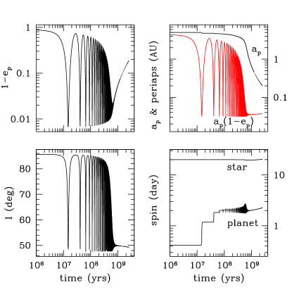
Figure 1.— Evolution of the planetary orbit as a function of logarithmic time (in years). The four panels represent (from left to right, up to down), evolution of the planet eccentricity, planet semi-major axis and periastron distance (in AU), inclination of the planet plane relative to the stellar binary plane, and spin periods for both the planet and the star (in days). See the text for the choice of parameters. During the Kozai cycles, maxima in eccentricity concur with minima in inclination. At the current orbit ($e_{p}=0.927$ and $a_{p}=0.47$ AU), the planet no longer undergoes Kozai oscillations as a result of GR and tidal precession. The dashed part of each curve depicts future evolution of the planet orbit under tidal circularization.

3. Discussion

3.1. $Q$ Value

A time-dependent tide raised on a celestial body, due to either its asynchronous rotation (asynchronous tide) or its eccentric movement (eccentricity tide), can be dissipated, leading to synchronous spin or orbital circularization. The rate of dissipation is conventionally described by a dimensionless quality factor $Q$, the ratio between the energy in the tidal bulge and the energy dissipated per orbital period. For equilibrium tides, $Q$ is related to the lag-angle between the tide-inducing object and the tidal bulge $\delta$ by $\delta\approx 1/2Q$.

It is possible to adapt the $Q$ description to dynamical tides, in which case the tidal energy refers to the energy in the (non-existent) equilibrium tidal bulge, and $Q$ is obtained from the dissipation averaged over a range of tidal frequencies. Back-reaction to the orbits by the gravitational moments of the tidal waves is ignored, a procedure strictly justifiable only when the damping time of the waves is shorter than the orbital period. However, secular effects of the tidal dissipation should be independent of this back-reaction.

Jupiter’s $Q$ value has been estimated to be $10^{5}\lesssim Q\lesssim 2\times 10^{6}$, with the actual value believed to be closer to the lower limit (Goldreich & Soter goldreich (1966), Peale & Greenberg peale (1980)), based on the resonant configuration of the Galilean satellites. The physical origin of this $Q$ value has remained elusive for a few decades. As is explicitly shown in Wu (wu (2002)), exo-planets share similar $Q$ values ($Q_{p}\sim 3\times 10^{5}$) as Jupiter. This is striking as the exo-solar planets have different thermal environments, formation histories, and possibly interior compositions, than those of Jupiter. The similar $Q$ values provide an important clue as to the underlying dissipation mechanism. Moreover, while the $Q$ factor for Jupiter pertains to the asynchronous tide, the one for exo-planets concerns the eccentricity tide. One may speculate that the quality factors for the different Jovian-mass objects agree because all the objects rotate fast with periods comparable to or shorter than the tidal period.

Tidal dissipation in the host star of HD $80606$b also contributes to circularization. What is the tidal $Q$ factor appropriate for solar-type stars? Field solar-type binaries are observed to be circularized out to $\sim 12$ day orbits (Duquennoy & Mayor duqu (1991)). This would imply $Q\sim 10^{5}$ adopting an age of $5$ Gyrs. These binary stars have presumably been synchronized, so this $Q$ value is affiliated with dissipation of the eccentricity tide in rapidly spinning objects ($Q_{\rm fast}$). For the evolution of planet orbits, the $Q$ value of relevance is that for the asynchronous tide in slowly rotating objects to which most host stars belong ($Q_{\rm slow}$). It is not clear that $Q_{\rm fast}$ is directly related to $Q_{\rm slow}$. What observational constraints could we put on $Q_{\rm slow}$?

Short period planets can tidally spin up the star, at the cost of planetary orbital decay. Assuming all host stars are Sun-like and all exo-planets are Jupiter-like, we obtain a lower limit of $Q_{\rm slow}>10^{5}$ if all planets are to survive in their current orbit for another $5$ Gyrs.

Drake et al. (drake (1998)) considered the rotational velocities for three planet-bearing stars ($\tau$-Boo, $\upsilon$-And, and 51 Peg). Among them, $\tau$-Boo has the closest and most massive planet and appears to be synchronized, while the other two have not. Taken at face value, this would imply $Q_{\rm slow}\approx 10^{4}$. This contradicts our earlier statement that $Q_{\rm slow}>10^{5}$. These two results can be reconciled either by the imminent death of the shortest period planets, or by the possibility that $\tau$-Boo has had only its surface convective layer synchronized with the orbit (see Goldreich & Nicholson goldreich2 (1989) for a similar argument on massive stars). The latter possibility also makes it difficult to infer $Q_{\rm slow}$ using the spin data of solar-type binaries. It is interesting to notice that among the three stars discussed by Drake et al. (drake (1998)), $\tau$-Boo likely has the thinnest convective envelope.

Unable to infer hard constraints on $Q_{\rm slow}$, we decide to adopt $Q_{\star}=Q_{\rm slow}=10^{6}$ in our study. With this choice, dissipation in the planet is roughly $10$ times more important than dissipation in the star even for a planet as massive as $M_{p}=7.8M_{J}$. This choice has the advantage that unless the actual $Q_{\star}$ is much lower, the results presented here are not qualitatively affected.

3.2. Constraints on possible Second Planets

If there existed a second planet in the system, secular interaction between this planet and HD $80606$b may destroy the Kozai oscillations. Kozai oscillations require that the precession caused by a second planet acting on HD $80606$b’s orbit be no larger than that produced by the companion star (Innanen et al. , innanen (1997)). We briefly investigate what constraints this puts on the mass and orbit of the second planet.

We assume the two planets have coplanar orbits and the second planet (denoted with subscript $s$) lies inward of the orbit of HD $80606$b. The derivation is similar if it lies outward. Secular interaction between the two planets alone gives rise to variations in their eccentricities ($e$) and periapse angles ($\omega$). Adopting a complex variable $I=e\,\exp(i\omega t)$, and assuming that $e\ll 1$, the first-order secular evolution equations read (Murray & Dermott MD2000 (2000), hereafter MD2000),

$${{dI_{s}}\over{dt}}=iA_{ss}I_{s}+iA_{sp}I_{p},\hskip 5.69046pt{{dI_{p}}\over{dt}}=iA_{ps}I_{s}+iA_{pp}I_{p},$$ (3)

where the real coefficients $A_{ij}$ are

$$A_{ss} = {{\alpha^{2}}\over{4}}{{M_{p}}\over{M_{\star}}}n_{s}B_{1},\hskip 5.69046ptA_{sp}=-{{\alpha^{2}}\over{4}}{{M_{p}}\over{M_{\star}}}n_{s}B_{2},$$

$$A_{ps} = -{{\alpha}\over{4}}{{M_{s}}\over{M_{\star}}}n_{p}B_{2},\hskip 23.9002ptA_{pp}={{\alpha}\over{4}}{{M_{s}}\over{M_{\star}}}n_{p}B_{1}.$$ (4)

Here, $n_{s}=\sqrt{G(M_{\star}+M_{s})/a_{s}^{3}}$, $\alpha=a_{s}/a_{p}$, and $B_{1}=b_{3/2}^{(1)}(\alpha)$, $B_{2}=b_{3/2}^{(2)}(\alpha)$ with $b_{i}^{(j)}$ being the usual Laplace coefficients (MD2000). The general solution to eq. (3) is composed of two linear eigenvectors with their respective precession rates

$$g_{\pm}={{(A_{ss}+A_{pp})\pm\sqrt{(A_{ss}-A_{pp})^{2}+4A_{sp}A_{ps}}}\over 2}.$$ (5)

We are able to approximate the precession rate of HD $80606$b under secular interaction as,

$${{d\omega_{p}}\over{dt}}\Bigr{|}_{\rm sec} = {\rm Min}(g_{+},g_{-})\hskip 14.22636pt{\rm{if\,\,M_{p}>M_{s}}},$$ (6)

$${\rm Max}(g_{+},g_{-})\hskip 14.22636pt{\rm{if\,\,M_{p}<M_{s}}}.$$

At birth, HD $80606$b could not have undergone Kozai oscillation if the second planet is massive enough. Requiring the above secular precession rate to be smaller than the Kozai precession rate (see eq. [2]) when $a_{p}=5$ AU, we find that the mass of the second planet is constrained to a value that depends on its distance to HD $80606$b. This is depicted in Fig. 2.

These results also strongly constrain the current state of the planetary system. No other Jupiter-mass planet could now live between about $0.05$ and $100$ AU. Even earth-mass cores are excluded between $1$ and $20$ AU. Did such objects never form? Or were they cleared away? We do not explore these issues here.

In any case, Kozai migration is incompatible with the notion that the claimed residual velocity in HD$80606$ (NLM) is due to a second planet in the system.

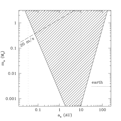
Figure 2.— The constraints on the mass (vertical axis, in unit of $M_{J}$) and orbital semi-major axis (horizontal axis, in AU) of the possible second planet placed by the Kozai migration of HD $80606$b. The shaded region must be cleared before HD $80606$b (assumed to be at $5$ AU) can undergo Kozai oscillations. The latter force HD $80606$b into a variable but highly eccentric orbit with the minimum periastron and maximum apastron delineated by the two dotted vertical lines (see Fig. 1). No planets should have survived within this region. Planets lying above the slanted dashed line would incur a radial velocity larger than $20\,\rm m/s$ on the host star (taking $\sin i=0.5$) and should have been detected were they present.

3.3. Can the Tide Raised by the Planet Account for the Residual Velocities?

NLM reported residual velocities of order $\sim 40\,\rm m/\,\rm s$ in the spectra of HD $80606$. These are higher than the expected noise and there is no clear trend in time. Could they be caused by anything other than an unknown planet? We consider one option: the tidal velocities induced by HD $80606$b on the surface of the star. The stellar rotation is ignored in the following analysis.

First, we assume that the star adjusts its hydrostatic equilibrium instantaneously according to the tidal potential of the planet at a radial separation $D=D(t)$ (the equilibrium tide picture), and estimate the corresponding tidal velocities. The maximum radial displacement at the stellar surface is roughly

$$\xi_{\rm eq}\approx{{M_{p}}\over{M_{\star}}}\left({{R_{\star}}\over D}\right)^{3}R_{\star},$$ (7)

with the horizontal displacement being of a similar order. Velocities associated with these displacements are simply estimated as $v_{\rm equi}={{d\xi_{\rm eq}}\over{dt}}$, yielding a maximum line-of-sight velocity $\sim 60{\rm cm/s}$ occurring within $10$ hours of the closest-encounter. This maximum requires conjunctions to coincide roughly with the line of periapse, as is the case in HD $80606$.

We turn next to consider a more realistic description of the tidal amplitudes. The stellar response toward the time-varying potential is decomposed into a series of eigenmode oscillations, with the mode amplitudes maximized when the tidal forcing frequencies are in resonance with the mode frequencies (the dynamical tide picture). If the planetary orbit is nearly circular, the dominant forcing frequency is $\sim 2n_{p}$. At an orbital period of $111$ days, this forcing resonantly excites gravity-modes of radial order $\sim 1000$. The spatial overlap between the tidal potential and such a high-order mode is too weak to be interesting. However, HD $80606b$ has a highly eccentric orbit. Tidal excitation occurs primarily near periastron and the dominant forcing frequencies is about twice the orbital frequency near periastron, and is related to $n_{p}$ as $\sim 2n_{p}/(1-e_{p})^{3/2}\sim 100n_{p}$. Gravity-modes of radial orders $\sim 30-80$ become relevant and their resonant excitation give rise to much larger tidal velocities. A brief treatment of the dynamical tides is given in the appendix (§B). Here we summarize our results.

Figure 3.— Dynamic response of a Sun-like star under tidal forcing from a planet of mass $3.9/\sin iM_{J}$, an orbit of period $111.82$ days and eccentricity $0.927$. We only consider the dominant $\ell=|m|=2$ component in the tidal forcing. The upper panel plots mode amplitude (in terms of surface horizontal velocity) as a function of mode period in days. Usually one or two modes dominate the response, and in this case it is a $n=41$ gravity-mode. The dotted and dashed lines are the frequency spectrum of tidal forcing over one period ($K^{1}_{\ell m}$, see appendix), and the overlap integral between the tidal potential and the eigenmode ($Q_{n\ell}$), both in arbitrary units. The forcing spectrum peaks around $2(1-e_{p})^{-3/2}n_{p}$ and the overlap integral decreases sharply when mode period (and mode radial order) increases, roughly as $Q_{n\ell}\propto n^{-5}$. Besides from these two functions, the tidal response also depends on the goodness of the resonance and the mode damping rate, these are plotted in the lower panel. The frequency detuning $\delta\sigma=|\sigma_{n}-\sigma_{j}|$. Here $\sigma_{n}$ is the frequency of a radial order $n$ mode, and $\sigma_{j}$ is the closest integer multiple of the orbital mean motion ($\sigma_{j}=jn_{p}$ and $j$ is an even number). The damping rate $\gamma_{n}$ is estimated from radiative diffusion. The two rows of short vertical bars illustrate the positions of the $\sigma_{j}$ (upper row) and $\sigma_{n}$ (lower).

We adopt the standard solar model (Christensen-Dalsgaard jorgen (1998)) to calculate the eigenmode frequencies and damping rates. The response of the star depends sensitively on how close an orbital multiple lies around one such eigenmodes. The maximum response occurs when the frequency off-resonance ($\delta\sigma$) is of order or smaller than the mode damping rate ($\gamma$), giving rise to velocities of order $10$ to $100\,\rm m/\,\rm s$. However, this is a rare event. In the frequency range of interest ($150$ to $550n_{p}$), there are roughly $N_{\rm peak}\sim 200$ discreet forcing peaks, and $N_{\rm mode}\sim 50$ eigenmodes. These modes typically have line-widths calculated from radiative diffusion to be $\gamma_{n}/\sigma_{n}\sim 10^{-7}$. A typical best resonance $\delta\sigma={\rm Min}(|\sigma_{n}-\sigma_{j}|)$ is of order $\sim n_{p}/N_{\rm mode}\sim\sigma_{n}/10^{4}\sim 10^{3}\gamma_{n}$. So the chance of one mode lying close to an orbital multiple with $\sigma_{n}\leq\gamma_{n}$ is roughly $10^{-3}$. Typical tidal velocities therefore range from $1\,\rm cm/s$ to $10\,\rm cm/s$, well below the level of the observed residues. One such example is shown in Fig. 3. The highest amplitude mode has a fractional Lagrangian pressure perturbation $\delta p/p\sim 4\times 10^{-7}$ near the surface. Translating this into light variation, this mode will be as hard to detect as the solar oscillation.

To showcase the sensitivity of the tidal responses, we plot in Fig. 4 the marked variations in the tidal responses when the orbital period is tuned through the observed uncertainty range: $111.81\pm 0.23$ days (NLM). Slight differences in the stellar structure affect the eigenmode frequencies and would also give rise to similar variations in the tidal responses. So the response results are best appreciated as a probability distribution of amplitudes, also shown in Fig. 4. We find that there is only a $\sim 10^{-3}$ chance that the tidal velocity reaches the claimed level of residues, $\sim 40\,\rm m/\,\rm s$.

Figure 4.— The probability distribution of the tidal response. The upper panel plots the horizontal velocity on the stellar surface as a function of orbital period, with the period running through the observational uncertainty range. Sharp spikes occur when an eigenmode is resonantly forced ($\delta\sigma<\gamma_{n}$). Other parameters are the same as in Fig. 3. From these data, one finds a probability distribution for the tidal velocity to surpass a certain value. This is depicted in the lower panel. Typical amplitude (probability of $0.5$) is $\sim 20\,\rm cm/s$, with the claimed level of residue, $\sim 40\,\rm m/\,\rm s$, occurring at a probability of $\sim 10^{-3}$.

We calculate the damping rates taking only radiative diffusion into account. Turbulent viscosity may enhance this damping. But this will not appreciably change our conclusion: raising the damping rates by a factor of $10$, we obtain similar results as in Fig. 4 except that high tidal amplitudes are less likely to occur.

On the other hand, when we substitute the solar model for a $1.25M_{\odot}$ ZAMS model (courtesy of Christensen-Dalsgaard), we found that the typical tidal amplitudes rise by about a factor of $10$. Equivalently, high velocity amplitudes appear roughly $10$ times more frequent. Compared to a solar model, the $1.25M_{\odot}$ model has a thinner convection zone. Its gravity-modes have a relatively larger surface amplitude.

In summary, thanks to the high eccentricity of HD $80606$b, the tidal velocities reach tantalizingly close to the current detection thresholds, but likely fail to explain any residual velocity of order $10\,\rm m/\,\rm s$. However, if the residual velocity is indeed associated with the dynamical tide, we expect it to be a coherent oscillation throughout the orbit and have a period in the range of $0.2$ to $0.6$ days. The inclination of the orbit ($\sin i$) does not affect our conclusions.

3.4. Other Planetary Systems

Figure 5.— Period versus projected mass for all observed planet candidates (http://cfa-www.harvard.edu/planets/, Sep. 2002). Circles are drawn around planets in visual binaries (Worley & Douglass worley (1997)) with a projected separation $<20\arcsec$. Besides from the 9 binaries mentioned in Zucker & Mazeh (zucker (2002), HD 142, Gl 86, HD 19994, $\epsilon$ Eri, $\tau$ Boo, HD 178911B, 16 Cyg B, HD 195019, HD 217107), there are also HD 80606, HD 213240, HD 121504, HD 46375, HD 27442, BD-103166, and $\gamma$-Cepheid. Planets lying below the dashed line incur velocity variation higher than $20\,\rm m/\,\rm s$. There appears to be an over-abundance of close-in, massive planets that are also in binaries.

Zucker & Mazeh (zucker (2002)) showed that planets in binaries are statistically different from those around isolated stars in their period-mass distribution. The former population dominates the lower-right quadrant of Fig. 5. This distinction suggests that planet migration in binaries may be induced differently from those around single stars, Kozai migration being one such possibility. Among the circled planets in Fig. 5, we have only studied $\tau$-Boo and 16 CygB. We found that $\tau$-Boo, the most massive close-in planet, could have gone through Kozai migration and later circularized, while there is no compelling evidence of Kozai migration for 16 CygB, though it could currently be undergoing Kozai oscillations (Holman et al. (holman (1997)). A binary companion may assist planet migration through other means, e.g., exciting tidal waves in the proto-planetary disk and affecting angular momentum transport. These deserve further study.

Could some of the planets around currently single stars have undergone Kozai migration followed by the subsequent disruption of the binary? We consider this unlikely. The rate of Kozai migration is limited by the tidal circularization process. For reasonable values of closest periapse distance, the latter process takes a few $10^{8}$ years or longer. By this age a typical stellar cluster has dispersed and the rate of stellar encounter has become negligible. However, it is possible that a planet’s eccentricity was excited by Kozai interaction with the binary companion before the latter was removed from the system. A simple estimate, however, finds that this may account for the observed eccentricity in at most $\sim 10\%$ of the known systems.

4. Summary

It is striking that a companion star as remote as $1000$ AU can force a planet to migrate inward. Kozai migration is a long timescale process and demands a ’clean’ planetary system in which no other planetary object exists. Kozai migration can be responsible for the present orbit of HD $80606$b only if the initial relative inclination is sufficiently high ($I\geq 85\deg$). Assuming a population of similar triple systems with randomly distributed $I$, $\sim 7\%$ of them could have gone through Kozai migration. So on the strength of one object (HD $80606$b), one may speculate about the high density of triple stellar-planetary systems yet undetected.

Our prediction regarding the lack of a second planet in the system (Fig. 2) should be tested. In this regard, we note the claim of the abnormally large residue velocities on the star. We investigated the possible association between these velocities and surface tidal waves excited by the highly eccentric planet. It seems unlikely that the latter can account for the former if the star has a structure like that of our Sun. And if the system is indeed devoid of second planet, it raises issues as to how it is cleaned.

Zucker & Mazeh (zucker (2002)) pointed out that planets in binary systems and planets around single stars do not share the same period-mass distribution. The implications might be that binaries can cause planet migration – Kozai migration being one of the more definite possibilities.

HD $80606$b’s highly elongated orbit and strong tidal interaction combine to make it a possible target for direct detection. Its current tidal luminosity (which is likely to be converted into heat and radiated all through the orbit) is $\sim 10^{28}\,\rm erg/\,\rm s$, or $\sim 14$ mag dimmer than the parent star, at a maximum angular separation of $0.01\arcsec$ (assuming distance of $80$ pc). A comparable contribution may arise if the planet evenly emits the stellar insolation it receives during periastron passages.

Appendix A Equations from EKE

We adopt the set of equations (eq. [11]-[17]) in EKE (also see Eggleton, Kiseleva & Hut EKH (1998)) to describe the secular evolution in the planet orbit, the spin of the host star and the planet. The companion is assumed to be unaffected. Physical effects described by these equations include: secular interactions, GR, tidal and rotational precessions, and tidal dissipation. These equations are explicitly listed here,

$${1\over{e_{p}}}{{de_{p}}\over{dt}} = -V_{\star}-V_{p}-5(1-e_{p}^{2})S_{eq},$$ (A1)

$${1\over{a_{p}}}{{da_{p}}\over{dt}} = -2W_{\star}-2W_{p}-{{2e_{p}^{2}}\over{1-e_{p}^{2}}}(V_{\star}+V_{p}),$$ (A2)

$${{dI}\over{dt}} = -\sin\omega_{p}\left[Y_{\star}+Y_{p}+(1-e_{p}^{2})S_{qh}\right]+\cos\omega_{p}\left[X_{\star}+X_{p}+(4e_{p}^{2}+1)S_{eh}\right],$$ (A3)

$${{d\omega_{p}}\over{dt}} = \left[Z_{\star}+Z_{p}+Z_{\rm GR}+(1-e_{p}^{2})(4S_{ee}-S_{qq})\right]-\cos\omega_{p}{{\cos I}\over{\sin I}}\left[Y_{\star}+Y_{p}+(1-e_{p}^{2})S_{qh}\right]$$ (A4)

$$-\sin\omega_{p}{{\cos I}\over{\sin I}}\left[X_{\star}+X_{p}+(4e_{p}^{2}+1)S_{eh}\right],$$

$${{d\Omega}\over{dt}} = {{\cos\omega_{p}}\over{\sin I}}\left[Y_{\star}+Y_{p}+(1-e_{p}^{2})S_{qh}\right]+{{\sin\omega_{p}}\over{\sin I}}\left[X_{\star}+X_{p}+(4e_{p}^{2}+1)S_{eh}\right],$$ (A5)

$${{d\Omega_{*\gamma}}\over{dt}} = {{\mu h_{p}}\over{I_{\star}}}(-Y_{\star}e_{\gamma}+X_{\star}q_{\gamma}+W_{\star}h_{\gamma}),$$ (A6)

$${{d\Omega_{p\gamma}}\over{dt}} = {{\mu h_{p}}\over{I_{p}}}(-Y_{p}e_{\gamma}+X_{p}q_{\gamma}+W_{p}h_{\gamma}).$$ (A7)

In eq. (A6) - (A7), the subscript $\gamma$ runs through the three spatial indexes, $E$, $Q$, and $H$, with $\hat{E}$, $\hat{Q}$, $\hat{H}$ being the three axis defining the orbital plane of the binary companion, and $\hat{e}$, $\hat{q}$ and $\hat{h}$ defining that of the planet orbit, and $e_{E}=\hat{e}\cdot\hat{E}$, etc. The inclination $I$ is taken to be that between the two planes, with the binary plane held constant during the evolution. The other two angles, $\omega_{p}$ and $\Omega$, are the argument of the planet pericentre, and the longitude of the planet ascending node, respectively. The spin vector $\Omega_{\star}$ ($\Omega_{p}$) belongs to the host star (planet), and $I_{\star}=r_{g\star}M_{\star}R_{\star}^{2}$ is the stellar moment of inertia, with $r_{g\star}$ typically called the gyro-radius. $I_{p}$ is for the planet. The planet orbit has an angular momentum of magnitude $h_{p}=[G(M_{\star}+M_{p})a_{p}(1-e_{p}^{2})]^{1/2}$, and the reduced mass of the planet-star system is $\mu=M_{\star}M_{p}/(M_{\star}+M_{p})$. All other symbols are defined in EKE. We do not repeat these definitions here.

We introduce two commonly used dimensionless numbers, $k_{2}$ (the tidal Love number) and $Q$ (the tidal quality factor), and relate them to the notation in EKE,

$$A_{\star}=k_{2\star}R_{\star}^{5}, A_{p}=k_{2p}R_{p}^{5},$$ (A8)

$${1\over{t_{F\star}}}={{3k_{2\star}}\over{Q_{\star}}}\left({{R_{\star}}\over{a_{p}}}\right)^{5}{{M_{p}}\over{M_{\star}}}\,n_{p}, {1\over{t_{Fp}}}={{3k_{2p}}\over{Q_{p}}}\left({{R_{p}}\over{a_{p}}}\right)^{5}{{M_{\star}}\over{M_{p}}}\,n_{p}.$$ (A9)

Appendix B Dynamical Tide

We provide a simple description of the dynamical tide treatment. The final results are presented in §3.3.

The period of the stellar spin is likely long compared to both the sound crossing time and the dominant tidal forcing period. So we assume a non-rotating star. Following Press & Teukolsky (press (1977)) and Lai (donglai (1997)) and notations therein, we decompose the tidal potential at a point ${\bf r}=[r,\theta,\phi]$ inside the star, due to a planet at location ${\bf D}(t)=[D(t),\pi/2,f(t)]$, as

$$U({\bf r},t)=-GM_{p}\sum_{\ell,m}W_{\ell m}{{r^{\ell}}\over{D^{\ell+1}}}Y_{\ell m}(\theta,\phi)\exp^{-imf(t)}.$$ (B1)

The stellar fluid responds with a displacement ${\bf\xi}({\bf r},t)$ which can be projected onto various free eigen-oscillations,

$${\bf\xi}({\bf r},t)=\sum_{\alpha}a_{\alpha}(t){\bf\xi}_{\alpha}({\bf r}).$$ (B2)

The eigenfunctions are normalized as $\int d^{3}x\rho{\bf\xi}_{\alpha}\cdot{\bf\xi}_{\alpha}^{*}=1$. We denote the mode eigenfrequency as $\sigma_{\alpha}$ and damping rate as $\gamma_{\alpha}$, and introduce ${\tilde{a}}_{\alpha}(\sigma)$ which is related to $a_{\alpha}(t)$ by

$$\hskip 28.45274pta_{\alpha}(t)=\int_{0}^{\infty}d\sigma\exp^{-i\sigma t}{\tilde{a}}_{\alpha}(\sigma).$$ (B3)

Substituting equation (B2) into the fluid equation of motion, we obtain

$${\tilde{a}}_{\alpha}(\sigma)={1\over{\sigma_{\alpha}^{2}-\sigma^{2}+2i\gamma_{\alpha}\sigma}}\sum_{\ell}{{GM_{p}}\over{D_{p}^{\ell+1}}}Q_{\alpha\ell}K_{\ell m}(\sigma),$$ (B4)

where the periapse distance $D_{p}=a_{p}(1-e_{p})$, $K_{\ell m}(\sigma)$ is the frequency spectrum for the $Y_{\ell m}$ component of the tidal potential, and $Q_{\alpha\ell}$ is the spatial overlap integral between the tidal forcing and the $\alpha$ eigenfunction,

$$K_{\ell m}(\sigma) = {{W_{\ell m}}\over{2\pi}}\int^{\infty}_{0}dt\left[{{D_{p}}\over{D(t)}}\right]^{\ell+1}\exp[-imf(t)+i\sigma t],$$ (B5)

$$Q_{\alpha\ell} = \int d^{3}x\,\,\rho{\bf\xi}_{\alpha}^{*}\cdot\nabla(r^{\ell}Y_{\ell m})=\int d^{3}x\,\,\rho_{\alpha}^{\prime*}\,r^{\ell}Y_{\ell m}.$$ (B6)

Here, $\rho_{\alpha}^{\prime}$ is the Eulerian density perturbation for mode $\alpha$. The continuity equation gives $\nabla\cdot(\rho\xi_{\alpha})=-\rho_{\alpha}^{\prime}$.

We first focus on $K_{\ell m}$. For a strictly periodic orbit, $K_{\ell m}(\sigma)$ equals a sum of delta functions with non-zero values only at the integer multiples ($j$) of the orbital mean motion.

$$K_{\ell m}(\sigma)=\sum_{j=0}^{\infty}C_{j}(\sigma)\,\delta(\sigma-jn_{p}).$$ (B7)

To obtain $C_{j}$, we calculate the tidal spectrum integrated over one orbital period,

$$K^{1}_{\ell m}(\sigma)={{W_{\ell m}}\over{2\pi}}\int_{0}^{2\pi/n_{p}}dt\left[{{D_{p}}\over{D(t)}}\right]^{\ell+1}\exp[-imf(t)+i\sigma t].$$ (B8)

Unlike $K_{\ell m}$, this quantity is a smooth function of frequency. For $\ell=|m|=2$, the forcing maximum lies around $\sigma\sim(1-e_{p})^{-3/2}|m|n_{p}$, i.e., $\sigma\sim 2n_{p}$ for $e_{p}\ll 1$ and $\sigma\sim 90n_{p}$ for $e_{p}=0.927$. This is shown in Figure 3. When integration in $K_{\ell m}$ is carried out over $N$ number of orbital cycles, the resulting forcing spectrum can be approximately described by the following log-normal distribution,

$$K^{N}_{\ell m}(\sigma)=\sum_{j=1}^{\infty}N\exp\left[-({\sigma\over{n_{p}}}-j)^{2}N^{2}\right]\,K^{1}_{\ell m}(\sigma).$$ (B9)

And when $N\rightarrow\infty$, we retrieve $K_{\ell m}$ with $C_{j}(\sigma)=\sqrt{\pi}n_{p}K_{\ell m}^{1}(\sigma)$

Substituting the above expression for $K_{\ell m}(\sigma)$ into equations (B2)- (B4), we obtain the mode amplitude,

$$a_{\alpha}(t)\approx{{GM_{p}}\over{D_{p}^{\ell+1}}}\sqrt{\pi}n_{p}\,Q_{\alpha\ell}K^{1}_{\ell m}(\sigma_{j})\int_{(j-{1\over 2})n_{p}}^{(j+{1\over 2})n_{p}}d\sigma\,{{\delta(\sigma-jn_{p})e^{-i\sigma t}}\over{\sigma_{\alpha}^{2}-\sigma^{2}+2i\gamma_{\alpha}\sigma}}={{GM_{p}}\over{D_{p}^{\ell+1}}}\sqrt{\pi}n_{p}\,Q_{\alpha\ell}K^{1}_{\ell m}(\sigma_{j}){{e^{-i\sigma_{j}t}}\over{\sigma_{\alpha}^{2}-\sigma_{j}^{2}+2i\gamma_{\alpha}\sigma_{j}}},$$ (B10)

where $\sigma_{j}=jn_{p}$ is the closest orbital multiples to the mode frequency $\sigma_{\alpha}$.

The value of the tidal overlap, $Q_{\alpha\ell}$, decays sharply with both $\ell$ and the radial order ($n$) of the mode. For a high order gravity-mode, most of the net contribution to $Q_{\alpha\ell}$ comes from the upper evanescent region of the mode – the bottom of the surface convection zone where $\rho^{\prime}/\rho$ is fairly constant. We find that $Q_{\alpha\ell}$ scales with $n$ as

$$Q_{\alpha\ell}\propto n^{-5}.$$ (B11)

References

- (1) Batten, A. H.; Fletcher, J. M.; MacCarthy, D. G. 1989, Victoria: Dominion Astrophysical Observatory,
- (2) Blaes, O., Lee, M. H., Socrates, A., 2002, ApJ,578,775
- (3) Drake, S. A.; Pravdo, S . H.; Angelini, L.; Stern, R. A. 1998, AJ, 115, 2122
- (4) Duquennoy, A.; Mayor, M. 1991, A&A, 248, 485
- (5) Duquennoy, A.; Mayor, M.; Andersen, J.; Carquillat, J. M.; North, P. 1992, A&A, 254,13
- (6) Eggleton, P. P., Kiseleva, L. G., & Hut, P. 1998, ApJ, 499, 853
- (7) Eggleton, P. P., & Kiseleva-Eggleton, L. G., 2001, ApJ, 562, 1012
- (8) Einstein, A. 1916, Annalen der Physik, Band 49, 50
- (9) Ford, E. B.; Kozinsky, B.; Rasio, F. A. 2000,ApJ,535,385
- (10) Ford, E. B.; Havlickova, M.; Rasio, F. A. 2001, Icarus, 150, 303
- (11) Goldreich, P.; Nicholson, P. D. 1989,ApJ,342,1079
- (12) Goldreich, P.; Sari, R. 2002, astro-ph/0202462 (submitted to ApJ)
- (13) Goldreich, P.; Soter, S. 1966, Icarus, 5, 375
- (14) Goldreich, P.; Tremaine, S., 1980, ApJ, 241, 425
- (15) Griffin, R. F.; Griffin, R. E. M.; Gunn, J. E.; Zimmerman, B. A. 1985, AJ, 90, 609
- (16) Holman, M., Touma, J., & Tremaine, S. 1997, Nature, 386, 254
- (17) Hut, P. 1981, A&A, 99, 126
- (18) Innanen, K. A.; Zheng, J. Q.; Mikkola, S.; Valtonen, M. J., 1997, AJ, 113, 1915
- (19) Christensen-Dalsgaard, J. ;.1998, Space Science Reviews, 85, 19
- (20) Lin, D. N. C.; Bodenheimer, P.; Richardson, D. C, 1996, Nature, 380, 606
- (21) Kiseleva, L. G., Eggleton, P. P.,& Mikola, S. 1998, MNRAS, 300, 292
- (22) Kozai, Y. 1962, AJ, 67, 591
- (23) Lai, D. 1997, ApJ, 490, 847
- (24) Mazeh, T., Krymolowski, Y. Rosenfeld, G., 1997, ApJ, 477L, 103
- (25) Murray, C.D., Dermott, S.F., Solar System Dynamics, Cambridge University Press, 2000, MD2000
- (26) Naef, D.; Latham, D. W.; Mayor, M. et al. 2001, A&A, 375, L27 NLM
- (27) Peale, S. J.; Greenberg, R. J. 1980, LPI, 11, 871
- (28) Press, W. H.; Teukolsky, S. A. 1977, ApJ, 213, 183
- (29) Sterne, T.E. 1939, MNRAS, 99, 451
- (30) Worley, C. E.; Douglass, G. G. 1997, A&AS, 125, 523
- (31) Wu, Y. 2002, in Scientific Frontiers in Research on exo-solar Planets, eds. Deming, D., Seager, S., PASP
- (32) Zucker, S.; Mazeh, T. 2002,ApJ, 568, 113