Exploring the Expanding Universe and Dark Energy using the Statefinder Diagnostic

Abstract

The coming few years are likely to witness a dramatic increase in high quality Sn data as current surveys add more high redshift supernovae to their inventory and as newer and deeper supernova experiments become operational. Given the current variety in dark energy models and the expected improvement in observational data, an accurate and versatile diagnostic of dark energy is the need of the hour. This paper examines the Statefinder diagnostic in the light of the proposed SNAP satellite which is expected to observe about 2000 supernovae per year. We show that the Statefinder is versatile enough to differentiate between dark energy models as varied as the cosmological constant on the one hand, and quintessence, the Chaplygin gas and braneworld models, on the other. Using SNAP data, the Statefinder can distinguish a cosmological constant ($w=-1$) from quintessence models with $w\geq-0.9$ and Chaplygin gas models with $\kappa\leq 15$ at the $3\sigma$ level if the value of $\Omega_{m}$ is known exactly. The Statefinder gives reasonable results even when the value of $\Omega_{m}$ is known to only $\sim 20\%$ accuracy. In this case, marginalizing over $\Omega_{m}$ and assuming a fiducial LCDM model allows us to rule out quintessence with $w\geq-0.85$ and the Chaplygin gas with $\kappa\leq 7$ (both at $3\sigma$). These constraints can be made even tighter if we use the Statefinders in conjunction with the deceleration parameter. The Statefinder is very sensitive to the total pressure exerted by all forms of matter and radiation in the universe. It can therefore differentiate between dark energy models at moderately high redshifts of $z\lower 3.87495pt\hbox{ $\buildrel<\over{\sim}$}~{}10$.

1 Introduction

Supernova observations (Riess et al. , 1998; Perlmutter et al. , 1999), when combined with those of the cosmic microwave background (Benoit et al. , 2003) and gravitational clustering (Percival, 2002), suggest that our Universe is (approximately) spatially flat and that an exotic form of negative-pressure matter called ‘dark energy’ (DE) causes it to accelerate by contributing as much as 2/3 to the closure density of the universe – the remaining third consisting of non-relativistic dark matter and baryons. The simplest example of dark energy is the cosmological constant ($\Lambda$), with associated mass density

$$\rho_{\Lambda}=6.44\times 10^{-30}\left({\Omega_{\Lambda}\over 0.7}\right)\left({h\over 0.7}\right)^{2}{\rm{g~{}cm^{-3}}}\,\,,$$ (1)

where $h$ is the Hubble constant $H_{0}$ in terms of $100$ km s^-1 Mpc^-1 and $\Omega_{\Lambda}=0.7\pm 0.1,~{}h=0.7\pm 0.1$. Although the cold dark matter model with a cosmological constant (hereafter LCDM) provides an excellent explanation for the acceleration phenomenon and other existing observational data, it remains entirely plausible that the dark energy density is weakly time dependent (see the reviews Sahni & Starobinsky, 2000; Peebles & Ratra, 2003). Moreover, it is natural to suggest (in complete analogy with what has been done in the case of another type of ‘dark energy’ responsible for driving the expansion of the universe during an inflationary stage in the early universe) that the dark energy which we observe today might really be dynamical in nature and origin. This means that a completely new form of matter is responsible for giving rise to the second inflationary regime which we are entering now.

Many models of dark energy have been proposed; in fact, any inflationary model (even a ‘bad’ one, i.e. without a ‘graceful exit’ to the subsequent radiation-dominated Friedmann-Robertson-Walker (FRW) stage) may be used for this purpose if one assumes different values for its microscopic parameters. The simplest of these models rely on a scalar field minimally interacting with Einstein gravity – quintessence (Ratra & Peebles, 1988; Peebles & Ratra, 1988; Frieman et al. , 1995; Caldwell, Dave & Steinhardt, 1998), and bear an obvious similarity with the simplest variants of the inflationary scenario. Inclusion of a non-minimal coupling to gravity in these models together with further generalization leads to models of dark energy in a scalar-tensor theory of gravity (see Boisseau et al. , 2000, and references therein). Other models invoke matter with unusual properties such as the Chaplygin gas (Kamenshchik, Moschella & Pasquier, 2001) or k-essence (Armendariz-Picon, Mukhanov & Steinhardt, 2000). Still others generate cosmic acceleration through topological defects (Bucher & Spergel, 1999) or quantum vacuum polarization and particle production (Sahni & Habib, 1998; Parker & Raval, 1999). Lately it has been noticed that higher dimensional ‘braneworld’ models could account for a late-time accelerating phase even in the absence of matter violating the strong energy condition (Dvali, Gabadadze & Porrati, 2000; Deffayet, Dvali & Gabadadze, 2002; Deffayet et al. , 2002; Sahni & Shtanov, 2002; Alam & Sahni, 2002) (see Sahni, 2002, for a recent review of dark energy models). It is especially interesting that in the latter class of models ’dark energy’ need not be an energy of some form of matter at all, but can have an entirely geometrical origin. Moreover, in these models the basic gravitational field equations do not have the Einstein form

$$R_{\alpha\beta}-{{1\over 2}}g_{\alpha\beta}R=8\pi G\left(T_{\alpha\beta}\big{|}_{\mathit{m}atter}+T_{\alpha\beta}\big{|}_{\mathit{r}adiation}+T_{\alpha\beta}\big{|}_{\mathit{D}E}\right)$$ (2)

($c=\hbar=1$ is assumed here and below), and therefore the notions of ‘energy density’ and ‘pressure’ of DE loose their exact fundamental sense and become ambiguous and convention-dependent. A major ambiguity arises in models of scalar-tensor gravity as well as in braneworld models both of which contain interaction terms between dark energy and non-relativistic matter. Interpreting such models within the Einstein framework (2) leads to the following dilemma: should these interaction terms be ascribed to dark matter (hence to $T_{\alpha\beta}|_{\mathit{m}atter}$ in (2)) or to dark energy (to $T_{\alpha\beta}|_{\mathit{D}E}$) ? Our answer to this question has the potential to alter the properties of dark energy including its density and pressure and hence also its equation of state. In marked contrast to such ambiguities which could arise if we are not careful with our usage of the term ‘equation of state’, the expansion factor of the universe in the physical frame $a(t)$, when expressed through the Hubble parameter $H\equiv{\dot{a}\over a}$, is an unambiguous, fundamental and readily measurable quantity.

Given the rapidly improving quality of observational data and also the abundance of different theoretical models of dark energy, the need of the hour clearly is a robust and sensitive statistic which can succeed in differentiating cosmological models with various kinds of dark energy both from each other and, even more importantly, from an exact cosmological constant. In view of the non-fundamentality of the notions of DE density and pressure pointed out above, we prefer to work with purely geometric quantities. Then such a sensitive diagnostic of the present acceleration epoch and of dark energy could be the statefinder pair $\{r,s\}$, recently introduced in Sahni et al.  (2003). The statefinder probes the expansion dynamics of the universe through higher derivatives of the expansion factor ${\ddot{a}}~{}\&\stackrel{{\scriptstyle...}}{{a}}$. Its important property is that $\{r,s\}=\{1,0\}$ is a fixed point for the flat LCDM FRW cosmological model. Departure of a given DE model from this fixed point is a good way of establishing the ‘distance’ of this model from flat LCDM. As we will show in this paper, the statefinder successfully differentiates between rival DE models and, when combined with SNAP supernova data, can serve as a versatile and powerful diagnostic of dark energy.

The paper is organized as follows. In the next section we briefly review some theoretical models of dark energy. The behaviour of the statefinder pair for these models is discussed in Section III while the nature of data expected to become available from the SNAP experiment is the subject of Section IV. Section IV also discusses model-independent parametric reconstructions of dark energy. Our conclusions are presented in section V.

2 Dark energy models and the acceleration of the universe

The rate of expansion of a FRW universe and its acceleration are described by the pair of equations

$$H^{2} = \frac{8\pi G}{3}\sum_{i}\rho_{i}-\frac{k}{a^{2}}~{},$$

$$\frac{\ddot{a}}{a} = -\frac{4\pi G}{3}\sum_{i}(\rho_{i}+3p_{i}),$$ (3)

where the summation is over all matter fields contributing to the dynamics of the universe. Clearly a necessary (but not sufficient) condition for acceleration (${\ddot{a}}>0$) is that at least one of the matter fields in (2) violate the strong energy condition $\rho+3p\geq 0$. If for simplicity we assume that the dark energy pressure and density are related by the simple linear relation $p=w\rho$, then $w<-1/3$ is a necessary condition for the universe to accelerate. The acceleration of the universe can be quantified through a dimensionless cosmological function known as the ‘deceleration parameter’ $q=-{\ddot{a}}/aH^{2}$, equivalently

$$q(x)=\frac{H^{\prime}(x)}{H(x)}~{}x-1\,,~{}~{}~{}x=1+z\,,$$ (4)

where $q<0$ describes an accelerating universe, whereas $q\geq 0$ for a universe which is either decelerating or expanding at the ‘coasting’ rate $a\propto t$. As it will soon be shown, the deceleration parameter on its own does not characterize the current accelerating phase uniquely. The presence of a fairly large degeneracy in $q(z)$ is reflected in the fact that rival dark energy models can give rise to one and the same value of $q_{0}$ at the present time. This degeneracy is easily broken if, as demonstrated in section 3, one combines $q(z)$ with one of the statefinders $r(z)$, $s(z)$. The diagnostic pairs $\{r,q\}$ and $\{s,q\}$ provide a very comprehensive description of the dynamics of the universe and consequently of the nature of dark energy.

Now let us come to the issue of defining the energy density and pressure of DE. In view of the ambiguities discussed in the Introduction, we shall define $\rho_{\rm DE}$ and $p_{\rm DE}$ by making use of the Einstein interpretation of gravitational field equations (not to be confused with the notion of the Einstein frame which is used in scalar-tensor and string theories of gravity!). Namely, we assume that the gravitational field equations in a single-metric theory of 3+1 gravity can be formally written in the form (2) where the Einstein tensor standing in the left-hand side is defined with respect to the physical space-time metric. All other terms are transferred to the right-hand side. Next, we subtract the energy-momentum tensor of dust (CDM + baryons) from the total energy-momentum tensor of matter and call the remaining part ‘the effective energy-momentum tensor of dark energy’ (in the Einstein interpretation). Combining this prescription with Eq. (2) and in the absence of spatial curvature, the energy density and pressure of dark energy can be defined as:

$$\rho_{\rm DE} = \rho_{\rm critical}-\rho_{\rm m}=\frac{3H^{2}}{8\pi G}(1-\Omega_{\rm m})~{},$$

$$p_{\rm DE} = \frac{H^{2}}{4\pi G}(q-\frac{1}{2})~{},$$ (5)

where $\rho_{\rm critical}=3H^{2}/8\pi G$ is the critical density associated with a FRW universe. An important consequence of using this approach is that the ratio $w_{DE}\equiv p_{DE}/\rho_{DE}$ can be expressed in terms of the deceleration parameter

$$w_{\rm eff}(x)={2q(x)-1\over 3\left(1-\Omega_{\rm m}(x)\right)}\equiv\frac{(2x/3)\ d\ {\rm ln}H\ /\ dx-1}{1\ -\ (H_{0}/H)^{2}\Omega_{m}\ x^{3}}\,\,.$$ (6)

Following the above prescription we get standard results for the cosmological constant and quintessence (for instance we recover Eq. (• ‣ 2)). However the same cannot be said of braneworld models since the Hubble parameter for the latter contains interaction terms between matter and dark energy (see for instance Eqs. (22), (23)) and therefore does not subscribe to the Einsteinian format (2) & (2). One can however extend the above definition of $w_{\rm eff}$ to non-Einsteinian theories by defining dark energy density to be the remainder term after one subtracts the matter density from the critical density in the Einstein equations. It should be emphasised that, according to this prescription all interaction terms between matter and dark energy (such terms arise in scalar-tensor and brane models) are attributed solely to dark energy. Therefore $w_{\rm eff}(z)$ defined according to (6) is an effective equation of state in these models and not a fundamental physical entity (as it is in LCDM, for instance).

In this connection we should also stress that the propagation velocity of small inhomogeneities in dark energy is generically neither $\sqrt{w_{DE}}$, nor $\sqrt{dp_{DE}/d\rho_{DE}}$. Therefore although $w(z)$ is an important physical quantity it does not provide us with an exhaustive description of dark energy and its use as a diagnostic should be treated with some caution. (In this paper we will restrict ourselves to a spatially flat FRW model and will not consider inhomogeneous perturbations on this background.)

We now highlight a few popular candidates for dark energy which shall be the focus of our discussion in this paper.

• Cosmological Constant. Perhaps the simplest model for dark energy is a cosmological constant $\Lambda$, whose energy density remains constant with time $\rho_{\Lambda}\equiv\Lambda/8\pi G=-p_{\Lambda}$, and which has an equation of state $w_{\Lambda}=-1$. A universe consisting of matter in the form of dust and the cosmological constant is popularly known as LCDM, the Hubble parameter for this model has the form

  $$H(z)=H_{0}\left[\Omega_{\rm m}(1+z)^{3}+1-\Omega_{\rm m}\right]^{1/2}~{}.$$ (7)

• Quiessence. The next simplest form of dark energy after the cosmological constant is provided by models for which the equation of state is a constant $w={\rm constant}\neq-1$. For this form of dark energy, which we call ‘quiessence’

  $$H(z)=H_{0}\left[\Omega_{\rm m}(1+z)^{3}+\Omega_{X}(1+z)^{3(1+w)}\right]^{1/2}~{}.$$ (8)

  For $w=-1$ we recover the limiting form (7). Important examples of quiessence include a network of non-interacting cosmic strings ($w=-1/3$) and domain walls ($w=-2/3$). Quiessence in a FRW universe can also be produced by a scalar field (quintessence) which has the potential $V(\phi)\propto\sinh^{{-2(1+w)\over w}}(C\phi+D)$, with appropriately chosen values of $C$ and $D$ (see Sahni & Starobinsky, 2000; Urena-Lopez & Matos, 2000).

  Usually the dark energy equation of state depends upon time. We call such more generic models kinessence.

• Quintessence The simplest example of kinessence is provided by quintessence – a self-interacting scalar field which couples minimally to gravity. Its density, pressure and equation of state are given by

  $$\rho_{\phi} = {1\over 2}\dot{\phi}^{2}+V(\phi),~{}~{}p_{\phi}={1\over 2}\dot{\phi}^{2}-V(\phi),$$

  $$w_{\phi} = \frac{p_{\phi}}{\rho_{\phi}}=\frac{{1\over 2}\dot{\phi}^{2}-V(\phi)}{{1\over 2}\dot{\phi}^{2}+V(\phi)}\geq-1\,\,.$$ (9)

  Scalar field evolution is governed by the equation of motion

  $$\ddot{\phi}+3H\dot{\phi}+\frac{dV}{d\phi}=0~{},$$ (10)

  where

  $$H^{2}=\frac{8\pi G}{3}\left[\rho_{0m}(1+z)^{3}+{1\over 2}{\dot{\phi}}^{2}+V(\phi)\right].$$ (11)

  It is clear from (• ‣ 2) that $w<-1/3$ provided $\dot{\phi}^{2}<V(\phi)$. Models with this property can lead to an accelerating universe at late times. An important subclass of quintessence models displays the so-called ‘tracker’ behaviour during which the ratio of the scalar field energy density to that of the matter/radiation background changes very slowly over a substantial period of time. Models belonging to this class satisfy $V^{\prime\prime}V/(V^{\prime})^{2}\geq 1$ and approach a common evolutionary ‘tracker path’ from a wide range of initial conditions. As a result, the present value of dark energy in tracker models is to a large extent (though not entirely) independent of initial conditions and is determined by parameters residing only in its potential – as in the case of the cosmological constant (for a brief review of tracker models see Sahni, 2002). In this paper we will focus our attention on the tracker potential $V(\phi)\propto\phi^{-\alpha}$, $\alpha\geq 1$ which was originally proposed in Ratra & Peebles (1988). For this potential, the region of initial conditions for $\phi$ for which the tracker regime has been reached before the end of the matter-dominated stage is $\phi_{in}\ll M_{P}\equiv 1/\sqrt{G}$, and the present value of quintessence is $\phi(t_{0})\sim M_{P}$.

  For all quintessence models $w\geq-1$, and this inequality is saturated only if $\dot{\phi}=dV/d\phi=0$. In order to obtain $w<-1$ matter must violate the strong energy condition $\rho+3p\geq 0$, for some duration of time. It should be noted that DE with $w<-1$ is not excluded by observations (see Melchiorri et al. , 2002, for a recent investigation). However in order to have $w<-1$ one must look beyond quintessence models. Models based on scalar-tensor gravity (Boisseau et al. , 2000) can have $w<-1$, so too can braneworld models (see Sahni & Shtanov 2002 for a discussion of this issue and Alam & Sahni 2002 for a comparison of braneworld models with observational data).

• Chaplygin gas. An interesting alternate form of dark energy is provided by the Chaplygin gas (Kamenshchik et al. 2001; Bilic, Tupper & Viollier, 2002; Fabris, Goncalves & de Souza, 2002; Gorini, Kamenshchik & Moschella, 2003; Alcaniz, Jain & Dev, 2003; Avelino et al. , 2003) which obeys the equation of state

  $$p_{c}=-A/\rho_{c}~{}.$$ (12)

  The energy density of the Chaplygin gas evolves according to

  $$\rho_{c}=\sqrt{A+B(1+z)^{6}}\,\,,$$ (13)

  from where we see that $\rho_{c}\to\sqrt{A}$ as $z\to-1$ and $\rho_{c}\to\sqrt{B}(1+z)^{3}$ as $z\gg 1$. Thus, the Chaplygin gas behaves like pressureless dust at early times and like a cosmological constant during very late times. Note, however, that Chaplygin gas at $z\gg 1$ is not simply a new kind of CDM if we examine its inhomogeneities ( i.e. if we apply this hydrodynamical equation of state to the inhomogeneous case, too)! In contrast to CDM and baryons, the sound velocity in the Chaplygin gas $v_{c}=\sqrt{dp_{c}/d\rho_{c}}={\sqrt{A}/\rho_{c}}$ quickly grows $\propto t^{2}$ during the matter-dominated stage and becomes of the order of the velocity of light at present (it approaches light velocity asymptotically in the distant future ). Thus, from the point of view of inhomogeneities, the properties of the Chaplygin gas during the matter-dominated epoch are very unusual and resemble those of hot dark matter which has a large Jeans length, despite the fact that the Chaplygin gas formally carries negative pressure.

  The Hubble parameter for a universe containing cold dark matter and the Chaplygin gas is given by

  $$H(z)=H_{0}\left[\Omega_{m}(1+z)^{3}+\frac{\Omega_{m}}{\kappa}\sqrt{\frac{A}{B}+(1+z)^{6}}\right]^{1/2}\,\,,$$ (14)

  where $\kappa=\rho_{0m}/\sqrt{B}$. It is easy to see from (14) that

  $$\kappa=\frac{\rho_{0m}}{\rho_{c}}(z\to\infty)\,\,.$$ (15)

  Thus, $\kappa$ defines the ratio between CDM and the Chaplygin gas energy densities at the commencement of the matter-dominated stage. It is easy to show that

  $$A=B\left\{\kappa^{2}\left(\frac{1-\Omega_{m}}{\Omega_{m}}\right)^{2}-1\right\}\,\,.$$ (16)

  In the limiting case when $A=0$, the Chaplygin gas becomes indistinguishable from dust-like matter (if we examine its behaviour in an unperturbed FRW background). This limiting case corresponds to

  $$\kappa=\frac{\Omega_{m}}{1-\Omega_{m}}\,\,,$$ (17)

  and is shown as the outer envelope (dashed) to the Chaplygin gas models in Figures 1a,b. In the other limiting case $B=0$, the Chaplygin gas reduces to the cosmological constant.

  The fact that the sound velocity in the Chaplygin gas is not small during the matter-dominated stage and becomes very large towards its end suggests that the parameter $\kappa$ should be large in order to avoid damping of adiabatic perturbations. This requires $A\gg B$. Recent investigations which look at Chaplygin gas models in the light of galaxy clustering data and CMB anisotropies show that this observation is correct if the equation of state $p_{c}\propto-1/\rho_{c}$ is assumed to be universally valid (Carturan & Finelli, 2002; Sandvik et al. , 2002; Bean & Dore, 2003). In our paper we consider the Chaplygin gas equation of state to be a phenomenological description of dark energy in a FRW background and do not assume that it remains true for perturbations. However, the fact that $\kappa$ should be large for viable models will appear in our results, too. Finally let us point out that the Chaplygin gas may be considered to be a specific case of k-essence with a constant potential and the Born-Infeld kinetic term. To illustrate this consider the Born-Infeld lagrangian density

  $${\cal L}=-V_{0}\sqrt{1-\phi_{,\mu}\phi^{,\mu}}~{},$$ (18)

  where $\phi_{,\mu}\equiv\partial{\phi}/\partial x^{\mu}$. For time-like $\phi_{,\mu}$ one can define a four velocity

  $$u^{\mu}=\frac{\phi^{,\mu}}{\sqrt{\phi_{,\alpha}\phi^{,\alpha}}}~{},$$ (19)

  this leads to the standard form for the hydrodynamical energy-momentum tensor

  $$T_{\mu\nu}=(\rho+p)u_{\mu}u_{\nu}-pg_{\mu\nu}~{},$$ (20)

  where (Frolov, Kofman & Starobinsky, 2002)

  $$\rho=\frac{V_{0}}{\sqrt{1-\phi_{,\mu}\phi^{,\mu}}}~{},~{}~{}p=-V_{0}\sqrt{1-\phi_{,\mu}\phi^{,\mu}}~{},$$ (21)

  and we find that we have recovered (12) with $A=V_{0}^{2}$.

• Braneworld models. Braneworld models provide an interesting alternative to dark energy model building. According to this higher dimensional world view, we live on a 3+1 dimensional brane (‘brane’ being a multidimensional generalization of ‘membrane’) which is either embedded in or bounds a higher dimensional space-time. The simplest example of a braneworld which can lead to late-time acceleration is the model suggested by Deffayet et al. (2002) (we shall henceforth refer to this model as the DDG model).

  $$H=\sqrt{\frac{8\pi G\rho_{\rm m}}{3}+\frac{1}{l_{c}^{2}}}+\frac{1}{l_{c}}~{},$$ (22)

  where $l_{c}=m^{2}/M^{3}$ is a new length scale and $m$ and $M$ refer respectively to the four and five dimensional Planck mass ($l_{c}=2r_{c}$ in the terminology of Deffayet et al. 2002). The acceleration of the universe in this model is not caused by the presence of ‘dark energy’ but due to the fact that general relativity is formulated in 5 dimensions instead of the usual 4. One consequence of this is that gravity becomes five dimensional on length scales $R>l_{c}=2H_{0}^{-1}(1-\Omega_{\rm m})^{-1}$. A more general class of braneworld models is described by (Sahni & Shtanov, 2002)

  $${H^{2}(z)\over H_{0}^{2}} = \Omega_{\rm m}(1\!+\!z)^{3}+\Omega_{\sigma}+\underline{2\Omega_{l}\mp}$$ (23)

  $$\underline{2\sqrt{\Omega_{l}}\,\sqrt{\Omega_{\rm m}(1\!+\!z)^{3}+\Omega_{\sigma}+\Omega_{l}+\Omega_{\Lambda_{\rm b}}}}\,,$$

  where $\Lambda_{\rm b}$ is the bulk cosmological constant, $\sigma$ is the brane tension and

  $$\Omega_{\rm m}={\rho_{0m}\over 3m^{2}H_{0}^{2}},\Omega_{\sigma}={\sigma\over 3m^{2}H_{0}^{2}},\Omega_{l}={1\over l_{c}^{2}H_{0}^{2}},\Omega_{\Lambda_{\rm b}}=-{\Lambda_{\rm b}\over 6H_{0}^{2}}$$ (24)

  It is easy to see that $l_{c}$ can be of the same order as the Hubble radius $l_{c}\sim H_{0}^{-1}$ if $M\sim 100$ MeV. On short length scales $r\ll l_{c}$ and at early times, one recovers general relativity, whereas on large length scales $r\gg l_{c}$ and at late times brane-related effects begin to play an important role. It is interesting that brane-inspired effects can lead to the late time acceleration of the universe even in the complete absence of a matter source which violates the strong energy condition $\rho+3p\geq 0$ (Deffayet et al. 2002; Sahni & Shtanov, 2002).

  The dimensionless value of the brane tension $\Omega_{\sigma}$ is determined by the constraint relation

  $$\Omega_{\rm m}+\Omega_{\sigma}\mp\underline{2\sqrt{\Omega_{l}}\,\sqrt{1-\Omega_{\kappa}+\Omega_{\Lambda_{\rm b}}}}=1.$$ (25)

  The underlined terms in (23) & (25) make braneworld models different from standard FRW cosmology. Indeed by setting $\Omega_{l}=0$ (23) reduces to the LCDM model

  $${H^{2}(z)\over H_{0}^{2}}=\Omega_{\rm m}(1\!+\!z)^{3}+\Omega_{\sigma}$$ (26)

  which describes a universe containing matter and a cosmological constant (7). The two signs in (23) correspond to the two separate ways in which the brane can be embedded in the higher dimensional bulk. As shown in Sahni & Shtanov (2002), taking the upper sign in (23) and (25) leads to the model called BRANE1, while the lower sign in (23) and (25) results in BRANE2.

  Three important classes of braneworld models deserve special mention:

  1. BRANE1 models have an effective equation of state which is more negative than that of the cosmological constant $w\leq-1$.

  2. BRANE2 models have $w\geq-1$. For parameter values $\Omega_{\sigma}=\Omega_{\Lambda_{\rm b}}=0$, BRANE2 coincides with the dark energy model discussed in Eq. (22).

  3. A class of braneworld models, called ‘disappearing dark energy’ (DDE) (Sahni & Shtanov, 2002; Alam & Sahni, 2002), have the important property that the current acceleration of the universe is a transient phase which is sandwiched between two matter dominated epochs. These models do not have horizons and therefore help to reconcile an accelerating universe with the demands of the string/M-theory (Sahni, 2002) (as well as any theory which requires dark energy to decay in the future and transform into matter with $w\geq-1/3$).

  Finally we note that, for a spatially flat universe, the luminosity distance for all models discussed above is given by the simple expression

  $$\frac{D_{L}(z)}{1+z}=\int_{0}^{z}\frac{dz^{\prime}}{H(z^{\prime})}$$ (27)

  where $H(z)$ is given by (7) for LCDM, by (8) for quiessencence, by (11) for quintessence, by (14) for the Chaplygin gas and by (23) for the braneworld models.

$\begin{array}[]{c@{\hspace{0.4in}}c}\lx@intercol\mbox{}\hfil\lx@intercol&\lx@intercol\mbox{}\hfil\lx@intercol\\[0.0pt] \epsfbox{evolve_rs.epsi}\hfil\hskip 28.90755pt&\epsfbox{evolve_qr.epsi}\\[5.69046pt] \mbox{\bf(a)}\hfil\hskip 28.90755pt&\mbox{\bf(b)}\end{array}$

Figure 1: The left panel (a) shows the time evolution of the statefinder pair $\{r,s\}$ for quintessence models and the Chaplygin gas. Quintessence models lie to the right of the LCDM fixed point ($r=1,s=0$) (solid lines represent tracker potentials $V=V_{0}/\phi^{\alpha}$, dot-dashed lines representing quiessence with constant equation of state $w$). For quiessence models, $s$ remains constant at $1+w$ while $r$ declines asymptotically to $1+\frac{9}{2}w(1+w)$. For tracker models, $s$ monotonically decreases to zero whereas $r$ first decreases from unity to a minimum value, then rises to unity. These models tend to approach the LCDM fixed point ($r=1,s=0$) from the right at $t\to\infty$. Chaplygin gas models (solid lines) lie to the left of the LCDM fixed point. For these models, $\kappa$ is the ratio between matter density and the density of the Chaplygin gas at early times. For all Chaplygin gas models, $s$ monotonically increases to zero from -1, whereas $r$ first increases from unity to a maximum value, then decreases (to unity). The dashed curve in the lower right is the envelope of all quintessence models, while the dashed curve in the upper left is the envelope of Chaplygin gas models (the latter is described by $\kappa=\Omega_{m}/1-\Omega_{m}$). The region outside the dashed curves is forbidden for both classes of dark energy models. The right panel (b) shows the time evolution of the pair $\{r,q\}$, where $q$ is the deceleration parameter. It is important to note that the the solid line, which corresponds to the time evolution of the LCDM model, divides the $r-q$ plane into two halves. The upper half is occupied by Chaplygin gas models, while the lower half contains quintessence models. All models diverge at the same point in the past ($r=1,q=0.5$) which corresponds to a matter dominated universe (SCDM), and converge to the same point in the future ($r=1,q=-1$) which corresponds to the steady state model (SS) – the de Sitter expansion (LCDM $\to$ SS as $t\to\infty$ and $\Omega_{m}\to 0$). The dark dots on the curves show current values $\{r_{0},s_{0}\}$ (left) and $\{r_{0},q_{0}\}$ (right) for different dark energy models. In all models, $\Omega_{m}=0.3$ at the current epoch. In both panels quiessence is shown as dot-dashed while dashed lines mark envelopes for Chaplygin gas (upper) and quintessence (lower).

3 The statefinder diagnostic

As we have seen above, dark energy has properties which can be very model dependent. In order to be able to differentiate between the very distinct and competing cosmological scenarios involving dark energy, a sensitive and robust diagnostic (of dark energy) is a must. Although the rate of acceleration/deceleration of the universe can be described by the single parameter $q=-\ddot{a}/aH^{2}$, a more sensitive discriminator of the expansion rate and hence dark energy can be constructed by considering the general form for the expansion factor of the Universe

$$a(t)=a(t_{0})+{\dot{a}}\big{|}_{0}(t-t_{0})+\frac{\ddot{a}\big{|}_{0}}{2}(t-t_{0})^{2}+\frac{\stackrel{{\scriptstyle...}}{{a}}\big{|}_{0}}{6}(t-t_{0})^{3}+...~{}.$$ (28)

In general, dark energy models such as quiessence, quintessence, k-essence, braneworld models, Chaplygin gas etc. give rise to families of curves $a(t)$ having vastly different properties. Since we know that the acceleration of the universe is a fairly recent phenomenon (Benitez, 2002; Riess, 2001; Sahni & Starobinsky, 2000) we can, in principle, confine our attention to small values of $|t-t_{0}|$ in (28). We have shown in Sahni et al.  (2003) that a new diagnostic of dark energy called statefinder can be constructed using both the second and third derivatives of the expansion factor. The second derivative is encoded in the deceleration parameter which has the following form in a spatially flat universe:

$$q=-\frac{\ddot{a}}{aH^{2}}\equiv\frac{1}{2}\left(1+3w\Omega_{X}\right)~{},~{}~{}~{}\Omega_{X}=1-\Omega_{m}~{}.$$ (29)

The statefinder pair $\{r,s\}$, defines two new cosmological parameters (in addition to $H$ and $q$):

$$r \equiv \frac{\stackrel{{\scriptstyle...}}{{a}}}{aH^{3}}=1+\frac{9w}{2}\Omega_{X}(1+w)-\frac{3}{2}\Omega_{X}\frac{\dot{w}}{H}\,\,,$$ (30)

$$s \equiv \frac{r-1}{3(q-1/2)}=1+w-\frac{1}{3}\frac{\dot{w}}{wH}\,\,.$$ (31)

Clearly an important requirement of any diagnostic is that it permits us to differentiate between a given dark energy model and the simplest of all models – the cosmological constant $\Lambda$. The statefinder does exactly this. For the LCDM model, the value of the first statefinder stays pegged at $r=1$ even as the matter density evolves from a large initial value ($\Omega_{m}\simeq 1,~{}t\ll t_{0}$) to a small late-time value ($\Omega_{m}\to 0,~{}t\gg t_{0}$). It is easy to show that $\{r,s\}=\{1,0\}$ is a fixed point for LCDM.

The second statefinder $s$ has properties which complement those of the first. Since $s$ does not explicitly depend upon either $\Omega_{X}$ or $\Omega_{m}$, many of the degeneracies which are present in $r$ are broken in the combined statefinder pair $\{r,s\}$. For models with a constant equation of state (quiessence) $s=1+w=$ constant, while the statefinder $r$ is time-varying. For models with time-dependent equation of state (kinessence), both $r$ and $s$ vary with time. As we will show in this paper, the statefinder pair $\{r,s\}$ can easily distinguish between LCDM, quiessence and kinessence models. It can also distinguish between more elaborate models of dark energy such as braneworld models and the Chaplygin gas (see also Sahni et al. , 2003, Gorini et al. 2002). Interestingly, as demonstrated in section 5, the statefinder pair $\{s,q\}$ proves to be an even better diagnostic of dark energy than $\{r,s\}$.

Figure 2: Trajectories in the statefinder plane $\{r,q\}$ for the braneworld models discussed in (23). BRANE1 models have $w\leq-1$ generically, whereas BRANE2 models have $w\geq-1$. The closed loop represents DDE in which the acceleration of the universe is a transient phenomenon. For braneworld models, parameter values are as follows. BRANE1: solid curves above LCDM; top to bottom: $\Omega_{m}=0.6,\Omega_{l}=6.0$, $\Omega_{m}=0.5,\Omega_{l}=2.0$, $\Omega_{m}=0.4,\Omega_{l}=0.5$. BRANE2: solid curves below LCDM; top to bottom: $\Omega_{m}=0.3,\Omega_{l}=0.05$, $\Omega_{m}=0.2,\Omega_{l}=0.25$, $\Omega_{m}=0.1,\Omega_{l}=0.45$. The thick solid curve in BRANE2 corresponds to the DDG model discussed in (22) with $\Omega_{m}=0.24$. For BRANE1 and BRANE2 models $\Omega_{\Lambda_{b}}=0$ (i.e. there is no cosmological constant in the bulk.) Dark dots indicate the current value of $\{r,q\}$ for the models. All models are in reasonable agreement with current supernova data. For DDE, from outer to inner loops, $\Omega_{m}=0.05,\Omega_{\Lambda_{b}}=4.9$, $\Omega_{m}=0.15,\Omega_{\Lambda_{b}}=1.4$, $\Omega_{m}=0.20,\Omega_{\Lambda_{b}}=1.1$.

The statefinders $r$ and $s$ can be easily expressed in terms of the Hubble parameter $H(z)$ and its derivatives as follows:

$$r(x) = 1-2\frac{H^{\prime}}{H}x+\left\{\frac{H^{\prime\prime}}{H}+\left(\frac{H^{\prime}}{H}\right)^{2}\right\}x^{2},$$

$$s(x) = \frac{r(x)-1}{3(q(x)-1/2)}\,\,,$$ (32)

where $x=1+z$ and $H$ is given by (7), (8), (11), (14), (23) for the different dark energy models discussed in the previous section.

In figure 1(a) we show the time evolution of the statefinder pair $\{r,s\}$. We find that the vertical line at $s=0$ effectively divides the $r-s$ plane into two halves. The left half contains Chaplygin gas (CG) models which commence their evolution from $r=1,s=-1$ and end it at the LCDM fixed point ($r=1,s=0$) in the future. The quintessence models occupy the right half of the $r-s$ plane. These models commence their evolution from the right of the LCDM fixed point and, like CG, are also attracted towards the LCDM fixed point in the future. For quiessence models, $r$ decreases monotonically to $1+\frac{9}{2}w(1+w)$ while $s$ remains constant at $s=1+w$. For kinessence models, on the other hand, $s$ decreases monotonically to zero, while $r$ first decreases to a minimum value then increases to unity. The region below the curve $r=1+\frac{9}{2}s(s-1)$ is disallowed for quintessence models whereas CG models with $\kappa<\Omega_{m}/(1-\Omega_{m})$ are excluded. It is interesting that the second statefinder, $s$, is positive for quintessence models, but negative for the CG. Similarly the first statefinder, $r$, is $<1$ ($>1$) for quintessence (CG). The distinctive trajectories which quiessence, quintessence and CG follow in the $r-s$ plane demonstrates quite strikingly the contrasting behaviour of dark energy models.

The separation between distinct families of dark energy models is also very pronounced when we analyze evolutionary trajectories using the statefinder pair $\{r,q\}$ shown in Fig. 1(b) and Fig. 2. Fig. 1(b) shows the evolution of quintessence and CG models in $r-q$ space, while Fig. 2 shows the evolution of the braneworld models discussed in (23). In Fig. 1(b) the LCDM model effectively divides the $r-q$ space in half, separating quintessence models (bottom-half) from the Chaplygin gas (top-half). From this figure we clearly see that all dark energy models commence evolving from the same point in the past ($q=0.5,r=1$), which corresponds to a matter dominated SCDM universe. Quintessence, LCDM and the Chaplygin gas all end their evolution at the same common point in the future ($q=-1,r=1$), which corresponds to steady state cosmology (SS) – the de Sitter expansion. In Fig. 2 the LCDM model separates BRANE1 models (which have $w_{\rm eff}\leq-1$) from BRANE2 models as well as DDE models. BRANE2 models have $w_{\rm eff}\geq-1$ generically, whereas DDE models consist of a transient accelerating regime which is sandwiched between two matter dominated epochs. Thus DDE both begins and ends its evolution at the SCDM point $\{r,q\}=\{1,0.5\}$ and its $r-q$ space trajectory is a loop ! BRANE1 and BRANE2 models on the other hand, commence evolving at the SCDM point and tend to SS in the future. Fig. 1(b) and Fig. 2 clearly demonstrate that the deceleration parameter cannot on its own differentiate between rival models of dark energy. The degeneracy which afflicts $q(z)$ clearly also afflicts the equation of state $w(z)$, since both $q$ and $w$ are related through (6). We therefore feel we have convincingly demonstrated that the statefinders can successfully differentiate between competing dark energy models as diverse as LCDM, quintessence, braneworld models and the Chaplygin gas. Statefinders can also be applied to other interesting candidates for dark energy including bigravity models (Damour, Kogan & Papazoglou, 2002), generalized Chaplygin gas (Kamenshchik, Moschella & Pasquier, 2001; Bento, Bertolami & Sen, 2002), k-essence (Armendariz-Picon, Mukhanov & Steinhardt, 2000) scalar-tensor theories etc.

Finally we draw the readers attention to the following elegant relationship which exists between the statefinders on the one hand, and the total density $\rho=\sum_{i}\rho_{i}$ and total pressure $p=\sum_{i}p_{i}$ in the universe:

$$q-{1\over 2}={3p\over 2\rho}~{},~{}~{}r-1={9(\rho+p)\over 2\rho}{\dot{p}\over\dot{\rho}}~{},~{}~{}s={(\rho+p)\over p}{\dot{p}\over\dot{\rho}}~{}.$$ (33)

From Eq. (33) we see that the statefinder $s$ is exceedingly sensitive to the total pressure $p$. This has some interesting consequences. At early times the presence of radiation ensures that the total pressure in the universe is positive. Much later, the universe begins to accelerate driven by the negative pressure of dark energy. In between these two asymptotic regimes, deep in the matter dominated epoch, a stage is reached when the (negative) pressure of dark energy is exactly balanced by the positive pressure of radiation. At this precise moment of time $p\simeq 0$ and $s\to\infty$ ! For LCDM this pressure balance is achieved at $z_{*}\sim 10$, consequently $|s|\gg 1$ when $z\sim z_{*}$. It can be shown that the redshift $z_{*}$ (at which $p=0$) is quite sensitive to the form of dark energy. We therefore find that the statefinder $s$ diagnoses the presence of dark energy even at high redshifts when the contribution of DE to the total energy budget of the universe is insignificant !

4 Model independent reconstruction of cosmological parameters from SNAP data

4.1 The cosmological reconstruction of dark energy properties

Cosmological reconstruction is an effective statistical technique which can be used in situations where a large number of theoretical models are to be compared with observations. Instead of estimating relevant parameters for each model separately, we can choose a model-independent fitting function and perform a maximum likelihood parameter estimation for it. The resultant confidence levels can be used to rule out or accept the different models available. This technique is effective here because, as discussed in Section 2, a wide range of theoretical models have been suggested to explain dark energy.

The basis of cosmological reconstruction rests in the observation that the expression for the luminosity distance (27) can be easily inverted (Starobinsky, 1998; Huterer & Turner, 1999; Nakamura & Chiba, 1999):

$$H(z)=\left[{d\over dz}\left({D_{L}(z)\over 1+z}\right)\right]^{-1}~{}.$$ (34)

Thus, from mathematical point of view, any given $D_{L}(z)$ defines $H(z)$. Eqs. (2) and (6) can then be used to obtain the dark energy density and the associated equation of state. Similarly the statefinder pair $\{r,s\}$ can be determined by employing Eq (3) together with Eq (29). However, in practice the derivative with respect to $z$ may not be simply performed since $D_{L}(z)$ is noisy due to observational errors (mainly, due to variance in supernovae luminosity). Therefore, the smoothing of data over some interval $\Delta z$ is required ($\Delta z$ may depend on $z$). The value of $\Delta z$ is determined by estimated errors and by the required accuracy with which we want to determine $H(z)$. Of course, the resulting $H(z)$ will be smoothed, too, as compared to the genuine one. Note that our presentation here is very similar to that in Tegmark (2002).

Instead of actually dividing a measured range of $z$ into intervals, one may parametrize $H(z)$ by some fitting curve which depends on a number of free parameters. This leads to model-independent parametric reconstruction of $H(z)$, $\rho_{DE}(z)$, $w_{\rm eff}(z)$ and other quantities. It is clear that the number of free parameters $N$ in such a fit just defines the equivalent smoothing interval $\Delta z$ (in particular, $\Delta z=z_{max}/N$ if $\Delta z$ is chosen to be independent of $z$ and we are considering the function $H(z)/H_{0}$, so that its value at $z=0$ is known exactly). Thus, the parametrization is equivalent to some kind of smoothing, with the actual way of smoothing (weighting) depending on the functional form of the parametric fit used. This refers even to such sophisticated methods as the ‘principal-component’ approach used in Huterer & Starkman (2002). Since decreasing $\Delta z$ (increasing $N$) results in a rapid growth of errors ($\Delta H(z)\propto(\delta z)^{-3/2}$ directly follows from Eq. (34), c.f. Tegmark (2002)), for a given $z_{max}$ there is no sense in taking $N$ to be large – this will merely result in the loss of accuracy of our reconstruction. Thus, we will consider only 3-parametric fits for $H(z)$ (these will correspond to 2-parametric fits for $w(z)$).

After the discovery that the universe is accelerating, many different fitting function approaches were suggested and some are summarized below.

• Polynomial Fit to Dark Energy :

  In this paper, we reconstruct dark energy using a very effective ansatz introduced in Sahni et al.  (2003) in which the dark energy density is expressed as a truncated Taylor series polynomial in $x=1+z$, $\rho_{\rm DE}=A_{1}+A_{2}x+A_{3}x^{2}$. This leads to the following ansatz for the Hubble parameter

  $$H(x)=H_{0}\left[\Omega_{m}x^{3}+A_{1}+A_{2}x+A_{3}x^{2}\right]^{1\over 2}\,\,,$$ (35)

  which, when substituted in the expression for the luminosity distance (27), yields

  $$\frac{D_{L}}{1+z}=\frac{c}{H_{0}}\int_{1}^{1+z}\frac{dx}{\sqrt{\Omega_{m}x^{3}+A_{1}+A_{2}x+A_{3}x^{2}}}\,\,.$$ (36)

  The values of the parameters $A_{1},A_{2},A_{3}$ are obtained by fitting (36) to supernova observations by means of a maximum likelihood analysis discussed in the next section. There are obvious advantages in choosing the ansatz (35) namely, it is exact for the cosmological constant $w=-1$ ($A_{2}=A_{3}=0$) as well as for quiessence with $w=-2/3$ ($A_{1}=A_{3}=0$) and $w=-1/3$ ($A_{1}=A_{2}=0$). Furthermore, the presence of the term $\Omega_{m}x^{3}$ in (35) ensures that the ansatz correctly reproduces the matter dominated epoch at early times ($z\gg 1$). The presence of this term also allows us to incorporate information pertaining to the value of the matter density and, as we shall soon demonstrate, permits elaborate statistical analysis with the introduction of priors on $\Omega_{m}$.

  The statefinder pair for the polynomial fit (35) can be written in terms of $x=1+z$ as follows

  $$r(x) = \frac{\Omega_{m}x^{3}+A_{1}}{\Omega_{m}x^{3}+A_{1}+A_{2}x+A_{3}x^{2}},$$ (37)

  $$s(x) = \frac{2(A_{2}x+A_{3}x^{2})}{3(3A_{1}+2A_{2}x+A_{3}x^{2})}\,\,.$$ (38)

  It is also straightforward to obtain expressions for the cosmological parameters $q$ and $w$ by substituting (35) in (4) and (6) respectively.

  

  Figure 3: The maximum deviation $|\Delta D_{L}/D_{L}|$ between the actual value of the luminosity distance in the redshift range $z=0-10$ in a DE model and that calculated using the polynomial fit Eq (36). The solid line at $\Delta D_{L}/D_{L}=0$ represents models with $w=-1,w=-2/3,w=-1/3$, for which the polynomial fit returns exact values . The dashed lines from top to bottom represent the tracker potential $V(\phi)=V_{0}/\phi^{\alpha}$ for $\alpha=1\ {\rm and}\ 2$ respectively. The dotted lines represent Chaplygin gas models with $\kappa=0.5\ {\rm and}\ 2$ (top to bottom).

  In figure 3 we show the maximum deviation between the exact value of the luminosity distance and the fit-estimated approximate value for a class of dark energy models. For LCDM ($w=-1$) and two quiessence models ($w=-2/3$, $w=-1/3$), the ansatz (36) returns exact values. (The ansatz is also exact for SCDM.) For the two tracker and Chaplygin gas models which we consider, the luminosity distance is determined to better than 1% accuracy for a conservative range in $\Omega_{m}$ ($0.2\leq\Omega_{m}\leq 0.5$). We therefore conclude that the polynomial fit (36) is very accurate and can safely be applied to reconstruct the properties of dark energy models.

  In this paper we will use the polynomial fit (36) to perform a model independent reconstruction of dark energy using the synthetic SNAP supernova data discussed earlier. Some details of our approach which involves the maximum likelihood method will be discussed in sections 4.2. Our results for the cosmological reconstruction of dark energy using the statefinder will be presented in section 5.

  Although we will mainly work with the polynomial ansatz (35) to reconstruct the properties of the statefinders, it is worthwhile to summarize some of the alternate approaches to the cosmological reconstruction problem.

• Fitting functions to the luminosity distance $D_{L}$ : An interesting complementary approach to the reconstruction exercise is to find a suitable fitting function for the luminosity distance. Such an approach was advocated in Huterer & Turner (1999) and Saini et al.  (2000). In Huterer & Turner (1999) a polynomial fit for the luminosity distance was suggested which had the form

  $$\frac{D_{L}(z)}{1+z}=\sum_{i=1}^{N}a_{i}z^{i}\,\,.$$ (39)

  The ansatz (39) was examined in Weller & Albrecht (2002) who demonstrated that this approximation does not give an accurate reconstruction of the equation of state of dark energy. Similar conclusions will also be reached by us later in this paper in connection with the reconstruction of the statefinder pair using (39).

  A considerably more versatile and accurate fitting function to the luminosity distance is (Saini et al. , 2000)

  $${D_{L}\over x}\equiv\frac{2}{H_{0}}\left[\frac{x-A_{1}\sqrt{x}-1+A_{1}}{A_{2}x+A_{3}\sqrt{x}+2-A_{1}-A_{2}-A_{3}}\right]~{},~{}~{}x=1+z~{},$$ (40)

  where $A_{1}$, $A_{2}$ and $A_{3}$ are parameters whose values must be determined by fitting (40) to observations. Important properties of this function are that it is valid for a wide range of models and that it exactly reproduces the results both for SCDM ($\Omega_{m}=1$) and the steady state model ($\Omega_{\Lambda}=1$). As demonstrated in Saini et al.  (2000), an accurate analytical form for $D_{L}$ allows us to reconstruct the Hubble parameter by means of the relation (34). Cosmological parameters including $q(z)$, $w(z)$, $r(z)$, $s(z)$ can now be easily reconstructed using (4), (6) and (3).

• Fitting functions to the Equation of State :

  A somewhat different approach fits the equation of state of dark energy by the first few terms of a Taylor series expansion (Weller & Albrecht, 2002):

  $$w_{\rm DE}(z)=\sum_{i=0}^{N}w_{i}z^{i}\,\,.$$ (41)

  For $N=1$ the luminosity distance can be expressed as

  $$\frac{D_{L}}{1+z} = \frac{c}{H_{0}}\int_{1}^{1+z}\frac{dx}{\sqrt{\Omega_{m}x^{3}+\Omega_{X}}}\,\,,$$

  $$\Omega_{X} = (1-\Omega_{m})x^{3(1+w_{0})}\ {\rm exp}\{3w_{1}(x-1)\}\,\,.$$ (42)

  A modification of the above prescription was suggested in Gerke & Efstathiou (2002) which used a logarithmic expansion of the equation of state of dark energy:

  $$w(z)=w_{0}-\alpha\ {\rm ln}(1+z)\,\,,$$ (43)

  where $\alpha=dw/d({\rm ln}a)$. Yet another approach (Maor et al. , 2002) advocated a quadratic fit to the total equation of state:

  $$w_{T}(z)=w_{0}+w_{1}z+w_{2}z^{2}\,\,,$$ (44)

  where the total equation of state, $w_{T}(z)$, is defined in terms of the equation of state of dark energy, $w(z)$, as

  $$w_{T}(z)=\frac{w(z)}{1+\frac{\Omega_{m}}{1-\Omega_{m}}{\rm exp}\left[-3\int_{1}^{1+z}w(x)\frac{dx}{x}\right]}\,\,.$$ (45)

Other approaches to the reconstruction problem can be found in Chiba & Nakamura (2000); Corasaniti & Copeland (2002); Linder (2003).

4.2 Maximum Likelihood Estimation of cosmological parameters

In order to determine how effective the statefinders are in discriminating between dark energy models, we adopt the method of maximum likelihood estimation to our reconstruction exercise. Supernova data is expected to improve greatly over the next few years. This improvement will be spurred by ongoing efforts by the Supernova Cosmology Project and the High-z supernova search team , as well by planned surveys such as the Nearby SN Factory (300 SNe at $z\lower 3.87495pt\hbox{ $\buildrel<\over{\sim}$}~{}0.1$) and the SuperNova Acceleration Probe – SNAP ($\sim 2000$ SNe at $z\lower 3.87495pt\hbox{ $\buildrel<\over{\sim}$}~{}1.7$). We shall use data simulated according to the specifications of SNAP – a space based mission which is expected to greatly increase both the number of Type Ia SNe observed and the accuracy of SNe observations.

SuperNova Acceleration Probe (SNAP)

The SNAP mission is expected to observe about 2000 Type Ia SNe each year, over a period of three years, according to the specifications given in Table 1. We assume a Gaussian distribution of uncertainties and an equidistant sampling of redshift in four redshift ranges. The errors in the redshift are of the order of $\delta z=0.002$. The statistical uncertainty in the magnitude of SNe is assumed to be constant over the redshift range $0\leq z\leq 1.7$ and is given by $\sigma_{\rm mag}=0.15$. The systematic uncertainty limit is $\sigma_{sys}=0.02$ mag at redshift $z=1.5$. For simplicity we assume a linear drift from $\sigma_{sys}=0$ at $z=0$ to $\sigma_{sys}=0.02$ at $z=1.5$, so that the systematic uncertainty on the model data is given by $\sigma_{sys}(z)=(0.02/1.5)z$.

Optimizing the model with $2000$ data points is somewhat time consuming therefore we produced a smaller number of binned SNe luminosity distances by binning the data in a redshift interval $\Delta z=0.02$. This interval is comparable to the statistical uncertainty in the redshift measurement of high-$z$ SNe due to the peculiar velocities of the galaxies in which they reside, which is typically of the order of $v_{\rm peculiar}\approx 1000\,\,{\rm Km}\,{\rm s}^{-1}$. In our experiment we smoothed the data in the first three redshift intervals in Table 1 by binning, the last interval had relatively fewer Sne and was left unbinned. The statistical error in magnitude, and hence in the luminosity distance is weighed down by the factor $1/\sqrt{N_{\rm bin}}$, where $N_{\rm bin}$ is the number of SNe in each bin.

Table 1: Expectations from SNAP for a single year period of observation

Redshift Interval	$z=0$–$0.2$	$z=0.2$–$1.2$	$z=1.2$–$1.4$	$z=1.4$–$1.7$
Number of SNe	$50$	$1800$	$50$	$15$

We use SNAP specifications to construct mock SNe catalogues. We may then use the method of maximum likelihood parameter estimation on this mock data to estimate the different cosmological parameters of interest.

Maximum Likelihood Estimation:

The observable quantity for a given supernova is its bolometric or ‘apparent’ magnitude $m$ which is a measure of the light flux received by us from the supernova. To convert from $m$ to cosmological distance, we use the well known relationship between the luminosity distance $D_{L}$ and the bolometric magnitude

$$m=M_{0}+25+5\,\log D_{L},$$ (46)

where $M_{0}$ is the absolute magnitude of the SNe and the luminosity distance $D_{L}$ is measured in the units of Mpc. (For Type Ia SNe, the typical apparent magnitude at $z=1$ is about $25$, which shows that we are dealing with very faint objects at that redshift.) Type Ia supernovae are excellent standard candles, and the dispersion in their apparent magnitude is $\sigma_{\rm mag}=0.15$, which is nearly independent of the SN redshift. To relate this to the dispersion in the measured luminosity distance, we use Eq. (46) to obtain

$$\frac{\sigma_{\rm dist}}{D_{L}}=\frac{\ln 10}{5}\sigma_{\rm mag}=0.069\,\,.$$ (47)

While constructing mock SNe catalogues we shall assume that the errors in the luminosity distance are Gaussian with zero mean and dispersion given by the above expression ($\sim 7\%$), the normalized likelihood function is therefore given by

$$L(y_{i},p_{k}) = \prod_{i=1}^{N_{\rm dat}}\left(\frac{1}{\sqrt{2\pi}\sigma_{\rm dist}(z_{i})}\right)$$ (48)

$$\times\exp\left[-\frac{1}{2}\left(\frac{y_{i}-D_{L}^{\rm fit}(z_{i};p_{i})}{\sigma_{\rm dist}(z_{i})}\right)^{2}\right]\,\,,$$

where the index $i$ ranges from $1$ to $N_{\rm dat}$, which is the number of supernovae in our sample, and we have denoted the fiducial supernova luminosity distance at a redshift $z=z_{i}$ as $y_{i}\equiv D_{L}(z_{i})$, where $D_{L}(z)$ is the luminosity distance simulated with SNAP specifications for a chosen background model using the (27). The $p_{i}$’s are the parameters of the fitting function. (We shall mostly exploit the fitting function (36) for which $p_{i}\equiv A_{i}$.) We maximize the Likelihood function $L$ to obtain the Maximum Likelihood values of the parameters of the fitting function. In practice we minimize the negative of the log-likelihood, which is given by

$${\cal L}\equiv-\log(L)=\frac{1}{2}\sum_{i}\left(\frac{y_{i}-D_{L}^{\rm fit}(z_{i};\,p_{k})}{\sigma_{\rm dist}(z_{i})}\right)^{2}\,\,,$$ (49)

where a constant term arising from the multiplicative factor is ignored. We are interested in estimating the statefinder pair $r(z)$ and $s(z)$ and the deceleration parameter $q(z)$ from synthetic SNAP data.

The priors that we have used for our reconstruction exercise are the following.

The values of $H_{0}$ and $M_{0}$ (the absolute magnitude of SNe) are assumed to be known. We consider a flat universe, so that the present day value of $\Omega_{X}$ is given by $\Omega_{X}=1-\Omega_{m}=A_{1}+A_{2}+A_{3}$. Also, when optimizing the model, we may assume priors on $\Omega_{m}$ using information from other observations. This leaves only three free parameters (including $\Omega_{m}$ on which bounds can be specified). (Optimizing without priors we found the variances of $A_{i}$ to be much larger if no bounds were specified on $\Omega_{m}$.)

Reconstruction of Cosmological Parameters

Using the procedure described in detail above we now propose to reconstruct different cosmologically important quantities using SNAP data. We shall focus our attention to the statefinder pair $\{r(z),s(z)\}$, the deceleration parameter $q(z)$ and the cosmic equation of state $w(z)$. Using SNAP specifications, we generated $1000$ data sets $\{z_{i}^{k},D_{Li}^{k},\sigma_{zi}^{k},\sigma_{D_{Li}}^{k}\}$, where the index $k$ runs from $1$–$1000$ and the index $i$ from $1\sim 2000$, with the LCDM as our fiducial model. For each of these experiments, the best-fit parameters, $A^{j}_{k}$ $(j=1,2)$, for the polynomial fit to dark energy (35) were calculated. We then calculated $r_{k}(z)$ and $s_{k}(z)$ for each experiment from the calculated values $A^{j}_{k}$ . The mean value of the statefinder pair and other cosmological quantities is computed as

$$\langle r(z)\rangle = \frac{1}{1000}\sum_{i=1}^{1000}r_{i}(z)\,\,,$$

$$\langle s(z)\rangle = \frac{1}{1000}\sum_{i=1}^{1000}s_{i}(z)\,\,,$$ (50)

and so on for other quantities. Here the angular brackets denote ensemble average. We may also calculate the covariance matrix of these quantities at different redshifts which is given by

$$[C_{ij}]=\left(\begin{array}[]{cc}C_{rr}&C_{rs}\\ C_{rs}&C_{ss}\end{array}\right)\,\,,$$ (51)

where

$$C_{rr} = \langle r(z)^{2}\rangle-\langle r(z)\rangle^{2}\,\,,$$ (52)

$$C_{ss} = \langle s(z)^{2}\rangle-\langle s(z)\rangle^{2}\,\,,$$ (53)

$$C_{rs} = \langle r(z)s(z)\rangle-\langle r(z)\rangle\langle s(z)\rangle\,\,,$$ (54)

and the angular averages are evaluates as in (4.2).

$\begin{array}[]{c@{\hspace{0.4in}}c}\lx@intercol\mbox{}\hfil\lx@intercol&\lx@intercol\mbox{}\hfil\lx@intercol\\[0.0pt] \epsfbox{h_exp_rs_ex.epsi}\hfil\hskip 28.90755pt&\epsfbox{h_exp_qs_ex.epsi}\\ \mbox{\bf(a)}\hfil\hskip 28.90755pt&\mbox{\bf(b)}\end{array}$

Figure 4: This figure shows $3\sigma$ confidence levels in the averaged statefinders (a) $\{\bar{s},\bar{r}\}$ and (b) $\{\bar{s},\bar{q}\}$. The polynomial fit to dark energy, Eq (35) has been used to reconstruct the statefinders for an LCDM fiducial model with $\Omega_{m}=0.3$. The dashed line above the LCDM fixed point represents the family of quiessence models having $w=$ constant. The dashed line below the LCDM fixed point shows Chaplygin gas models. It should be noted that the best-fit point in both panels (a) & (b) coincides with the LCDM fixed point (solid star). In the upper half of both panels, the solid rhombi correspond to tracker potentials $V=V_{0}/\phi^{\alpha}$ while triangles show $w$=constant quiessence models. In the lower half of both panels, solid hexagons show Chaplygin gas models with different values of $\kappa$. (The constant $\kappa$ gives the initial ratio between cold dark matter and the Chaplygin gas. Only models with $\kappa\geq\Omega_{m}/(1-\Omega_{m})$ are permitted by theory, see Eq (15), (17).) All models, with the exception of the braneworld model, have $\Omega_{m}=0.3$ currently. The braneworld model is marked by a cross and corresponds to the DDG model (22) with $\Omega_{m}=0.24$ which best-fits current supernova data. Comparing the left and right panels we find that $\{\bar{s},\bar{q}\}$ is a slightly better diagnostic than $\{\bar{s},\bar{r}\}$ for tracker and quiessence models and can be used to rule out a constant equation of state $w\geq-0.9$ at the $3\sigma$ level if the value of $\Omega_{m}$ is known exactly.

$\begin{array}[]{c@{\hspace{0.4in}}c}\lx@intercol\mbox{}\hfil\lx@intercol&\lx@intercol\mbox{}\hfil\lx@intercol\\[0.0pt] \epsfbox{h_exp_rs.epsi}\hfil\hskip 28.90755pt&\epsfbox{h_exp_qs.epsi}\\ \mbox{\bf(a)}\hfil\hskip 28.90755pt&\mbox{\bf(b)}\end{array}$ $\begin{array}[]{c@{\hspace{0.4in}}c}\lx@intercol\mbox{}\hfil\lx@intercol&\lx@intercol\mbox{}\hfil\lx@intercol\\ \epsfbox{h_exp_rs0.epsi}\hfil\hskip 28.90755pt&\epsfbox{h_exp_qs0.epsi}\\ \mbox{\bf(c)}\hfil\hskip 28.90755pt&\mbox{\bf(d)}\end{array}$

Figure 5: This figure shows $3\sigma$ confidence levels in the statefinders: (a) $\{\bar{r},\bar{s}\}$, (b) $\{\bar{q},\bar{s}\}$, (c) $\{r_{0},s_{0}\}$ and (d) $\{q_{0},s_{0}\}$. The fiducial model is assumed to be LCDM and, as in the previous figure, the polynomial fit to dark energy, Eq (35) is used to reconstruct the statefinder pairs. All notations are as in the previous figure. The current observational uncertainty in the value of the matter density is incorporated by marginalizing over the value of $\Omega_{m}$. The dark grey outer contour shows results for the Gaussian prior $\Omega_{m}=0.3\pm\sigma_{\Omega_{m}}$ with $\sigma_{\Omega_{m}}=0.05$, the grey contour in the middle uses the Gaussian prior $\sigma_{\Omega_{m}}=0.015$, and the light grey contour is when $\Omega_{m}=0.3$ exactly. Comparing panels (a) - (d) we find that $\{s_{0},q_{0}\}$ is an excellent diagnostic of quintessence models which can be used to rule out a constant equation of state $w\geq-0.9$ and tracker potentials $V(\phi)\propto\phi^{-\alpha},~{}\alpha\geq 1$, at the $3\sigma$ level even if $\Omega_{m}$ is known to an accuracy of only $\sim 17\%$. It is important to note that of all statefinder pairs $\{s_{0},q_{0}\}$ is the least sensitive to the uncertainty in the value of $\Omega_{m}$. This is reflected in the fact that the $3\sigma$ confidence contour for $\{s_{0},q_{0}\}$ with $\Omega_{m}=0.3\pm 0.05$ is not very much larger than the $3\sigma$ confidence level obtained if $\Omega_{m}$ is known exactly ($\Omega_{m}=0.3$). On the other hand the averaged statefinder pair $\{\bar{s},\bar{q}\}$ is a very good diagnostic of Chaplygin gas models and rules out models with $\kappa\leq 7$ at the $3\sigma$ level if $\Omega_{m}=0.3\pm 0.05$. (The braneworld model marked by the cross can be ruled out by $\{s_{0},q_{0}\}$ as well as $\{\bar{s},\bar{q}\}$.)

5 Results and Discussion

From the results we can estimate the accuracy with which the ansatz recovers model independent values of different cosmological parameters, especially the statefinder pair introduced in Sahni et al.  (2003). We can also determine whether this pair is useful in discriminating the cosmological constant model from other models of dark energy.

5.1 Cosmological reconstruction for an LCDM fiducial model

Synthetic supernova data are generated for a fiducial LCDM model with $\Omega_{\Lambda}=0.7,\Omega_{m}=0.3$ and assuming SNAP specifications summarized in the previous section. Next we determine the statefinder pair and other cosmological parameters as functions of the redshift using the polynomial fit to dark energy (35). Our results can be represented in two complementary ways. Firstly, we show the confidence levels in the $r_{0}-s_{0}$ space, where the subscript ${}^{\prime}0^{\prime}$ denotes the present day value of the statefinders. We also find it useful to consider the integrated, averaged quantities:

$$\bar{q} = \frac{1}{z_{\rm max}}\int_{0}^{z_{\rm max}}q(z)\,dz\,\,,$$ (55)

$$\bar{r} = \frac{1}{z_{\rm max}}\int_{0}^{z_{\rm max}}r(z)\,dz\,\,,$$ (56)

$$\bar{s} = \frac{1}{z_{\rm max}}\int_{0}^{z_{\rm max}}s(z)\,dz\,\,.$$ (57)

For the LCDM model, $r$ and $s$ do not evolve with time, therefore we find that $\bar{r}=1$ and $\bar{s}=0$. However for most other models of dark energy the statefinder pair evolves and the averaged quantities differ from their present day values. Due to averaging over redshift, the averaged parameters $\bar{r},\bar{s}$ are in many cases less noisy than $r_{0},s_{0}$. The maximum redshift used for our reconstruction is $z_{\rm max}=1.7$. One of the results of our analysis is that the deceleration parameter $q$ is very well determined, see Fig. (9), therefore we also construct a second statefinder pair, $\{s,q\}$, which will be shown to be an excellent diagnostic of dark energy.

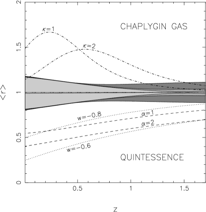
Figure 6: Variation of $<r(z)>$ with $z$ for the cosmological constant model. Solid line shows best-fit $<r(z)>$ averaged over all realizations calculated with the polynomial fit to dark energy, Eq (35), for the prior $\Omega_{m}=0.3$ exactly. The triple-dot-dashed line represents the exact value of $<r>=1$ for the cosmological constant model. Shaded regions represent the $1\sigma$ confidence levels for $<r(z)>$. The dark grey outer contour is for the Gaussian prior $\Omega_{m}=0.3\pm\sigma_{\Omega_{m}}$ with $\sigma_{\Omega_{m}}=0.05$, the grey contour in the middle uses the Gaussian prior $\sigma_{\Omega_{m}}=0.015$, and the light grey contour uses $\Omega_{m}=0.3$ exactly. The dotted, dashed and dot-dashed lines represent the exact values of $r(z)$ for different constant $w$ quiessence models, for kinessence models with the tracker potential $V(\phi)=V_{0}/\phi^{\alpha}$ for different values of $\alpha$, and for Chaplygin gas models with different $\kappa$ respectively. We see that all the model values plotted lie outside the $1\sigma$ confidence level even for the most conservative prior of $\sigma_{\Omega_{m}}=0.05$ at redshifts $\lower 3.48746pt\hbox{ $\buildrel>\over{\sim}$}~{}0.3$.

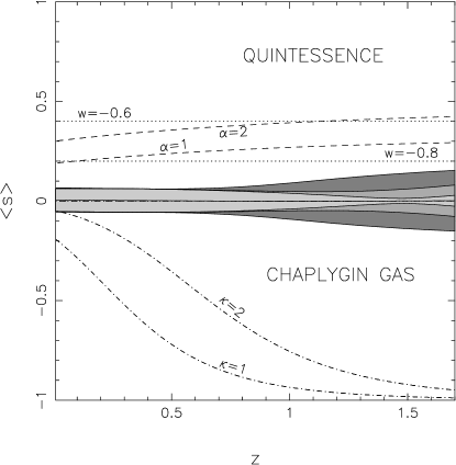
Figure 7: Variation of $<s(z)>$ with $z$ for the cosmological constant model. Solid line shows best-fit $<s(z)>$ averaged over all realizations calculated with the polynomial fit to dark energy, Eq (35), for the prior $\Omega_{m}=0.3$ exactly. The triple-dot-dashed line represents the exact value of $<s>=0$ for the cosmological constant model. Shaded regions represent the $1\sigma$ confidence levels for $<s(z)>$. The dark grey outer contour is for the Gaussian prior $\Omega_{m}=0.3\pm\sigma_{\Omega_{m}}$ with $\sigma_{\Omega_{m}}=0.05$, the grey contour in the middle uses the Gaussian prior $\sigma_{\Omega_{m}}=0.015$, and the light grey contour uses $\Omega_{m}=0.3$ exactly. The dotted, dashed and dot-dashed lines represent the exact values of $s(z)$ for different constant $w$ quiessence models, for kinessence models with the tracker potential $V(\phi)=V_{0}/\phi^{\alpha}$ for different values of $\alpha$, and for Chaplygin gas models with different $\kappa$ respectively. We see that all the model values plotted lie outside the $1\sigma$ confidence level even for the most conservative prior of $\sigma_{\Omega_{m}}=0.05$.

Figure 4 shows the $99.73\%$ confidence level in $\{\bar{s},\bar{r}\}$ (left panel) and $\{\bar{s},\bar{q}\}$ (right panel) for the fiducial LCDM model with $\Omega_{m}=0.3$, $\Omega_{\Lambda}=0.7$. For comparison we also show values of $\bar{r},\bar{s},\bar{q}$ for quiessence, kinessence and Chaplygin gas models. From this figure we see that the statefinders can easily distinguish LCDM from: (i) quiessence with $w\lower 3.87495pt\hbox{ $\buildrel>\over{\sim}$}~{}-0.9$ (ii) the Chaplygin gas with $\kappa\lower 3.87495pt\hbox{ $\buildrel<\over{\sim}$}~{}15$ (iii) the quintessence potential $V(\phi)\propto\phi^{-\alpha},\alpha\lower 3.87495pt\hbox{ $\buildrel>\over{\sim}$}~{}1$ and (iv) the DDG braneworld models discussed in Deffayet et al. (2002).

The above analysis assumed that the value of $\Omega_{m}$ is known exactly. However in practice it will be some time before $\Omega_{m}$ is known to 100% accuracy and it is only natural to expect some amount of uncertainty in the observational value of this important physical parameter. We incorporate this uncertainty by marginalizing over the value of $\Omega_{m}$. Two priors will be incorporated into our analysis, the weak Gaussian prior: $\Omega_{m}=0.3\pm 0.05$ and the stronger Gaussian prior: $\Omega_{m}=0.3\pm 0.015$.

Figures  5 (a-d), show the confidence levels in the statefinder pairs $\{\bar{s},\bar{r}\}$, $\{\bar{s},\bar{q}\}$, $\{s_{0},r_{0}\}$ and $\{s_{0},q_{0}\}$ respectively. For purposes of discrimination we also show the values of the $r,s,q$ for quiessence, kinessence, Chaplygin gas and braneworld models. Figure 5(a) shows that the diagnostic $\{\bar{s},\bar{r}\}$ permits the LCDM model to be distinguished from quiessence models with $w\lower 3.87495pt\hbox{ $\buildrel>\over{\sim}$}~{}-0.8$, quintessence models with $\alpha\geq 1$, Chaplygin gas models with $\kappa\lower 3.87495pt\hbox{ $\buildrel<\over{\sim}$}~{}6$ and braneworld models at the $99.73\%$ confidence level and after applying the strong Gaussian prior of $\Omega_{m}=0.3\pm 0.015$. The discriminatory power of the statefinder clearly worsens for the weaker prior $\Omega_{m}=0.3\pm 0.05$.

The situation can be dramatically improved if, instead of working with $\{\bar{s},\bar{r}\}$ we use the diagnostic $\{\bar{s},\bar{q}\}$ (see figure 5 (b)). We find in this case that the fiducial LCDM model can be distinguished from quiessence with $w\lower 3.87495pt\hbox{ $\buildrel>\over{\sim}$}~{}-0.85$ and the braneworld model at the $99.73\%$ confidence level even for the weak prior $\Omega_{m}=0.3\pm 0.05$. In Figures 5(c) & (d) we plot the confidence levels for current values of the pair $\{s_{0},r_{0}\}$ and $\{s_{0},q_{0}\}$. A few important points need to be noted here:

$\begin{array}[]{c@{\hspace{0.4in}}c}\lx@intercol\mbox{}\hfil\lx@intercol&\lx@intercol\mbox{}\hfil\lx@intercol\\[0.0pt] \epsfbox{h_exp_rs_comp1.epsi}\hfil\hskip 28.90755pt&\epsfbox{h_exp_rs_comp2.epsi}\\ \mbox{\bf(a)}\hfil\hskip 28.90755pt&\mbox{\bf(b)}\end{array}$

Figure 8: $3\sigma$ confidence levels in the parameter space $\bar{r},\bar{s}$ are shown for the cosmological constant model and the $\alpha=1$ tracker model using the polynomial fit to dark energy, Eq (35). The solid stars represent the model value of the parameter pair for the cosmological constant model and the $\alpha=1$ tracker kinessence models. The dashed line above the LCDM point represents the quiessence models, and that below the LCDM point represents different Chaplygin gas models. The solid triangles represent model values for constant $w$ quiessence models, and the solid hexagons represent Chaplygin gas models with different values of $\kappa$. Only those Chaplygin gas models with $\kappa\geq\Omega_{m}/(1-\Omega_{m})$ are allowed. For all the dark energy models, $\Omega_{m}=0.3$ is used. The ellipses represent the $3\sigma$ confidence levels in the $\bar{r}-\bar{s}$ space for the exact prior $\Omega_{m}=0.3$. In (a), the dark grey contour in solid outline represents the confidence level for the cosmological constant fiducial model obtained when $r,s$ are averaged over the redshift range $z=0$ to $z=1.7$. The light grey contour with dotted outline is the confidence level for the $\alpha=1$ tracker kinessence model obtained when the averaging is over the entire redshift range. In (b), we show confidence levels for the cosmological constant model (dark grey contour) and for the $\alpha=1$ tracker model (light grey contour) with the averaging done from $z=1$ to $z=1.7$. Remarkably, using the statefinders $\{\bar{r},\bar{s}\}$ one can rule out quintessence models with $w\lower 3.48746pt\hbox{ $\buildrel>\over{\sim}$}~{}-0.95$ and Chaplygin gas models with $\kappa\lower 3.48746pt\hbox{ $\buildrel<\over{\sim}$}~{}24$ at $3\sigma$ if only very high redshift SNe belonging to the redshift interval $1\leq z\leq 1.7$ are considered. The reason for this is that both $r(z)$ and $s(z)$ are determined to increasing accuracy at $z\lower 3.48746pt\hbox{ $\buildrel>\over{\sim}$}~{}1$. Indeed, a ‘sweet spot’ at $z_{s}\simeq 1.4$ ensures that both $r(z_{s})$ & $s(z_{s})$ are known with great accuracy at that point – see figures ( 6) & ( 7).

(i) the semi-major axis of the confidence ellipse for $\{s,q\}$ is tilted away from the dashed curve representing constant $w$ models (quiessence). This enables the second statefinder pair $\{s,q\}$ to be somewhat better at discriminating between LCDM and quintessence models than $\{r,s\}$. For instance, the current value $\{s_{0},q_{0}\}$ can discriminate the cosmological constant model from quiessence models having $w\lower 3.87495pt\hbox{ $\buildrel>\over{\sim}$}~{}-0.9$, kinessence models with $\alpha\geq 1$, Chaplygin gas models with $\kappa\lower 3.87495pt\hbox{ $\buildrel<\over{\sim}$}~{}2$, and the braneworld model even after applying the weak Gaussian prior $\Omega_{m}=0.3\pm 0.05$.

(ii) For Chaplygin gas models averaging over redshift considerably enhances the discriminatory prowess of both $\{\bar{s},\bar{r}\}$ and $\{\bar{s},\bar{q}\}$.

(iii) From figure (5d) we find that marginalization over $\Omega_{m}$ has only a small effect on the diagnostic $\{s_{0},q_{0}\}$ which contributes to making this statefinder pair a much better discriminator of dark energy than $\{r_{0},s_{0}\}$ if the value of $\Omega_{m}$ is uncertain.

Our results shown in figures  4 & 5 clearly demonstrate that both $\{r,s\}$ as well as $\{s,q\}$ are excellent diagnostics of dark energy with the latter being somewhat more sensitive than the former.

We now proceed to examine the information content in the cosmological parameters when examined individually. In Figure 6, we plot the variation of the ensemble averaged value $\langle r(z)\rangle$ with redshift. The $1\sigma$ error bounds are shown for two different priors on $\Omega_{m}$ and for the case when the value of $\Omega_{m}$ is known exactly. This figure shows that $r(z)$ is a good diagnostic of dark energy and allows us to discriminate (at the $68.3\%$ CL) between different dark energy models and LCDM. Discrimination improves at higher redshifts ($z\lower 3.87495pt\hbox{ $\buildrel>\over{\sim}$}~{}0.8$) especially if the uncertainty in the value of $\Omega_{m}$ is small. The sweet spot for this parameter, ${\it i.e.~{}}$ the point at which $r(z)$ is most accurately determined, is at $z\sim 1.4$. (For earlier work on the sweet spot see Weller & Albrecht, 2002; Huterer & Turner, 1999; Huterer & Starkman, 2002).

Figure 7 shows the variation of the ensemble averaged value of the second statefinder $\langle s(z)\rangle$ with redshift. Again $1\sigma$ errors for the two priors $\Omega_{m}=0.3\pm 0.05$, $\Omega_{m}=0.3\pm 0.015$ and when the value of $\Omega_{m}$ is known exactly ($\Omega_{m}=0.3$) are shown. We see that $s(z)$ is determined even more accurately than $r(z)$, and therefore can serve as a better diagnostic of dark energy. For the strong Gaussian prior $\Omega_{m}=0.3\pm 0.015$, (or when $\Omega_{m}$ is known exactly) the value of $s$ is very well determined even at higher redshifts, its sweet spot being at $z\sim 1.4$. For the weak prior $\Omega_{m}=0.3\pm 0.05$, $s$ is not so well determined at high redshifts, but it is still accurate enough to distinguish between rival models of dark energy. Two points are of interest here. Firstly, $r$ and $s$ are both much more accurately determined at higher redshifts if the value of $\Omega_{m}$ is accurately known. This explains why the parameters $\{\bar{r},\bar{s}\}$ perform better as discriminators than $\{r_{0},s_{0}\}$. Secondly, the sweet spot for both these parameters appears at $z\sim 1.4$, only if the value of $\Omega_{m}$ is accurately known. Upon marginalizing over $\Omega_{m}$ the sweet spot disappears both in the case of $r(z)$ as well as in the case of $s(z)$. Another point worth mentioning is that Chaplygin gas models are much easier to rule out at high $z$ than at low $z$, using either $r(z)$ or $s(z)$. As an illustration, neither $r_{0}$ nor $s_{0}$ can distinguish a $\kappa=2$ Chaplygin gas model from LCDM (with identical $\Omega_{m}$) at the $1\sigma$ level. However the averaged-over-redshift statefinders $\bar{r},\bar{s}$ can do so quite easily even at the $3\sigma$ level, as demonstrated in figures 4 and 5.

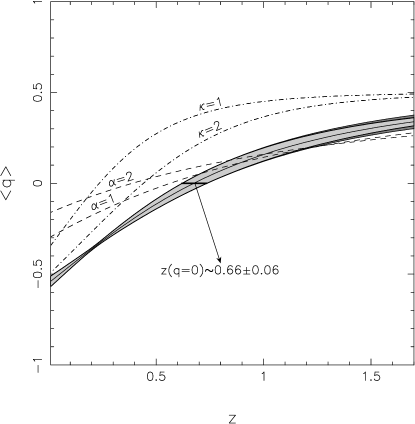
Figure 9: Variation of $<q(z)>$ with $z$ for the cosmological constant model. Solid line shows best-fit $<q(z)>$ averaged over all realizations calculated with the polynomial fit to dark energy, Eq (35), for the prior $\Omega_{m}=0.3$ exactly. Shaded regions represent the $1\sigma$ confidence levels for $<q>$. We find here that the use of exact $\Omega_{m}=0.3$ and the Gaussian prior $\Omega_{m}=0.3\pm\sigma_{\Omega_{m}}$ with $\sigma_{\Omega_{m}}=0.015$ gives us almost the same bounds, represented by the light grey contour, the dark grey outer contour uses the Gaussian prior $\sigma_{\Omega_{m}}=0.05$. The dotted, dashed and dot-dashed lines represent the model values of $<q>$ for different constant $w$ quiessence models, for kinessence models with the tracker potential $V(\phi)=V_{0}/\phi^{\alpha}$ for different values of $\alpha$, and for Chaplygin gas models with different $\kappa$ respectively. The horizontal thick line represents the accuracy with which the acceleration epoch is determined in this fit. This figure demonstrates that $q$ can be used as a discriminator between dark energy models at low redshifts$\lower 3.48746pt\hbox{ $\buildrel<\over{\sim}$}~{}0.5$. Indeed the location of a sweet spot at $z_{s}\simeq 0.2$ demonstrates that the value of $q(z_{s})$ is known to remarkably good accuracy !

$\begin{array}[]{c@{\hspace{0.4in}}c}\lx@intercol\mbox{}\hfil\lx@intercol&\lx@intercol\mbox{}\hfil\lx@intercol\\[0.0pt] \epsfbox{h_exp_qs_comp1.epsi}\hfil\hskip 28.90755pt&\epsfbox{h_exp_qs_comp2.epsi}\\ \mbox{\bf(a)}\hfil\hskip 28.90755pt&\mbox{\bf(b)}\end{array}$

Figure 10: $3\sigma$ confidence levels in the parameter space $\bar{q},\bar{s}$ are shown for the cosmological constant model and the $\alpha=1$ tracker model using the polynomial fit to dark energy, Eq (35). The solid stars represent the model value of the parameter pair for the cosmological constant model and the $\alpha=1$ tracker kinessence models. The dashed line above the LCDM point represents the quiessence models, and that below the LCDM point represents different Chaplygin gas models. The solid triangles represent model values for constant $w$ quiessence models, and the solid hexagons represent Chaplygin gas models with different values of $\kappa$. Only those Chaplygin gas models with $\kappa\geq\Omega_{m}/(1-\Omega_{m})$ are allowed. For all the dark energy models, $\Omega_{m}=0.3$ is used. The ellipses represent the $3\sigma$ confidence levels in the $\bar{q}-\bar{s}$ space for the exact prior $\Omega_{m}=0.3$. In (a), the dark grey contour in solid outline represents the confidence level for the cosmological constant fiducial model obtained when $q,s$ are averaged in the redshift range $z=0$ to $z=1.7$. The light grey contour with dotted outline is the confidence level for the $\alpha=1$ tracker kinessence model obtained when the averaging is over the entire redshift range. In (b), we show confidence levels for the cosmological constant model (dark grey contour) and for the $\alpha=1$ tracker model (light grey contour) with the averaging done from $z=0$ to $z=0.4$ for $q$ and from $z=1$ to $z=1.7$ for $s$. The reason for choosing these ranges is that $q$ is extremely well-determined at low redshifts, with a sweet spot at $z_{s}\simeq 0.25$, and $s$ is accurately determined at high redshifts with a sweet spot at $z_{s}\simeq 1.4$ – see figures ( 9) & ( 7). Using the second statefinder pair $\{\bar{q},\bar{s}\}$ one can rule out quintessence models with $w\lower 3.48746pt\hbox{ $\buildrel>\over{\sim}$}~{}-0.95$ and Chaplygin gas models with $\kappa\lower 3.48746pt\hbox{ $\buildrel<\over{\sim}$}~{}25$ at $3\sigma$ if only very high redshift SNe belonging to the redshift interval $1\leq z\leq 1.7$ are considered for $s$ and low redshift SNe in the interval $0\leq z\leq 0.4$ are considered for $q$.

Figure 8 shows how sweet spot information can be used to improve the statefinders as a diagnostic tool. For both $r$ and $s$ the sweet spot appears at high redshifts. Therefore, one expects that the discriminatory prowess of the statefinders will improve considerably if only data at $z\geq 1$ is considered. This is indeed the case. Figure 8 shows $3\sigma$ confidence levels in $\{\bar{r},\bar{s}\}$ for two cases: (a) the statefinder pair is averaged over the full redshift range $0\leq z\leq 1.7$, (b) the statefinder pair is averaged over the high redshift range $1\leq z\leq 1.7$; $\Omega_{m}=0.3$ for both cases. The dark grey ellipses represent the confidence level for the LCDM model, and the light grey ellipses represent the confidence level for the $\alpha=1$ kinessence model. We see that there is a dramatic improvement in the determination of the statefinder pair in figure 8(b) where the statefinders have been averaged only for $z\geq 1$. From figure 8 (a) we see that $\{\bar{r},\bar{s}\}$ can discriminate between LCDM and quiessence models with $w\lower 3.87495pt\hbox{ $\buildrel>\over{\sim}$}~{}-0.90$ and Chaplygin gas models with $\kappa\lower 3.87495pt\hbox{ $\buildrel<\over{\sim}$}~{}15$, whereas 8(b) shows that $\{\bar{r},\bar{s}\}$ can discriminate between LCDM and quiessence models with $w\lower 3.87495pt\hbox{ $\buildrel>\over{\sim}$}~{}-0.95$ and Chaplygin gas models with $\kappa\lower 3.87495pt\hbox{ $\buildrel<\over{\sim}$}~{}24$ ! We therefore conclude that high redshift supernovae can play a crucial role in constraining properties of dark energy and our results support the views expressed in Linder & Huterer (2003). We must however note that in order to use sweet spot information optimally the value of $\Omega_{m}$ must be known to very high accuracy. Indeed, for the Gaussian prior of $\Omega_{m}=0.3\pm 0.05$, a consideration of only high redshift supernovae does not lead to any improvement in the results. This is because, as seen from Figures 6 & 7, after marginalization over $\Omega_{m}$, the sweet spot for both $r(z)$ and $s(z)$ disappears. The second point to note is that the angle of inclination of the semi-major axis of the ellipse to the $w=$ constant curve (quiessence) appears to depend upon the redshift range over which the statefinder pair is being averaged.

Figure 9 shows the variation of the mean deceleration parameter $q(z)$ with redshift. We see that $q(z)$ is very well determined over the entire range $0\leq z\leq 1.7$. This justifies our choice of $\{s,q\}$ as the second statefinder pair. Indeed, the behaviour of $r(z)$ and $s(z)$ on the one hand and $q(z)$ on the other, is in some ways complementary. While both $r(z)$ and $s(z)$ are determined to increasing accuracy at higher redshifts, the deceleration parameter is very well determined at lower redshifts and the sweet spot for this parameter appears at the redshift $z_{s}\simeq 0.25$. It is interesting that, in sharp contrast to what was earlier observed for $r$ and $s$, the sweet spot in $q(z)$ persists even after we marginalize over $\Omega_{m}$ ! From figure 9 we can also determine the value of the acceleration epoch (the redshift at which the universe began accelerating). We find that the acceleration epoch is determined quite accurately: $z(q=0)=0.66\pm 0.06$.

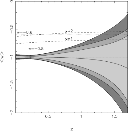
Figure 11: Variation of $<w(z)>$ with $z$ for the cosmological constant model. Solid line shows best-fit $<w(z)>$ averaged over all realizations calculated with the polynomial fit to dark energy, Eq (35), for the prior $\Omega_{m}=0.3$ exactly. The dot-dashed line represents the exact value of $<w>=-1$ for the cosmological constant model. Shaded regions represent the $1\sigma$ confidence levels for $<w>$. The dark grey outer contour is for the Gaussian prior $\Omega_{m}=0.3\pm\sigma_{\Omega_{m}}$ with $\sigma_{\Omega_{m}}=0.05$, the grey contour in the middle uses the Gaussian prior $\sigma_{\Omega_{m}}=0.015$, and the light grey contour uses $\Omega_{m}=0.3$ exactly. The dotted and dashed lines represent the model values of $<w>$ for different constant $w$ quiessence models and for kinessence models with the tracker potential $V(\phi)=V_{0}/\phi^{\alpha}$ for different values of $\alpha$ respectively. We see that $w$ can distinguish between the cosmological constant model and other dark energy models only at $z\lower 3.48746pt\hbox{ $\buildrel<\over{\sim}$}~{}1$.

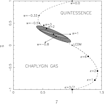
Figure 12: $3\sigma$ confidence levels in the parameter space $\bar{r},\bar{s}$ are shown for the kinessence model with tracker potential $V=V_{0}/\phi^{\alpha}$ for $\alpha=1$, for the polynomial fit to dark energy, Eq (35). The solid star represents the model value of the parameter pair for the cosmological constant model. The dashed line above the LCDM point represents the quiessence models, and that below the LCDM point represents different Chaplygin gas models. The solid rhombi represent tracker kinessence models with different $\alpha$, the solid triangles represent the constant $w$ quiessence models, and the solid hexagons represent Chaplygin gas models with different values of $\kappa$. Only those Chaplygin gas models with $\kappa\geq\Omega_{m}/(1-\Omega_{m})$ are allowed. For all the dark energy models, $\Omega_{m}=0.3$ is used. The square represents the best-fit for the $\alpha=1$ fiducial model. The shaded ellipses represent the $3\sigma$ confidence levels in the $\bar{r}-\bar{s}$ space. The dark grey outer contour is for the Gaussian prior with $\sigma_{\Omega_{m}}=0.05$, the grey contour in the middle uses the Gaussian prior $\sigma_{\Omega_{m}}=0.015$, and the light grey contour uses $\Omega_{m}=0.3$ exactly.

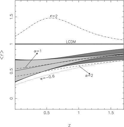
Figure 13: Variation of $<r(z)>$ with $z$ for the kinessence model with the tracker potential $V(\phi)=V_{0}/\phi^{\alpha}$ for $\alpha=1$. Solid line shows best-fit $<r(z)>$ averaged over all realizations calculated with the polynomial fit to dark energy, Eq (35), for the prior $\Omega_{m}=0.3$ exactly. Shaded regions represent the $1\sigma$ confidence levels for $<r>$. The dark grey outer contour is for the Gaussian prior $\Omega_{m}=0.3\pm\sigma_{\Omega_{m}}$ with $\sigma_{\Omega_{m}}=0.05$, the grey contour in the middle uses the Gaussian prior $\sigma_{\Omega_{m}}=0.015$, and the light grey contour uses $\Omega_{m}=0.3$ exactly. The dotted, dashed and dot-dashed lines represent the model values of $<r>$ for different constant $w$ quiessence models, for tracker kinessence models for different values of $\alpha$, and for Chaplygin gas models with different $\kappa$ respectively. The thick solid line represents LCDM.

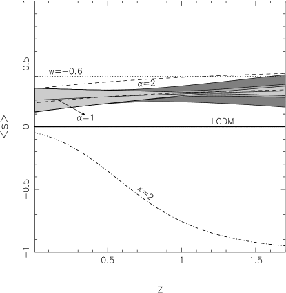
Figure 14: Variation of $<s(z)>$ with $z$ for the kinessence model with the tracker potential $V(\phi)=V_{0}/\phi^{\alpha}$ for $\alpha=1$. Solid line shows best-fit $<s(z)>$ averaged over all realizations calculated with the polynomial fit to dark energy, Eq (35), for the prior $\Omega_{m}=0.3$ exactly. Shaded regions represent the $1\sigma$ confidence levels for $<s>$. The dark grey outer contour is for the Gaussian prior $\Omega_{m}=0.3\pm\sigma_{\Omega_{m}}$ with $\sigma_{\Omega_{m}}=0.05$, the grey contour in the middle uses the Gaussian prior $\sigma_{\Omega_{m}}=0.015$, and the light grey contour uses $\Omega_{m}=0.3$ exactly. The dotted, dashed and dot-dashed lines represent the model values of $<s>$ for different constant $w$ quiessence models, for tracker kinessence models for different values of $\alpha$, and for Chaplygin gas models with different $\kappa$ respectively. The thick solid line represents LCDM.

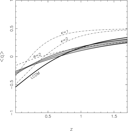
Figure 15: Variation of $<q(z)>$ with $z$ for the kinessence model with the tracker potential $V(\phi)=V_{0}/\phi^{\alpha}$ for $\alpha=1$. Solid line shows best-fit $<q(z)>$ averaged over all realizations calculated with the polynomial fit to dark energy, Eq (35), for the prior $\Omega_{m}=0.3$ exactly. Shaded regions represent the $1\sigma$ confidence levels for $<q>$. We find here that the use of exact $\Omega_{m}=0.3$ and the Gaussian prior $\Omega_{m}=0.3\pm\sigma_{\Omega_{m}}$ with $\sigma_{\Omega_{m}}=0.015$ gives us almost the same bounds, represented by the light grey contour, the dark grey outer contour uses the Gaussian prior $\sigma_{\Omega_{m}}=0.05$. The dashed and dot-dashed lines represent the model values of $<s>$ for tracker kinessence models for different values of $\alpha$, and for Chaplygin gas models with different $\kappa$ respectively. The thick solid line represents LCDM.

Figure 16: $3\sigma$ confidence levels in the parameter space $\bar{r},\bar{s}$ are shown for the cosmological constant model using the polynomial fit to luminosity distance, Eq (39). The solid star represents the model value of the parameter pair for the cosmological constant model. The dashed line above the LCDM point represents the quiessence models, and that below the LCDM point represents different Chaplygin gas models. The solid rhombi represent tracker kinessence models with different $\alpha$, the solid triangles represent model values for constant $w$ quiessence models, and the solid hexagons represent Chaplygin gas models with different values of $\kappa$. Only those Chaplygin gas models with $\kappa\geq\Omega_{m}/(1-\Omega_{m})$ are allowed. For all the dark energy models, $\Omega_{m}=0.3$ is used. The best-fit point for the reconstruction is represented by the solid square. The ellipses represent the $1\sigma$, $2\sigma$, $3\sigma$ confidence levels in the $\bar{r}-\bar{s}$ space.

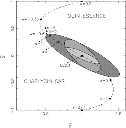
Figure 17: $3\sigma$ confidence levels in the parameter space $\bar{r},\bar{s}$ are shown for the cosmological constant model using the polynomial fit to equation of state, Eq (41). The solid star represents the model value of the parameter pair for the cosmological constant model. The dashed line above the LCDM point represents the quiessence models, and that below the LCDM point represents different Chaplygin gas models. The solid rhombi represent tracker kinessence models with different $\alpha$, the solid triangles represent model values for constant $w$ quiessence models, and the solid hexagons represent Chaplygin gas models with different values of $\kappa$. Only those Chaplygin gas models with $\kappa\geq\Omega_{m}/(1-\Omega_{m})$ are allowed. For all the dark energy models, $\Omega_{m}=0.3$ is used. The best-fit point lies on the LCDM point for this reconstruction. The shaded ellipses represent the $3\sigma$ confidence levels in the $\bar{r}-\bar{s}$ space. The dark grey outer contour is for the Gaussian prior $\Omega_{m}=0.3\pm\sigma_{\Omega_{m}}$ with $\sigma_{\Omega_{m}}=0.05$, the grey contour in the middle uses the Gaussian prior $\sigma_{\Omega_{m}}=0.015$, and the light grey contour uses $\Omega_{m}=0.3$ exactly.

Figure 10 shows maximum likelihood contours for the pair $\{\bar{s},\bar{q}\}$ where $\bar{q}$ has been averaged over the redshift interval $0<z\leq 0.4$ while $\bar{s}$ has been averaged over $1\leq z\leq 1.7$. This figure clearly demonstrates that $\{\bar{s},\bar{q}\}$ is an excellent diagnostic of dark energy since it can distinguish LCDM from quiessence models with $w\geq-0.95$ on the one hand and from Chaplygin gas models with $\kappa\leq 25$ on the other (both at the $99.73\%$ CL). Figures 8 and 10 show that the ability of the averaged statefinder pairs $\{\bar{s},\bar{r}\}$ and $\{\bar{s},\bar{q}\}$ to discriminate between dark energy models is comparable if the value of $\Omega_{m}$ is known exactly. (As demonstrated earlier in figure (5), $\{s,q\}$ is a more sensitive diagnostic than $\{r,s\}$ if we marginalize over $\Omega_{m}$.)

Figure 11 shows how the equation of state $w(z)$ varies with redshift. We see that, although the equation of state is determined remarkably well at small redshifts, cosmological reconstruction of $w(z)$ steadily worsens with $z$ and deteriorates rapidly beyond $z\simeq 1$. With the most conservative prior $\Omega_{m}=0.3\pm 0.05$, the ansatz (35) can distinguish between the cosmological constant model and the quiessence model with $w=-0.96$ at the $3\sigma$ level provided we restrict ourselves to low redshifts $z\lower 3.87495pt\hbox{ $\buildrel<\over{\sim}$}~{}0.4$. For higher redshifts, the LCDM model cannot be distinguished from the $w=-0.8$ model beyond $z\simeq 1.1$ (after marginalizing over $\Omega_{m}$ with the prior $\Omega_{m}=0.3\pm 0.05$). In the ideal case when $\Omega_{m}=0.3$ exactly, LCDM and the $w=-0.8$ model can be distinguished up to $z\sim 1.3$ but not beyond. (In this case the best-fit $w(z)$ is biased beyond $z\simeq 0.7$ and takes on a lower value than the fiducial $w=-1$.) Somewhat surprisingly, although $w(z)$ and $q(z)$ are related through (6) and therefore carry essentially the same information, even a cursory examination of figures 9 and 11 reveals that the ansatz (35) does not reconstruct $w(z)$ to the same accuracy as it reconstructs $q(z)$. However, like $q(z)$, $w(z)$ is reasonably well determined at low redshifts, having a sweet spot at $z\sim 0.25$. The sweet spot persists when we marginalize over $\Omega_{m}$ using the Gaussian prior $\Omega_{m}=0.3\pm 0.015$ but disappears when the uncertainty in $\Omega_{m}$ is increased using the prior $\Omega_{m}=0.3\pm 0.05$.

5.2 Cosmological reconstruction for a tracker model

We now briefly examine the accuracy of the statefinder pair and the ansatz (35) in determining the statefinder pair for a fiducial model other than LCDM. We know that the ansatz returns exact values for the cosmological constant $w=-1$ as well as for quiessence having the constant equation of state $w=-2/3$ and $w=-1/3$ (see figure 3). It is therefore important to study the accuracy of the statefinder in reconstructing the properties of dark energy in models in which both the dark energy density as well as the equation of state vary with time and for which the ansatz (35) is approximate. For this purpose we shall work with a fiducial dark energy model which evolves under the influence of the tracker potential $V=V_{0}/\phi$ and use the ansatz (35) in tandem with the statefinders (3) to reconstruct the properties of dark energy.

Figure 12 shows our results in terms of $3\sigma$ confidence levels in $\{\bar{r},\bar{s}\}$. We find that, if the value of $\Omega_{m}$ is known to reasonable accuracy ($\Omega_{m}=0.3\pm 0.015$) then the averaged statefinder pair $\{\bar{r},\bar{s}\}$ is able to distinguish the model $V=V_{0}/\phi$ from the model $V=V_{0}/\phi^{2}$ at the $3\sigma$ level. As expected, a large uncertainty in the current value of the matter density reduces the efficiency of this diagnostic and the two models $V=V_{0}/\phi$ and $V=V_{0}/\phi^{2}$ cannot be clearly distinguished if the uncertainty in $\Omega_{m}$ is increased to $\Omega_{m}=0.3\pm 0.05$.

Figures 13 & 14 show the performance of the ensemble averaged statefinders $\langle r(z)\rangle$ and $\langle s(z)\rangle$. As in the earlier case when our fiducial model was assumed to be LCDM, we find that the errors in $r(z)$ and $s(z)$ are small. However a slight bias in the determination of the statefinders exists at low redshifts so that for $z\lower 3.87495pt\hbox{ $\buildrel<\over{\sim}$}~{}0.4$ the value of the best fit $\langle r\rangle$ ($\langle s\rangle$) is larger (smaller) than the exact fiducial value. Averaging over the entire redshift range can significantly reduce this bias and we conclude that the ansatz (35) works well even for those dark energy models for which it does not return exact values. One should also note the reappearance of the sweet spot for the statefinders $r$ & $s$ in the figures 13 & 14. For the statefinder $r(z)$ the sweet spot appears at $z\simeq 1.6$, while for $s(z)$ the sweet spot is at $z\simeq 1.2$. As in the case of the LCDM model, one can try and constrain the properties of dark energy further by evaluating the averaged statefinders using SNe data only from $z\geq 1$. Our results shown in figure 8 demonstrate that the confidence ellipse for $\{\bar{s},\bar{r}\}$ becomes much smaller when the averaging is done over the redshift range $1\leq z\leq 1.7$ than when the averaging is over the entire redshift range.

The performance of the deceleration parameter $\langle q(z)\rangle$ for this quintessence model is shown in the figure 15. We see that the deceleration parameter is very accurately determined. The sweet spot for the deceleration parameter occurs at lower redshifts, at $z\simeq 0.2$, and by combining higher redshift data in determining $\bar{s}$ with lower redshift data for determining $\bar{q}$ we can significantly improve the errors on the second statefinder pair $\{s,q\}$, as demonstrated in figure 10. As was the case for the LCDM model, the sweet spot gradually disappears if we incorporate the prevailing uncertainty in the value of the matter density by marginalizing over large values of $\Omega_{m}$.

5.3 Cosmological reconstruction using other fitting functions

For comparison, we also carry out the reconstruction exercise using two of the fitting functions described in section 4.1. In figure 16 we show the results for $\{\bar{r},\bar{s}\}$ using the polynomial fit to the luminosity distance (39) with $N=5$. In this case, because of the nature of the ansatz, it is not possible to place any priors on $\Omega_{m}$. We find that this ansatz does not perform well for the statefinder pair. Firstly, it does not determine $\bar{r},\bar{s}$ with the accuracy seen in the case of the polynomial fit to dark energy. Secondly, the best-fit value for $\{\bar{r},\bar{s}\}$ is biased with respect to the fiducial LCDM value. Additionally, the errors on both $r$ and $s$ are unacceptably large due to which one cannot distinguish between the cosmological constant model and kinessence models with $\alpha<6$, quiessence models with $w\lower 3.87495pt\hbox{ $\buildrel<\over{\sim}$}~{}-0.4$, and Chaplygin gas models with $\kappa\lower 3.87495pt\hbox{ $\buildrel>\over{\sim}$}~{}2$ at the $3\sigma$ confidence level. Even at $1\sigma$ ($68.3\%$ CL), one can only discriminate LCDM from kinessence models with $\alpha\geq 3$, quiessence models with $w\lower 3.87495pt\hbox{ $\buildrel>\over{\sim}$}~{}-0.6$, and Chaplygin gas models with $\kappa\lower 3.87495pt\hbox{ $\buildrel<\over{\sim}$}~{}3$. We therefore conclude that the polynomial fit to the luminosity distance (39) is not very useful for the reconstruction of the statefinders.

We also carry out a similar reconstruction exercise using the polynomial fit to the equation of state (41) with $N=1$. This ansatz can accommodate priors on $\Omega_{m}$ and we expect it to perform better than the polynomial fit to the luminosity distance. Indeed, figure 17 clearly demonstrates that a two parameter Taylor expansion in the equation of state is better than a five parameter expansion in the luminosity distance (Our results in this context support the earlier observations of Weller & Albrecht, 2002). From figure 17 we find that the ansatz (41) can distinguish the cosmological constant model from quiessence models with $w\lower 3.87495pt\hbox{ $\buildrel>\over{\sim}$}~{}-0.6$, kinessence models with $\alpha\geq 3$, and Chaplygin gas models with $\kappa\lower 3.87495pt\hbox{ $\buildrel<\over{\sim}$}~{}3$ at the $99.73\%$ confidence limit after we have marginalized over $\Omega_{m}$ with a Gaussian prior of $\Omega_{m}=0.3\pm 0.05$. However a comparison of figure 17 with figure 5 shows that the equation of state expansion (41) is not quite as accurate as the polynomial fit to dark energy (35) in reconstructing the statefinder pair $\{\bar{r},\bar{s}\}$. We therefore conclude that the statefinders can be reconstructed using several complementary methods. The polynomial fit for dark energy (35), by providing a good reconstruction of the parameters $\bar{r},\bar{s},\bar{q}$, can successfully be used for the model independent reconstruction of dark energy.

6 Conclusions and discussion

This paper contains an in depth study of properties of the statefinder diagnostic introduced in Sahni et al.  (2003). The statefinder pairs $\{r,s\}$ and $\{s,q\}$ have the potential to successfully discriminate between a wide variety of dark energy models including the cosmological constant, quintessence, the Chaplygin gas and braneworld models. The statefinders play a particularly important role in the case of modified gravity theories such as string/M-theory inspired scalar-tensor models and braneworld models of dark energy, for which the equation of state is not a fundamental physical entity and therefore does not provide us with an adequate description of the accelerating universe. Our results, summarized in figures 1 and 2, show that the statefinders $r$, $s$ considerably extend and supplement traditional measures of cosmological dynamics such as the deceleration parameter $q$. To give a concrete example of how this can happen consider two (or more) cosmological dark energy models which have identical (hence degenerate) values of $q_{0}$. Although such models will have the same current value of ${\ddot{a}}/a$, the value of the third derivative $\stackrel{{\scriptstyle...}}{{a}}$ (hence $r$ & $s$) will in general be different in both models. The statefinder pairs $\{r,q\}$ and $\{s,q\}$ therefore provide us with a ‘phase-space’ picture of dark energy which distinguishes dynamical dark energy models both from each other as well as from the cosmological constant and helps break cosmological degeneracies present in rival models of dark energy. The statefinder $s$ is remarkably sensitive to the total pressure of all forms of matter and radiation in the universe. As a result $s$ remains sensitive to the presence of dark energy even at moderately high redshifts $z\sim 10$, when the universe is matter dominated.

Forthcoming space-based missions such as SNAP are expected to greatly increase and improve the current Type Ia supernova inventory. Anticipating this development we have carried out a maximum likelihood analysis which combines the statefinder diagnostic with realistic expectations from the SNAP experiment. Our results, summarized in figures 4 - 10, show that both $\{r,s\}$ as well as $\{s,q\}$ are excellent diagnostics of dark energy. If the value of $\Omega_{m}$ is known exactly, then the averaged-over-redshift statefinder pair $\{\bar{s},\bar{q},\}$ can distinguish between the cosmological constant model ($w=-1$) and a dark energy model having $w=-0.9$ at the 99.73% CL. It can also distinguish (at the same level of confidence) the cosmological constant (LCDM) from Chaplygin gas models with $\kappa\leq 7$.

Keeping in mind the fact that the current observational data determine $\Omega_{m}$ to a finite level of accuracy, we have probed how well the statefinder fares as a diagnostic after one incorporates the prevailing uncertainty in the value of the matter density by marginalizing over values of $\Omega_{m}$ which are uncertain. Somewhat surprisingly, the statefinder fares rather well even for the relatively weak prior $\Omega_{m}=0.3\pm 0.05$. In this case, by employing the diagnostic $\{s_{0},q_{0}\}$, the LCDM model can be differentiated from the $w=-0.9$ model on the one hand, and from the tracker potential $V(\phi)\propto\phi^{-1}$ and the DDG braneworld model (Deffayet et al. 2002) on the other, at the 99.73% CL.

Finally we should mention that of the two statefinders $s(z)$ appears to be better constrained by observations especially if the uncertainty in $\Omega_{m}$ is small. Interestingly both $r(z)$ and $s(z)$ show less scatter at higher redshifts ($z\lower 3.87495pt\hbox{ $\buildrel>\over{\sim}$}~{}1$) and thereby complement the behaviour of the deceleration parameter $q(z)$ and the cosmic equation of state $w(z)$ which are better constrained at lower $z$ ($z\lower 3.87495pt\hbox{ $\buildrel<\over{\sim}$}~{}0.4$). One is therefore tempted to construct a new diagnostic $\{\bar{s},\bar{q}\}$, where $\bar{s}$ is averaged over the redshift range $1\leq z\leq 1.7$ whereas $\bar{q}$ is averaged over the redshift range $0<z\leq 0.4$. From figures 8 & 10 we find that $\{\bar{s},\bar{q}\}$ provides an extremely potent diagnostic of dark energy since it can distinguish a fiducial LCDM model from a dark energy model with $w\geq-0.95$ on the one hand, and from a Chaplygin gas model with $\kappa\leq 25$ on the other, at the 99.73% confidence level.

We therefore believe we have convincingly demonstrated that the statefinder pair $\{\bar{s},\bar{r}\}$ and $\{\bar{s},\bar{q}\}$ provide an excellent diagnostic of dark energy which will be used to successfully differentiate between the cosmological constant and dynamical models of dark energy.

Acknowledgments:

We benefited from useful discussions with Dima Pogosyan. VS and AS acknowledge support from the ILTP program of cooperation between India and Russia. AS acknowledges the hospitality of IUCAA where this work was completed. UA thanks the CSIR for providing support for this work. AS was partially supported by the Russian Foundation for Basic Research, grant 02-02-16817, and by the Research Program ”Astronomy” of the Russian Academy of Sciences.

References

- Alam & Sahni (2002) Alam, U. and Sahni, V., 2002, astro-ph/0209443.
- Alcaniz, Jain & Dev (2003) Alcaniz, J.S., Jain, D. and Dev, A., 2003, Phys. Rev. D 67, 043514 [astro-ph/0210476].
- Aldering et al. (2002) Aldering, G., et al., 2002, SPIE Proceedings 4835 [astro-ph/0209550]; SNAP: http://snap.lbl.gov
- Armendariz-Picon, Mukhanov & Steinhardt (2000) Armendariz-Picon, C., Mukhanov, V. and Steinhardt, P.J., 2000, Phys. Rev. Lett. 85, 4438.
- Avelino et al. (2003) Avelino, C., Beca, L.M.G., de Carvalho, J.P.M., Martins, C.J.A.P. and Pinto, P., 2003, Phys. Rev. D 67, 023511 [astro-ph/0208528].
- Bean & Dore (2003) Bean, R. and Dore, O., 2003, astro-ph/0301308.
- Benitez (2002) Benitez, N. et al., 2002, Ap. J. Lett. 577, L1 [astro-ph/0207097].
- Bento, Bertolami & Sen (2002) Bento, M.C., Bertolami, O. and Sen, A.A., 2002, Phys. Rev. D 66, 043507.
- Benoit et al. (2003) Benoit, A., et al. , 2003, Astron. Astrophys. 399 L25-L30 [astro-ph/0210306].
- Bilic, Tupper & Viollier (2002) Bilic, N.,Tupper, G.B. and Viollier, R., 2002, Phys. Lett. B 535, 17.
- Boisseau et al. (2000) Boisseau, B., Esposito-Farese, G., Polarski, D. and Starobinsky, A.A., 2000, Phys. Rev. Lett. 85, 2236
- Bucher & Spergel (1999) Bucher, M. and Spergel, D., 1999, Phys. Rev. D 60, 043505
- Caldwell, Dave & Steinhardt (1998) Caldwell, R.R., Dave, R. and Steinhardt, P.J., 1998, Phys. Rev. Lett. 80, 1582.
- Carturan & Finelli (2002) Carturan, D. and Finelli, F., 2002, astro-ph/0211626.
- Chiba & Nakamura (2000) Chiba, T. and Nakamura, T., 2000, Phys. Rev. D 62, 121301(R).
- Corasaniti & Copeland (2002) Corasaniti, P.S. and Copeland, E.J., 2003, Phys. Rev. D 67 063521 [astro-ph/0205544].
- Deffayet, Dvali & Gabadadze (2002) Deffayet, C., Dvali, G. and Gabadadze, G., 2002, Phys. Rev. D 65, 044023 [astro-ph/0105068].
- Damour, Kogan & Papazoglou (2002) Damour, T., Kogan, I.I. and Papazoglou, A., 2002, Phys. Rev. D 66, 104025 [hep-th/0206044].
- Deffayet et al. (2002) Deffayet, C., Landau, S.J., Raux, J., Zaldarriaga, M. and Astier, P., 2002, Phys. Rev. D 66, 024019, [astro-ph/0201164].
- Dvali, Gabadadze & Porrati (2000) Dvali, G., Gabadadze, G., Porrati, M., 2000, Phys. Lett. B 485, 208.
- Fabris, Goncalves & de Souza (2002) Fabris, J.S., Goncalves, S.V. and de Souza, P.E., 2002, astro-ph/0207430.
- Frieman et al. (1995) Frieman, J., Hill, C., Stebbins, A. and Waga, I., 1995, Phys. Rev. Lett. 75, 2077.
- Frolov, Kofman & Starobinsky (2002) Frolov, A., Kofman, L. and Starobinsky, A.A., 2002, Phys. Lett. B 545, 8, [hep-th/0204187].
- Gerke & Efstathiou (2002) Gerke, B, & Efstathiou, G., 2002, Mon. Not. Roy. Ast. Soc. 335 33, [astro-ph/0201336].
- Gorini, Kamenshchik & Moschella (2003) Gorini, V., Kamenshchik, A. and Moschella, U., 2003, Phys. Rev. D 67 063509 [astro-ph/0209395].
- Huterer & Starkman (2002) Huterer, D. and Starkman, G., 2003, Phys. Rev. Lett. 90, 031301, [astro-ph/0207517].
- Huterer & Turner (1999) Huterer D. and Turner M.S., 1999, Phys. Rev. D , 60, 081301 [astro-ph/9808133].
- Kamenshchik, Moschella & Pasquier (2001) Kamenshchik, A., Moschella, U. and Pasquier, V., 2001, Phys. Lett. B 511 265.
- Linder (2003) Linder, E.V., 2003, Phys. Rev. Lett. 90, 091301, [astro-ph/0208512].
- Linder & Huterer (2003) Linder, E.V. and Huterer, D., 2003, Phys. Rev. D 67 081303 [astro-ph/0208138].
- Maor et al. (2002) Maor, I. et al. , 2002, Phys. Rev. D 65 123003, [astro-ph/0112526].
- Melchiorri et al. (2002) Melchiorri, A., Mersini, L., Odman, C.J., and Trodden, M., 2002, astro-ph/0211522.
- Nakamura & Chiba (1999) Nakamura, T. and Chiba, T., 1999, Mon. Not. Roy. Ast. Soc. , 306, 696.
- Parker & Raval (1999) Parker, L. and Raval, A., 1999, Phys. Rev. D 60, 063512, 123502.
- Peebles & Ratra (1988) Peebles, P.J.E. and Ratra, B., 1988, Ap. J. Lett. 325, L17.
- Peebles & Ratra (2003) Peebles, P.J.E. and Ratra, B., 2003, Rev.Mod.Phys. 75 599 [astro-ph/0207347].
- Percival (2002) Percival, W.J., et al. , 2002, Mon. Not. Roy. Ast. Soc. 337 1068, astro-ph/0206256.
- Perlmutter et al. (1999) Perlmutter, S.J., et al. , 1999, Astroph. J. 517, 565 [astro-ph/9812133].
- Riess et al. (1998) Riess, A.G., et al. , 1998, Astron. J. 116, 1009 [astro-ph/9805201].
- Riess (2001) Riess, A.G. et al. , 2002, Astroph. J. 560 49 [astro-ph/0104455].
- Ratra & Peebles (1988) Ratra, B. and Peebles, P.J.E., 1988, Phys. Rev. D 37, 3406.
- Sahni (2002) Sahni, V., 2002, Class. Quantum Grav. 19, 3435, [astro-ph/0202076].
- Sahni & Habib (1998) Sahni, V. and Habib, S., 1998, Phys. Rev. Lett. 81, 1766, [hep-ph/9808204].
- Sahni et al. (2003) Sahni, V., Saini, T.D., Starobinsky, A.A. and Alam, U., 2003, JETP Lett. 77 201 [astro-ph/0201498].
- Sahni & Shtanov (2002) Sahni, V. and Shtanov, Yu.V., 2002, astro-ph/0202346.
- Sahni & Starobinsky (2000) Sahni, V. and Starobinsky, A.A., 2000, IJMP D 9, 373 [astro-ph/9904398].
- Saini et al. (2000) Saini, T.D., Raychaudhury, S., Sahni, V. and Starobinsky, A.A., 2000, Phys. Rev. Lett. , 85, 1162 [astro-ph/9910231].
- Sandvik et al. (2002) Sandvik, H.B., Tegmark, M., Zaldarriaga, M. and Waga, I., 2002, astro-ph/0212114.
- Starobinsky (1998) Starobinsky, A.A., 1998, JETP Lett. 68, 757 [astro-ph/9810431].
- Tegmark (2002) Tegmark, M., 2002, Phys. Rev. D 66, 103507 [astro-ph/0101354].
- Urena-Lopez & Matos (2000) Urena-Lopez, L.A., Matos, T., 2000, Phys. Rev. D 62, 081302, [astro-ph/0003364].
- Weller & Albrecht (2002) Weller, J. and Albrecht, A., 2002, Phys. Rev. D 65, 103512 [astro-ph/0106079].