Kinematic response of the outer stellar disk to a central bar

We study, using direct orbit integrations, the kinematic response of the outer stellar disk to the presence of a central bar, as in the Milky-Way. We find that the bar’s outer Lindblad resonance (OLR) causes significant perturbations of the velocity moments. With increasing velocity dispersion, the radius of these perturbations is shifted outwards, beyond the nominal position of the OLR, but also the disk becomes less responsive. If we follow Dehnen (2000) in assuming that the OLR occurs just inside the Solar circle and that the Sun lags the bar major axis by $\sim 20^{\circ}$, we find (1) no significant radial motion of the local standard of rest (LSR), (2) a vertex deviation of $\sim 10^{\circ}$ and (3) a lower ratio $\sigma^{2}_{2}/\sigma^{2}_{1}$ of the principal components of the velocity-dispersion tensor than for an unperturbed disk. All of these are actually consistent with the observations of the Solar-neighbourhood kinematics. Thus it seems that at least the lowest-order deviations of the local-disk kinematics from simple expectations based on axisymmetric equilibrium can be attributed entirely to the influence of the Galactic bar.

1 Introduction

Several observations since the 1980s have shown beyond any doubt that the Milky Way is actually a barred galaxy. Although there is strong evidence that bars in galaxies are confined to regions within the radius $R_{\mathrm{CR}}$ of the co-rotation resonance (CR), a bar may nonetheless influence the outer parts of its host galaxy, most obviously by resonant phenomena. It has been shown by Dehnen (2000) and Fux (2001) that if the Sun is just outside the OLR such influence can explain the so-called $u$-anomaly. The latter is a bi-modality in the local velocity distribution of old stars, that has been inferred from HIPPARCOS data (Dehnen, 1998).

The galactic bar might also have some relevance in explaining the vertex deviation. This is the mis-alignment of the local velocity dispersion ellipsoid with respect to the local radial direction in the Galaxy and vanishes for any axisymmetric stellar dynamical equilibrium. Using HIPPARCOS data, the vertex deviation has been shown (Dehnen & Binney, 1998) to reach as high as $30\degr$ for young stellar populations, and to be $\sim 10\degr$ for the old ones. Whereas the high vertex deviation of the young populations is most probably due to moving groups, i.e. deviations from dynamical equilibrium, and thus in a sense accidental (Binney & Merrifield, 1998), there should be dynamical reasons for its occurrence with the old populations, i.e. deviations from axisymmetry.

Another anomaly in the stellar kinematics observed in the Solar neighbourhood that may also be related to the bar’s influence is the low value for the ratio $\sigma_{2}^{2}/\sigma_{1}^{2}$ of the principal components of the velocity-dispersion tensor of only $0.42^{+0.06}_{-0.04}$ for old stellar populations (Dehnen & Binney, 1998). For a flat rotation curve for the Milky Way and in the limit of vanishing velocity dispersion, epicycle theory gives a lower limit of 0.5 for this ratio and the actual expectations from axisymmetric models are $\approx 0.6$ (Evans & Collett, 1993; Dehnen, 1999), significantly inconsistent with the data.

In the present work, we will follow the approach of Dehnen (2000) further by investigating the velocity distribution in its spatial variability. Our primary interest is in the low-order moments of this distribution, i.e. the mean (streaming) velocity and velocity dispersion. In particular, we want to quantify whether the influence of the Galactic bar may explain the aforementioned anomalies, the vertex deviation and velocity-dispersion axis ratio, observed for the old stellar populations. Our approach applies to the kinematics in the solar neighbourhood, while at the same time it constitutes a completely general analysis of the bar influence in a stellar disk.

The outline of the paper is as follows: In Sect. 2 we will describe our simulations, Sect. 3 gives a rather technical presentation of the results, and Sect. 4 concludes the paper by a discussion of the results.

2 Simulation of Bar Influence

Since we do not want to construct a self-consistent model of the Galaxy, we just study the stellar dynamics for a simple model potential. In order to arrive at (stationary) equilibrium, we slowly add to the underlying axisymmetric Galactic potential the non-axisymmetric component of the bar (the bar monopole is assumed to be already accounted for by the Galactic potential). We do not pay very much attention to the inner parts (inside co-rotation), and we neglect influences of vertical motion, so our model is two-dimensional. The calculation consists of orbit integration of a large ensemble of phase-space points representing the initial equilibrium. This numerical technique, which may be called restricted $N$-body method, is equivalent to first-order perturbation theory, since the self-gravity due to the wake induced by the perturbation (bar) is neglected. After the orbit integrations, the velocity moments at certain times are computed from the phase-space positions of the trajectories.

2.1 Sampling

The sampling of the initial phase-space points is done as described in Dehnen (1999), using the distribution function (eq. (10) in Dehnen, 1999).

$$f(E,L)=\frac{\Omega(R_{E})\,\Sigma(R_{E})}{\pi\kappa(R_{E})\,\sigma^{2}(R_{E})}\exp\left[\frac{\Omega(R_{E})[L-L_{c}(R_{E})]}{\sigma^{2}(R_{E})}\right],$$ (1)

where $\Omega(R)$, $\kappa(R)$, and $L_{c}(R)$ are the azimuthal and epicycle frequency and angular momentum of the circular orbit at radius $R$, while $R_{E}$ is the radius of the circular orbit with energy $E$. With this choice for the distribution function, the collisionless Boltzmann equation is satisfied at $t=0$ (since $f$ depends only on the integrals of motion $E$ and $L$) and the surface density and radial velocity dispersion of the disk follow approximately (for a quantitative comparison, see Dehnen, 1999, and also Fig. 3) those given with the parameter functions $\Sigma(R)$ and $\sigma(R)$, respectively. Here, we assume exponentials for both of them:

$$\Sigma(R)=\Sigma_{0}\,{\rm e}^{(R_{0}-R)/R_{\Sigma}},\qquad\sigma(R)=\sigma_{0}\,{\rm e}^{(R_{0}-R)/R_{\sigma}}.$$ (2)

If not stated otherwise, we choose $R_{\sigma}=R_{0}$ and $R_{\Sigma}=0.33R_{0}$ by standard, $R_{0}$ being the distance of the Sun from the galactic center. If not stated otherwise, $\sigma_{0}=0.2v_{0}$, where $v_{0}$ is the circular velocity at $R_{0}$. In this way, samples of $K=10^{7}$ initial phase-space points are created.

2.2 Model Potential and Orbit Integration

Figure 1: Geometry of the rotation of the galaxy and definition of coordinate system. Note that positive values of radial velocity u are taken to point inwards and that azimuth angle $\varphi$ is measured from the bar axis in the mathematically positive sense, but against the direction of bar rotation (modulo $180\degr$). Also shown is a velocity dispersion ellipsoid with its principal components $\sigma_{1}$ and $\sigma_{2}$ and a (positive) vertex deviation $\ell_{v}$.

Orbit integration and adiabatic growth of a quadrupole bar is done similarly to Dehnen (2000). The galactic background potential is chosen to give a power law in the velocity curve

$$v_{c}(R)=v_{0}\left(R/R_{0}\right)^{\beta},$$ (3)

namely:

$$\Phi_{0}(R)=\left\{\begin{array}[]{lr}\displaystyle(2\beta)^{-1}v_{0}^{2}\left(R/R_{0}\right)^{2\beta}&\qquad{\rm for}\quad\beta\neq 0\\[4.30554pt] \displaystyle v_{0}^{2}\ln\left(R/R_{0}\right)&\qquad{\rm for}\quad\beta=0\end{array}\right.$$ (4)

For the bar potential $\Phi_{1}=\Phi_{1}(R,\varphi,t)$, we only use a quadrupole, since higher poles are much less important at large radii, following Dehnen (2000):

$$\Phi_{1}=-A_{b}(t)\cos 2\varphi\times\left\{\begin{array}[]{lr}\displaystyle 2-\left(R/R_{b}\right)^{3}&\quad{\rm for}\;R\leq R_{b}\\[4.30554pt] \displaystyle\left(R_{b}/R\right)^{3}&\quad{\rm for}\;R>R_{b}\end{array}\right.$$ (5)

where $R_{b}$ is the size of the bar. The angle $\varphi$ is defined in the frame rotating at pattern speed $\Omega_{b}$ (see Fig. 1). The strength $A_{b}$ of the bar is increased from 0 to a value $A_{f}$ during time $0<t<t_{1}$ according to

$$A_{b}(t)=A_{f}\left(\frac{3}{16}\xi^{5}-\frac{5}{8}\xi^{3}+\frac{15}{16}\xi+\frac{1}{2}\right),\quad\xi=2\frac{t}{t_{1}}-1$$ (6)

and stays constant at $A_{b}=A_{f}$ after $t_{1}$. With this functional form, $\Phi_{1}$ and its first and second time derivative are continuous, thus representing adiabatic growth of the bar and ensuring a smooth transition. The final bar strength $A_{f}$ is controlled via the dimensionless model parameter $\alpha_{0}=\alpha(R_{0})$ with

$$\alpha(R)=3\frac{A_{f}}{v_{0}^{2}}\left(\frac{R_{b}}{R}\right)^{3},$$ (7)

which is the ratio of the forces due to $\Phi_{1}$ and $\Phi_{0}$ at galacto-centric radius $R>R_{b}$ on the bar’s major axis. Our standard choice is $\alpha_{0}=0.01$, which is consistent with the data for the Milky Way.

Orbit integration is performed in the co-rotating frame up to a time $t_{2}>t_{1}$ using a 5th order integrator. In contrast to Dehnen (2000), we integrate forward in time.

2.3 Calculation of Velocity Moments

The $(p,q)$th moment of the velocity distribution at position ${\boldsymbol{r}}$ is defined as

$$M_{pq}({\boldsymbol{r}},t) = \int{\mathrm{d}}u\;{\mathrm{d}}v\;u^{p}v^{q}\;f(t,\,{\boldsymbol{x}}={\boldsymbol{r}},\,{\boldsymbol{v}})$$ (8a)

$$= \int{\mathrm{d}}{\boldsymbol{x}}\;{\mathrm{d}}{\boldsymbol{v}}\;\delta({\boldsymbol{r}}-{\boldsymbol{x}})\;u^{p}v^{q}\;f(t,\,{\boldsymbol{x}},\,{\boldsymbol{v}})$$ (8b)

with ${\boldsymbol{v}}\equiv(u,v)$, where $u$ and $v$ denote, respectively,the radial and azimuthal velocity component (see Fig. 1). We do not know the value $f(t,\,{\boldsymbol{x}},\,{\boldsymbol{v}})$ of the distribution function at any time $t>0$, but instead have a representative sample $\{{\boldsymbol{x}}_{k}(t),{\boldsymbol{v}}_{k}(t)\}$ of phase-space points. Hence, we compute the moment integral (8b) via Monte-Carlo integration, resulting in

$$M_{pq}({\boldsymbol{r}},t)=\frac{M_{\mathrm{tot}}}{K}\,\sum_{k}\frac{1}{\epsilon^{2}_{k}}\,w\left(\frac{|{\boldsymbol{x}}_{k}-{\boldsymbol{r}}|}{\epsilon_{k}}\right)\,u_{k}^{p}\,v_{k}^{q}.$$ (9)

where we have replaced the $\delta$ function in Eq. (8b) by $\epsilon_{k}^{-2}w(|{\boldsymbol{x}}_{k}-{\boldsymbol{r}}|/\epsilon_{k})$ with the weight function

$$w(d)=\frac{2}{\pi}(1-d^{2})\;\theta(1-d^{2}),$$ (10)

where $\theta$ is the Heaviside function. The parameter $\epsilon_{k}$ gives the radius over which the $k$th trajectory contributes to the moment integrals. We adjusted $\epsilon_{k}$ such that a constant number of sampled orbits was expected to fall in the area of radius $\epsilon_{k}$ centered on ${\boldsymbol{x}}_{k}$ by the assumed exponential surface brightness distribution of the disk.

In practice, the zeroth, first and second moments are estimated in this way and the mean velocities and velocity dispersion tensor are then evaluated from $\mu_{pq}\equiv M_{pq}/M_{00}$ as $\bar{u}=\mu_{10}$, $\bar{v}=\mu_{01}$ and $\sigma^{2}_{uu}=\mu_{20}-\mu_{10}^{2}$, $\sigma^{2}_{vv}=\mu_{02}-\mu_{01}^{2}$, $\sigma^{2}_{uv}=\mu_{11}-\mu_{10}\mu_{01}$.

Once the orbit integration is done, one can easily switch to a model with initial distribution function $f_{1}\neq f$ by weighting each orbit with the ratio $f_{1}/f$, which accounts for the fact that the trajectories were actually sampled from $f$. However, for this method to be useful, the ratio $f_{1}/f$ must not become too large, because otherwise the moment estimates are dominated by a few orbits with large weights. Since, by virtue of the collisionless Boltzmann equation, the values of the distribution functions are conserved along trajectories, the ratio $f_{1}/f$ is conserved, too, and can be evaluated at time $t=0$, for which the distribution functions can be computed via Eq. (1). In this way, we did a switch to exponential disks with velocity dispersions $\sigma_{0}<0.2v_{0}$ (the value of the sampling distribution function), such that $f_{1}/f\leq[0.2v_{0}/\sigma_{0}]^{2}$ (this follows from Eq. (1); for $\sigma_{0}>0.2v_{0}$, the ratio $f_{1}/f$ can become very large)

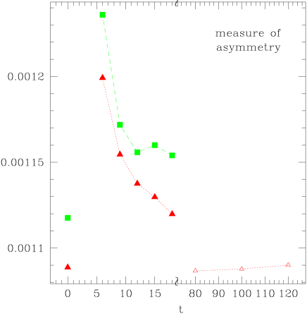
Figure 2: Evolution towards stationarity as measured by the symmetry (13) for different models (arbitrary units, horizontal axis is time in bar rotation periods). Models shown have $R_{\mathrm{OLR}}/R_{0}=0.8$ (squares) and $R_{\mathrm{OLR}}/R_{0}=0.92$ (triangles), and usual (filled) or long integration time (open). Bar growth is taking place in the first 5 periods for normal and in the first 10 periods for the long integration time. In addition, the value for the sampled starting distribution at $t=0$ is shown, indicating the noise level.

2.4 Fourier Components of Velocity Moments

In order to most easily follow the evolution of the disk, it is useful to do a Fourier transform on the azimuthal angle $\varphi$. We apply this to the mean velocities and dispersion tensor elements after we calculated these in the usual way (9), except that this time we do not use a weighting function, but take bins in $R$ and $\varphi$ to make sure every calculated trajectory contributes to the final result. We use a discrete Fourier transform of the following kind:

$$\begin{array}[]{lll}c_{m}&=&\displaystyle\frac{2}{N}\sum_{j=1}^{N}f(\varphi_{j})\cos m\varphi_{j},\\[8.61108pt] s_{m}&=&\displaystyle\frac{2}{N}\sum_{j=1}^{N}f(\varphi_{j})\sin m\varphi_{j},\end{array}$$ (11)

where $\varphi_{j}=j\pi/N$. This gives an approximate Fourier expansion

$$f(\varphi)\approx\frac{c_{0}}{2}+\frac{c_{n}}{2}\cos n\varphi+\sum_{m=1}^{n-1}(c_{m}\cos m\varphi+s_{m}\sin m\varphi),$$ (12)

where $n=N/2$ and $N$ is supposed to be even. This has been done for $N=32$ in 25 radial bins.

We also construct an estimate of the surface density $\Sigma$ by dividing the number of sampled orbits per bin by the segment area of the bin, and apply the Fourier transform to this quantity as well.

2.5 Error Estimation

We employ a bootstrap method: the calculations leading from the data set of every radial bin to its Fourier coefficients are redone for arbitrary subsamples of this data set. The rms scatter in the outcome of many such calculations gives a measure of the error.

2.6 Symmetries and the Question of Stationarity

In order to check, whether or how far our distributions have reached a stationary equilibrium state, we employ a symmetry consideration. As noted by Fux (2001), velocity distributions in an $m=2$ symmetric potential have a symmetry

$$f(R,\varphi,u,v)=f(R,\pi-\varphi,-u,v),$$ (13)

which is a consequence of the azimuthal $m=2$ symmetry and the time-reversal symmetry of stellar dynamics in conjunction with stationarity of the distribution function. We can turn this argument around and use the degree of symmetry as a measure for stationarity. A quantitative measure of the symmetry can be obtained in the obvious way by subtracting corresponding distribution function values over a grid in phase space and doing a quadratic sum over the grid points. Results of this kind of analysis are shown in Fig. 2. As can be seen, the simulations show only a small increase in asymmetry of 15% above the noise level (as given by the initial state as well as a very long-time simulation), and this is dropping rapidly after bar growth is finished.

3 Results

Kuijken & Tremaine (1991) gave an analytical expression for the behaviour of the mean velocities under the influence of a non-axisymmetric perturbation of multipole order $m$ in a linear approximation. For our case, this yields

$$\bar{u} = \frac{\alpha(R)\,v_{0}^{2}}{3R}\frac{3\Omega_{b}-\Omega}{(\Omega-\Omega_{\mathrm{ILR}})(\Omega-\Omega_{\mathrm{OLR}})}\sin 2\varphi,$$

$$\bar{v} = v_{0}-\frac{\alpha(R)\,v_{0}^{2}}{6R}\frac{4\Omega_{b}-\Omega}{(\Omega-\Omega_{\mathrm{ILR}})(\Omega-\Omega_{\mathrm{OLR}})}\cos 2\varphi,$$

where $\Omega_{\mathrm{ILR}}$ and $\Omega_{\mathrm{OLR}}$ refer to the circular frequencies at the radii of the inner and outer Lindblad resonance. For a flat rotation curve, $\Omega=v_{0}/R$. In our range of interest, Eqs. (3) are dominated by a pole at the OLR.

The results of our simulation, presented below, agree roughly with these expectations: the mean velocities show modulations $\bar{u}\propto\sin 2\varphi$, $\bar{v}\propto\cos 2\varphi$. The sign of the modulations varies with radius, sign changes should indicate resonances. For the dispersion tensor the situation is similar: the off-diagonal component shows a $\sin 2\varphi$ perturbation, the diagonal components a $\cos 2\varphi$.

3.1 Fourier Analysis

Since we have an azimuthal $m=2$ symmetry, all coefficients of odd index $m$ are expected to vanish, what they do within their errors. Furthermore, in the undeveloped state before bar growth, all coefficients except those with $m=0$ are, by construction, zero within their errors.

3.1.1 The $m=0$ Components:

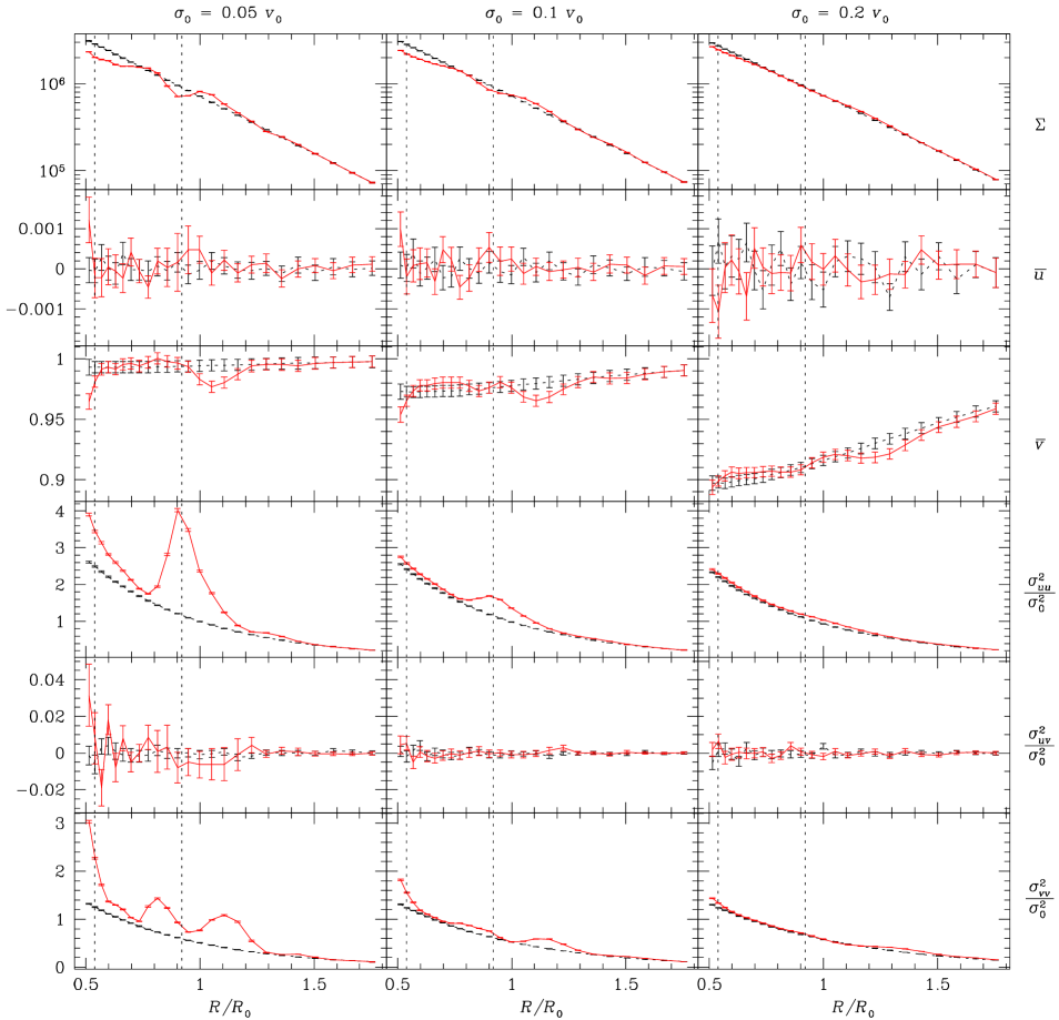
Figure 3: Axisymmetric ($m=0$) components of velocity distribution in the undeveloped state before bar growth (dashed) and in the final state (solid), plotted against radius. Results for models with initial $\sigma_{0}=0.05v_{0}$, $0.1v_{0}$ and $0.2v_{0}$ are shown in the left, middle and right panels, respectively. Velocities are given in units of $v_{0}$ and $\Sigma$ in arbitrary units. The model shown has an OLR-radius of $0.92R_{0}$, corresponding to a CR of $0.539R_{0}$ (dashed vertical lines).

The dashed lines in Fig. 3 represent the initial axisymmetric case, which shows an exponential decline of $\Sigma$ as well as in the diagonal components of velocity dispersion tensor. The mean azimuthal motion deviates from the circular speed $v_{0}$ by the asymmetric drift, which is stronger for large $\sigma_{0}$, as expected. The mean radial motion vanishes, as required for any stationary model.

The solid lines in Fig. 3 show the radial run of the $m=0$ components in the barred case. Apart from the components for $\bar{u}$ and $\sigma^{2}_{uv}$, which have to vanish for stationary models, some signs of perturbation are visible, the stronger the smaller $\sigma_{0}$.

First of all, we learn that dispersive effects are quite efficient in drawing resonance-induced features away from the actual position of the resonance. Whereas for small velocity dispersion the association of the features with the OLR at $R_{\mathrm{OLR}}=0.92R_{0}$ is clearly visible, they appear in the high dispersion case at a radial range of $1.1$ to $1.4R_{0}$, where naively one would not attribute them to the OLR.

In particular, we have a bump in the $\bar{v}$-curve outside of OLR, which becomes more explicit with decreasing dispersion while roughly keeping its absolute magnitude. In contrast to this, the asymmetric drift as the dominant deviation of $\bar{v}$ from the nominal rotation velocity $v_{0}$ diminishes with decreasing dispersion. There is a similar bump in $\sigma_{uu}^{2}$, whereas we have a two-fold feature in $\sigma_{vv}^{2}$.

Most of the perturbative features in the $m=0$ components are induced by the opposite orientation of the near-circular orbits on either side of the resonance.

3.1.2 The $m=2$ Components

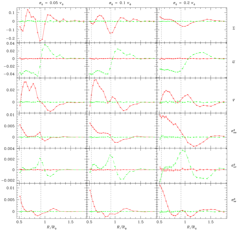
Figure 4: $m=2$ Fourier cosine (solid) and sine (dashed) components, plotted against radius. Panels as in Fig. 3. For surface density $\Sigma$, the value shown is relative to the undisturbed $m=0$ value. OLR and CR are at $0.92R_{0}$ and $0.539R_{0}$ respectively (dashed vertical lines).

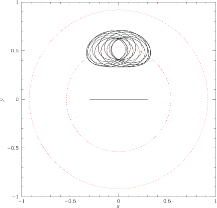
Figure 5: Orbit near co-rotation that circulates the L₄ point in a retrograde sense (anti-clockwise for a clockwise rotating bar). The bar is indicated by a line, while the dotted circles correspond to CR and OLR. In our model, a considerable fraction of stars is trapped in orbits of this family, resulting in the somewhat peculiar run of the velocity moments (Fig. 4).

Because of the symmetry of the problem, we expect the $m=2$ components to be the dominant ones. As for every $m>0$, we have one more degree of freedom here, since we have a cosine- and a sine-component (see Fig. 4), or equivalently, an amplitude and a phase.

The cosine-terms of $\bar{u}$ and $\sigma^{2}_{uv}$ as well as the sine terms of $\Sigma$, $\bar{v}$, $\sigma^{2}_{uu}$, and $\sigma^{2}_{vv}$ vanish (within their error), which is to be expected from Eq. (13) for a stationary model. The behaviour of the remaining non-vanishing terms agrees roughly with the expectation from simple linear theory, cf. Eq. (3). However, there are two significant deviations. First, as $\sigma_{0}$ increases (from left to right panels in Fig. 4), the resonant features are shifted away from $R_{\mathrm{OLR}}$ to larger radii and are also somewhat smoothed out. Second, there is an additional feature at $R\sim 0.6R_{0}$, in particular, for $\bar{v}$. When inspecting the orbits of stars dominating at this radius, we find that many belong to an orbit family associated with the stable Lagrange points L₄ and L₅, see Fig. 5. These orbits can reach radii far beyond co-rotation and, in a frame co-rotating with the bar, perform a retrograde motion around the Lagrange points. They thus result in a reduced $\bar{v}$ at azimuths perpendicular to the bar and hence lead to a positive $\cos 2\varphi$ component.

3.1.3 Higher-Order Components

The $m=4$ components are usually smaller by at least a factor 3 compared to the $m=2$ modes, but they are significantly different from zero. In contrast, the analytical model (3) had no excitation of higher modes at all, since mode coupling is not included in a linear approximation.

The excitation of the $m=4$ modes follows the overall pattern seen in the $m=2$ case: in accordance with the symmetry requirements, we have a $\sin(4\varphi)$ in $u$ and $\sigma_{uv}^{2}$, and a $\cos(2\varphi)$ in all the other components. Our signal-to-noise ratio is in the range of about 3 for the $m=4$ case, and less for higher components, so surely the significance of our model is petering out. Nevertheless, some $m=8$ modes do seem to be discernible still.

3.2 Variation of Parameters

Doubling the bar strength leads to a doubling of the magnitude of the effects. This is true for the differences between the undeveloped and final state as well as for Fourier coefficients.

Changing the bar size, i.e. the parameter $R_{b}$ in (5), produces some local variations in the magnitude of the effects, but it does not shift them in location. Of course, this is to be expected if the location is determined by resonance conditions.

Variation of the disk scale length does not seem to have any strong effects, which is to be expected, since it only slightly affects the sampling of the orbits but not the dynamics.

The shape of the velocity curve has a mild effect: we tried models with a slightly rising ($\beta=0.1$) or falling ($\beta=-0.1$) velocity profile, and found very similar results as for $\beta=0$. (Note that we kept the OLR radius fixed, so models with different velocity profiles have different rotation frequencies of the bar.) This is expected, too, since $\beta$ essentially controls the distances between various resonances (growing wider for larger $\beta$), while most of our results are dominated by a single resonance, the OLR.

3.3 The Axis Ratio of the Velocity Ellipsoid

Fig. 6 shows the ratio of the principal axes of the velocity dispersion ellipsoid, i.e. the eigenvalues $\sigma^{2}_{1,2}$ of the tensor $\boldsymbol{\sigma}^{2}$. For a flat rotation curve, this ratio is often expected to be 0.5. Indeed, in the undisturbed case (for which $\sigma_{1}=\sigma_{uu}$ and $\sigma_{2}=\sigma_{vv}$)

$$\lim_{\sigma\rightarrow 0}\frac{\sigma_{2}^{2}}{\sigma_{1}^{2}}=\frac{\kappa^{2}}{4\Omega^{2}}\equiv\frac{1}{2}\left(1+\frac{d\ln v_{c}}{d\ln R}\right),$$ (15)

where $\kappa$ is the epicycle frequency. This relation is often given without the limit and then referred to as Oort’s relation. It is, however, important to note that the error in Oort’s relation is considerable already for $\sigma_{0}=0.2v_{0}$ (Evans & Collett, 1993; Dehnen, 1999), which means that using it for the old stellar disk of the Milky Way is, at best, dangerous. This can be seen clearly from Fig. 6 showing that $\sigma_{2}^{2}/\sigma_{1}^{2}$ for the unperturbed case (dotted) significantly deviates from 0.5 for a warm stellar disk ($\sigma_{0}=0.2v_{0}$).

After formation of the bar perturbation, we have large variations in this quantity. For $\sigma_{0}=0.2v_{0}$ and at $R=R_{0}$, the values are generally somewhat higher than Oort’s value 0.5 but smaller than for an undisturbed disk. For directions that are roughly along the bar ($\varphi\sim 0$), this ratio rises sharply just outside the solar circle to values reaching as high as 0.8.

It is instructive to take a look at the same quantities for a smaller velocity dispersion of $\sigma_{0}=0.05v_{0}$ or $0.1v_{0}$ (left and middle panels of Fig. 6). First of all, the axis ratio in the undisturbed case (dashed line in the right panels) is much closer to Oort’s value of 0.5 here, as expected. Generally, the observed features have smaller width, i.e. they are less washed out by dispersion, but the effect of the bar, i.e. the difference between the solid and dashed lines, is still even quantitatively similar for the different velocity dispersions. Thus, the deviation of $\sigma_{2}^{2}/\sigma_{1}^{2}$ from Oort’s value may be decomposed into a velocity-dispersion dependent term, which consists of a general elevation of only mild radial dependence and a bar-induced term, which varies spatially and appears to be negative for the Solar position.

As a consequence, for mildly warm stellar disks ($\sigma\la 0.2v_{0}$), the ratio $\sigma_{2}^{2}/\sigma_{1}^{2}$ in the Solar neighbourhood may well drop below Oort’s value.

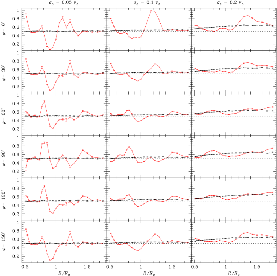
Figure 6: Axis ratio $\sigma^{2}_{2}/\sigma^{2}_{1}$ of the principal components of the velocity-dispersion tensor for the final (solid) and the initial unperturbed state (dashed) at various azimuths for the models with $R_{\mathrm{OLR}}=0.92R_{0}$ and $\sigma_{0}$ of $0.05v_{0}$ (left), $0.1v_{0}$ (middle), and $0.2v_{0}$ (right)

Figure 7: Vertex deviation $\ell_{v}$ at various azimuths for the same models as in Fig. 6. The highly uncertain outliers at $R\sim 1.2R_{0}$, $\varphi=0\degr$ for $\sigma_{0}=0.1v_{0}$ are caused by a near-circular velocity ellipsoid ($\sigma_{1}\sim\sigma_{2}$, see Fig. 6), which renders the vertex deviation ill-defined.

3.4 Vertex Deviation

The so-called vertex deviation

$$\ell_{v}=\frac{1}{2}\arctan\frac{2\sigma_{uv}^{2}}{\sigma_{uu}^{2}-\sigma_{vv}^{2}}$$ (16)

is the angle between the direction of the largest velocity dispersion and the line to the Galactic center, see also Fig. 1. For axisymmetric equilibrium models, $\ell_{v}=0$.

In Fig. 7, we plot $\ell_{v}$, computed from Fourier coefficients up to $m=2$ only in order to eliminate short-scale fluctuations. We find that the bar-induced vertex deviation decreases with increasing velocity dispersion from up to $\sim 30\degr$ for $\sigma_{0}=0.05v_{0}$ to $5\degr$ – $10\degr$ for $\sigma_{0}=0.2v_{0}$. In the direction of the bar and perpendicular to it, $\ell_{v}=0$, as expected from symmetry. For moderately warm stellar disks ($\sigma_{0}\ga 0.1v_{0}$) the vertex deviation at azimuth angles between $0^{\circ}$ and $90^{\circ}$ (including the Solar azimuth) is positive at and inside the solar circle and negative for some range outside. The actual radius where the sign change occurs is obviously coupled to the OLR, but again shifted to the outside. For a cold stellar disk, the bar-induced vertex deviation displays are more complicated pattern and may reach as high as $40\degr$.

Obviously, the vertex deviation is antisymmetric with respect to $\varphi\mapsto(\pi-\varphi)$, whereas the velocity dispersion axis ratio is symmetric. This is a simple consequence of symmetry (13), which in particular implies $(\sigma^{2}_{uu},\sigma^{2}_{uv},\sigma^{2}_{vv})\mapsto(\sigma^{2}_{uu},-\sigma^{2}_{uv},\sigma^{2}_{vv})$.

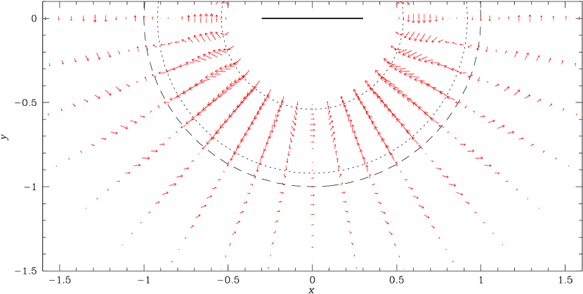
Figure 8: Bar-induced deviations of the mean velocity from the unperturbed state up to $m=2$ for $\sigma_{0}=0.2v_{0}$. The bar is aligned with the horizontal axis and is supposed to rotate clockwise. The solar circle is dashed, dotted circles are CR and OLR.

4 Discussion

We have studied the bar-induced variations of the mean velocities and velocity dispersions in the outer disk of a barred galaxy with special emphasis on the situation in the Milky Way. We generally find that these variations are largest near the outer Lindblad resonance (OLR), the apparent radius of which, however, may be shifted outwards by 10-20% due to the non-circularity of the orbits in a warm stellar disk.

Radial motions $\bar{u}$ of standards of rest can be seen to occur quite frequently (see Fig. 8), and can reach magnitudes of the order of about $0.02v_{0}$, corresponding to about 5 km s^-1 for the Milky Way. Because of the $\sin 2\varphi$ dependence, these would be maximal at $\varphi=45\degr$, which is quite near the proposed position of the Sun of $\varphi\approx 30\degr$. In its radial dependence however, $\bar{u}$ swings through zero shortly outside of the OLR, and it may well be that the Sun just meets that point. So we cannot give a definite prediction for the bar-induced radial motion of the LSR here, not even by sign only, except that it should be very small (at most a few km s^-1).

Variations of the mean azimuthal velocity are also present, but here we have to deal with several perturbation effects, the dominant one for realistic cases being traditional axisymmetric asymmetric drift. We can construct a picture of the bar-induced $\bar{{\boldsymbol{v}}}$-modifications only (see Fig. 8) by subtracting $\bar{{\boldsymbol{v}}}$ in the undeveloped case before bar growth, thus also canceling asymmetric drift. However, this is, of course, impossible for real galaxies, where only the combination of circular speed (LSR motion), asymmetric drift, and bar induced drift is measurable (in principle). In observational data, the effect of asymmetric drift can be corrected for, as done by Dehnen & Binney (1998), by calculating $\bar{v}$ for stellar populations with different velocity dispersions and extrapolating to vanishing dispersion. This approach, however, cannot be applied to the bar-induced perturbations in $\bar{v}$, since, as can be seen in Fig. 3, the relative magnitude of the bar-induced wiggle keeps constant at about 2%, independent of velocity dispersion. So, as long as only local measurements are available, there is no way to discern the bar-induced azimuthal velocity perturbations from variations in the background rotation curve, and so it will be rather hard to draw any observational constraints from the mean azimuthal velocities.

For an axisymmetric equilibrium, the no vertex deviation, i.e. $\ell_{v}=0$, is expected, while in the Solar neighbourhood $\ell_{v}$ is observed to drop from $\ell_{v}\approx 30\degr$ for blue to $\approx 10\degr$ for red main-sequence stars (Dehnen & Binney, 1998). The traditional interpretation of these vertex deviations is that young stars deviate from equilibrium, and thus even in an axisymmetric galaxy give rise to $\ell_{v}\neq 0$, which due to the decreasing number of young stars at later stellar types is a decreasing function of stellar colour.

Our calculations show that for an equilibrium in a barred Milky Way, with bar orientation, strength and pattern speed consistent with other data, a vertex deviation of the size and direction as observed emerges naturally. Moreover, we also found that for dynamically cooler sub-populations, i.e. bluer or younger stars, the bar-induced vertex deviation increases in amplitude, very similar to the observed values.

This gives strong support for the hypothesis that the vertex deviation observed in the Solar neighbourhood is predominantly caused by deviations from axisymmetry rather than from equilibrium. This explanation also naturally accounts for the fact that $\ell_{v}$ for young stars has the same direction as for old ones, which with the traditional explanation would be a chance coincidence.

The axis ratio of the (principal components of the) velocity dispersion tensor, $\sigma_{2}^{2}/\sigma_{1}^{2}$, is clearly affected by the central bar. In particular, values less than 0.5, Oort’s value for a flat rotation curve, are possible (Oort’s value is a lower limit for an axisymmetric galaxy, see Sect. 3.3 and Evans & Collett, 1993; Dehnen, 1999). This nicely fits to the values inferred from HIPPARCOS data (Dehnen & Binney, 1998), which give $\sigma_{2}^{2}/\sigma_{1}^{2}\sim 0.42$ for the old stellar disk.

In the Milky Way, as well as in many barred galaxies, the bar is not the only deviation from a smooth axisymmetric background. Most prominently, spiral arm structure and an elliptic (or oval) disk and/or halo add further non-axisymmetric perturbations. However, we will defer the discussion of the influence of spiral arms on the outer disk kinematics to a future paper.