Tidal Effects in Clusters of Galaxies

Abstract

High-redshift clusters of galaxies show an over-abundance of spirals by a factor of $2-3$, and the corresponding under-abundance of S0 galaxies, relative to the nearby clusters. This morphological evolution can be explained by tidal interactions with neighboring galaxies and with the hierarchically growing cluster halo. The efficiency of tidal interactions depends on the size and structure of the cluster, as well as on the epoch of its formation. I simulate the formation and evolution of Virgo-type clusters in three cosmologies: a critical density model $\Omega_{0}=1$, an open model $\Omega_{0}=0.4$, and a flat model $\Omega_{0}=0.4$ with a cosmological constant. The orbits of identified halos are traced with a high temporal resolution ($\sim 10^{7}$ yr). Halos with low relative velocities merge only shortly after entering the cluster; after virialization mergers are suppressed.

The dynamical evolution of galaxies is determined by the tidal field along their trajectories. The maxima of the tidal force do not always correspond to closest approach to the cluster center. They are produced to a large extent by the local density structures, such as the massive galaxies and the unvirialized remnants of infalling groups of galaxies. Collisions of galaxies are intensified by the substructure, with about 10 encounters within 10 kpc per galaxy in the Hubble time. These very close encounters add an important amount (10–50%) of the total heating rate. The integrated effect of tidal interactions is insufficient to transform a spiral galaxy into an elliptical, but can produce an S0 galaxy. Overall, tidal heating is stronger in the low $\Omega_{0}$ clusters.

1 Introduction

This work is motivated by the wealth of recent observational discoveries of the strong morphological, chemical, and dynamical evolution of galaxies in clusters. Transformations of luminous galaxies, the existence of separate massive dark objects, and the evolution of cluster substructure intensify the need for theoretical understanding. Several different phenomena have been proposed as the “likely” explanation (see §2). While all of them take place in one form or another, it has eluded our understanding which process is primarily responsible for the evolution.

I argue that tidal interactions with neighboring galaxies and with the dark cluster halo are the favored scenario. Tides operate even before the cluster dynamically relaxes and affect both stars and gas in the infalling galaxies. Tidal effects add enough random motion to transform thin galactic disks into the kinematically hot thick-disk configurations characteristic of S0 galaxies. Tidal disruption of low density galaxies may provide a large fraction of the diffuse intracluster light.

The relative importance of tides depends on the cosmological context. In an $\Omega_{0}=1$ universe, gravitating structures assemble late and the tidal effects are only now starting to play a role in shaping the galaxies, whereas in an open universe, $\Omega_{0}\sim 0.4$, galaxies have formed early and experienced a substantial metamorphosis. The currently fashionable model, a flat universe with $\Omega_{0}=0.4$ and a cosmological constant, provides the intermediate case. In order to incorporate these effects into the galactic dynamics self-consistently, I perform numerical simulations of the evolution of a medium-size cluster of galaxies in the three cosmologies.

The choice of a numerical scheme is very important here, as the required dynamical range of simulation is huge: from hundred parsecs to model the galactic dynamics to tens of Mpc to derive the cluster tidal field correctly. In order to achieve such a range with the existing codes, I introduce a new scheme of separating the cluster tidal field from the galactic model. First, I run a lower resolution cosmological simulation that captures the details of cluster formation and its time-varying potential. At some early redshift, $z_{g}=5$, I identify the probable galactic halos and follow their trajectories until the present. Along each trajectory, I calculate and store the components of the tidal shear tensor. Then, I resimulate individual galaxies with a very high resolution applying the cluster tidal field as an external perturbation. The results of the stellar dynamical galaxy simulations are presented in a companion paper (Gnedin 2003, hereafter Paper II). No single simulation of a cluster of galaxies (§2.5) has been able to achieve comparable resolution on the galactic scale.

I describe a careful procedure to extract the tidal field from the grid PM simulation. Because of the particle noise, it is necessary to apply a smoothing filter extending over a range of several grid cells. Also, large halos contribute significantly to the tidal field around their centers. Since we are interested only in the external tidal force on the galaxy, this self-contribution needs to be removed. Special care is taken to evaluate the contribution of the galactic particles and subtract it from the total tidal tensor.

Also, the resulting tidal field depends on the correct calculation of the galactic trajectories. I use two independent methods to follow the trajectories: in one, the galactic centers of mass are assumed to be test particles following the overall cluster potential; in the other, the center of mass is calculated using the densest subset of particles constituting an actual halo. The sampling of halos at each time step provides an excellent time resolution of the tidal field, of order $10^{7}$ yr. Finally, the distribution of halos and their relative velocities enable us to estimate the contribution of close encounters to the external tidal force.

In §2, I review the present observational status of galaxies in clusters at various redshifts and the theoretical mechanisms connecting pieces of the puzzle. In §3, I describe the numerical method used to simulate the self-consistent evolution of the three clusters starting with the primordial fluctuations. In §4, I identify the galactic halos and calculate their trajectories. In §5, I study the possible mergers and close encounters between galaxies, including the effects of halo clustering. Finally in §6, I calculate the tidal field along the galaxy trajectories and use it in §7 to estimate the amount of tidal heating of galaxies.

2 Scenarios of Galactic Evolution

The idea that the environment plays a role in the evolution of galaxies has been recognized long ago. Spitzer & Baade (1951) suggested that collisions between galaxies might be responsible for transforming spirals into the gas-free S0s. Toomre (1977) advocated a merger of two spirals to produce an elliptical. Richstone (1976) argued for the truncation of dark matter halos of galaxies by the tidal field of the cluster. Gunn & Gott (1972) proposed the stripping of gas by the ram pressure of the intracluster medium. Finally, Merritt (1983) and most recently Moore at al. (1998,1999) considered tidal interactions between the galaxies and the dense cluster core and between the galaxies themselves. I review the observational picture and then discuss briefly the pros and cons of each of these scenarios.

2.1 “Spirals vs Ellipticals” or “Spirals vs S0s”?

The Hubble Space Telescope has been instrumental in shaping our current understanding of distant clusters of galaxies. The unique resolving power of the HST brings us exquisite details of the distorted profiles of the otherwise normal disk galaxies. Strongly depleted in nearby clusters, spirals make up to 50% of the galaxies in clusters at redshift $z\sim 0.5$ (Oemler et al., 1997; Ellis et al., 1997; Smail et al., 1997). These results are similar to the Butcher–Oemler (1978) effect, an abundance of blue irregular galaxies at an intermediate redshift. Spectroscopic evidence (Dressler et al., 1997) suggests bursts of recent, or even current, star formation. This picture is drastically different from the rich present-day clusters, populated mostly by featureless elliptical or S0 galaxies which follow the local morphology-density relation (Dressler, 1980). It is well established now that a strong chemical and morphological evolution has taken place in clusters of galaxies.

What are the options? Did the $z=0.5$ spirals become the $z=0$ ellipticals? On the contrary, the HST data show that the fraction of elliptical galaxies increases with redshift, although not as strongly as that of spirals. Both of these effects occur at the expense of S0s. Their population is depleted by a factor of two or three at $z\sim 0.5$ (Dressler et al., 1997). Observations suggest that star formation has ceased in the ellipticals by $z\sim 0.6$, but continued in the S0s at least until $z\sim 0.3$ (van Dokkum et al., 1998). The ellipticals must have exhausted their supply of fresh gas at an earlier time, as indicated also by their very high central densities (Kormendy, 1989).

Even at low redshift the situation is far from being smooth (Conselice & Gallagher, 1999). New ground-based imaging of the Coma and five other nearby clusters reveals a variety of distorted, tailed, “line”, and dwarf galaxies. These are indicators of the ongoing dynamical evolution. Many galaxies are disturbed and some show blue colors. Also, individual groups of dwarf galaxies have been found in Coma. These results were not expected for the smooth and regular clusters.

A new observational puzzle has been presented by the discovery of massive dark objects in the cluster CL 0024+1654, through the technique of image reconstruction of gravitational lensing (Tyson, Kochanski & Dell’Antonio, 1998; Kochanski, Dell’Antonio & Tyson, 1998). The dark objects are not associated with any of the luminous galaxies in the cluster and may contain as much mass as $10^{10}\,M_{\sun}$. One of the possible explanations is that these objects are just “failed” galaxies, in which gaseous dissipation was insufficient to form stars. Alternatively, they can be stripped dark matter halos of other galaxies. Analytical arguments and previous studies (§2.3) suggest that extended galactic halos may be effectively swept away by the tidal field of the cluster.

2.2 Mergers of Galaxies

Collisions of galaxies are assisted by the dense environment of the cluster. However, in a virialized cluster, galaxies move with the relative velocities of the order 1000 km s^-1 and even on a head-on trajectory will pass through each other without doing much harm to the stellar disks. The gas can be shocked and stripped away in such a collision (Spitzer & Baade, 1951), which would leave two gas-free galaxies. But a simple estimate argues that close encounters are very infrequent (however see §5 and Appendix A).

Consider a virialized cluster of galaxies with a one-dimensional velocity dispersion $\sigma_{cl}=1000$ km s^-1 and a virial radius $R_{cl}=1$ Mpc. Assuming that the cluster contains $N_{g}=1000$ galaxies uniformly distributed inside this radius, the number of close encounters a given galaxy of size $R_{g}=10$ kpc will experience in a Hubble time ($t_{H}=10^{10}$ yr) is

$$N_{\rm enc,1}\approx{N_{g}\over\frac{4\pi}{3}R_{cl}^{3}}\,\pi R_{g}^{2}\,\sqrt{2}\sigma_{cl}\,t_{H}\approx 1.$$ (1)

Here I have neglected gravitational focusing and assumed the relative velocity to be $\sqrt{2}\,\sigma_{cl}$. Thus a galaxy is expected to encounter one other galaxy over the course of its evolution. However, the probability of a merger of two galaxies is much smaller:

$$P_{\rm mer}\sim N_{\rm enc,1}\,\left({\sigma_{g}\over\sigma_{cl}}\right)^{4}\approx 10^{-3}$$ (2)

for the galactic velocity dispersion $\sigma_{g}=200\ {\rm km\ s}^{-1}$. Here, three powers of $\sigma_{g}/\sigma_{cl}$ come from the phase space density and another power of $\sigma_{g}/\sigma_{cl}$ comes from the limitation of the velocity that leads to a merger (Binney & Tremaine, 1987).

Also, ellipticals usually have much higher central densities than spiral galaxies. So if two spirals merge, it seems hard to close the gap in density without strong dissipation (Carlberg, 1986). As Jim Gunn once said (Gunn, 1987), “I do not think you can make rocks by merging clouds.” Thus the merger scenario appears unlikely to dominate the dynamics of galaxies, although mergers could be important for the formation of the central giant cD galaxy (Ostriker & Hausman, 1977; Merritt, 1985; Lauer, 1988) and the ultraluminous infrared galaxies and AGNs (e.g., Canalizo & Stockton 2001).

2.3 Truncation of Dark Matter Halos

Richstone (1976), White (1976), and Merritt (1983), among others, have investigated the truncation of dark galactic halos by the tidal field of the cluster. In the simplest case, where both the cluster and the galaxy halos have singular isothermal distributions, the tidal radius is approximately

$$R_{t}\approx{\sigma_{g}\over\sigma_{cl}}\,R_{p},$$ (3)

where $R_{p}$ is the distance of closest approach to the center of the cluster.

Real clusters are not perfectly smooth. Any substructure left after the hierarchical formation of the cluster will amplify the truncation effect. It is expected to control the amount of dark matter, and therefore, the mass of the galaxies. On the other hand, tidal truncation should not significantly affect the dynamics of the galactic disks which are much more compact. Morphological evolution of luminous galaxies must be due to something else.

2.4 Ram-Pressure Stripping of Gas

Gunn & Gott (1972) argued that the ram pressure of the intracluster medium (ICM) might sweep away gas from the galactic disks. X-ray observations show the presence of a significant amount of hot gas at the virial temperature, contributing as much as 10% of the total cluster mass. While the stars move freely through this media, the gas is subject to the ram pressure $P_{\rm ram}\approx\rho_{\rm icm}v^{2}$, where $\rho_{\rm icm}$ is the density of the ICM and $v\sim\sigma_{cl}$ is the velocity of the galaxy. In order to strip the gas, the ram pressure should exceed the restoring gravitational force per unit area of the disk:

$$\rho_{\rm icm}v^{2}>2\pi G\,\Sigma_{s}\,\Sigma_{g},$$ (4)

where $\Sigma_{s}$ is the surface density of the stars, and $\Sigma_{g}$ is the surface density of the gas. For example, if the gas with an average density 1 cm^-3 is distributed over a scale height of 100 pc and the stellar density is typical of the solar neighborhood, $\Sigma_{s}\approx 75\ M_{\sun}$ pc^-2, the ICM needs to be as dense as $n_{\rm icm}>4\times 10^{-4}$ cm^-3. Such densities are observed in the cores of rich clusters, and numerical experiments (Kundić et al., 1993; Abadi, Moore & Bower, 1999; Quilis, Moore & Bower, 2000) show that a typical spiral there may lose most of its atomic gas.

Spiral galaxies in clusters have long been known to be deficient of atomic hydrogen (Krumm & Salpeter, 1976; Haynes, Giovanelli & Chincarini, 1984). These “anemic” galaxies (van den Bergh, 1991) have normal molecular hydrogen abundances but lack the atomic component in the outer parts of their disks. Since the H₂ gas resides in dense molecular clouds, it is more able to withstand the external pressure; on the other hand, the H i gas is usually distributed much more smoothly at lower densities and is susceptible to the ram pressure stripping. But Valluri & Jog (1991) noticed an interesting feature in three rich Abell clusters and the Virgo cluster: the H i deficiency is stronger for larger galaxies. Since bigger spirals (excluding the LSBs) usually have a higher surface density, they should be able to protect their gaseous component better. The observed trend is the opposite. Having considered various possible mechanisms of gas removal, Valluri and Jog conclude that the H i deficiency can only be explained by tidal interactions.

2.5 Tidal Interactions

Tides are a critical factor of the cluster environment. Tidal effects depend on relative sizes of the system and the perturber. Consider stellar systems from smallest to largest scales: stars are $10^{8}$ times smaller than star clusters and experience almost no tidal effects (except in close binaries). Star clusters are $10^{4}$ times smaller than galaxies and experience significant tidal effects, which however operate on a long time scale (Gnedin & Ostriker, 1997). In contrast, galaxies are just 30 to 100 times smaller than clusters of galaxies. There tidal effects ought to be important!

Semi-analytic models of galactic encounters (Merritt, 1983) predict the segregation of galaxies by mass and the formation of a central cD galaxy. The giant cD grows by swallowing other massive galaxies in a process that widens the gap between the first and the second ranking galaxies (Ostriker & Hausman, 1977). Mass segregation in clusters is also supported by numerical simulations (Frenk et al., 1996). Recently, Dubinski (1998) confirmed that the central galaxy, rising by mergers of its neighbors, follows a de Vaucouleurs profile and would be classified as a giant elliptical.

Restricted numerical simulations of Byrd & Valtonen (1990) and Valluri (1993) show that tidal compression by the cluster halo produces spiral arms and tidal tails in some of the representative models of disk galaxies.

More recently, Moore at al. (1996b,1998) simulated the dynamics of galaxies in a fixed, isothermal cluster. They found that fast close encounters with massive galaxies tend to destroy many dwarfs, and even large galaxies lose their thin disks. So the spiral galaxies are essentially transformed into the ellipticals or dwarf spheroidals. However, the potential of a real cluster grows in time, which leads to two competing effects: (1) galaxies enter the cluster at a later epoch and have less time to interact (depending on cosmological model), and (2) the time-varying cluster potential gives rise to large-scale perturbations in the tidal field and causes tidal shocks comparable to those from massive galaxies. New simulations by Moore at al. (1999) include the hierarchical cluster formation and show weaker evolution of galaxies. Whether the galaxy–galaxy or the cluster–galaxy interactions dominate has not yet been understood.

Similar tidal effects operate on smaller scale in the Local Group and may lead to the morphological evolution of the dwarf satellite galaxies (Mayer et al., 2001).

3 Numerical Method

I use a Particle-Mesh code (Cen, 1992) to simulate the formation and evolution of three clusters of galaxies in the critical ($\Omega_{0}=1$), open ($\Omega_{0}=0.4$), and flat ($\Omega_{0}+\Omega_{\Lambda}=1$) cosmological models described in Table 1. The code solves Poisson’s equation using FFT on a rectangular grid and evaluates the density field using the Cloud-in-Cell (CIC) method. The code runs fast in parallel, allowing a large simulation with $256^{3}$ particles distributed on a $512^{3}$ grid. Some of the PM results have been tested with the Adaptive Mesh Refinement code (Bryan et al., 1995). Specifically, I checked galaxy trajectories and the calculation of the tidal force.

The comoving size of the simulation box is $32\,h^{-1}$ Mpc and the grid cell size is $\Delta=62.5\,h^{-1}$ kpc. This is a compromise between the desire to reach a reasonably high resolution in the cluster center and the need to have enough computational volume to include late infall. The latter is important because a very strong initial density perturbation may lead to more mass being bound to the cluster than is available in the whole box, $9.1\times 10^{15}\,\Omega_{0}h^{-1}\,M_{\sun}$, causing the cluster to “under-form”.

Tests with different amplitudes of the power spectrum, $\sigma_{8}$, show that the dark matter velocity dispersion artificially saturates for $\sigma_{8}\gg 1$ in the low $\Omega_{0}$ models. Therefore, I adopt $\sigma_{8}=1$ for these models, in rough agreement with the relation derived from the comparison of large scale N-body simulations with the all-sky survey of X-ray clusters, $\sigma_{8}\approx 0.5\,\Omega_{0}^{-0.5}$ (Eke, Cole & Frenk, 1996; Pen, 1998). Then the virial mass of the simulated clusters is about $4\times 10^{14}\,M_{\sun}$, or 7% of the total mass within the computational box. The actual amount of mass bound to the clusters may be a factor of 2–3 higher, up to 20% of the total mass. In the critical density model, the normalization $\sigma_{8}=0.5$ is chosen such that the cluster velocity dispersion is the same as in the other two models.

The simulations start at redshift $z_{i}=20$. The time step is determined by the requirement that no particle crosses more than a half of the grid cell, $0.5\Delta$. Also, it limits the expansion parameter $a\equiv(1+z)^{-1}$ to grow by no more than $0.05(1+z_{i})^{-1}$. I have checked that increasing the time step by a factor of two does not change noticeably the structure of the resulting cluster.

The look-back time as a function of redshift (Peebles 1993, p. 314) can be calculated analytically in each of the three models. For $\Omega_{0}=1$, the standard result is $H_{0}\,t(z)={2\over 3}\,(1+z)^{-3/2}$. For $\Omega_{\Lambda}=0$,

$$H_{0}\,t(z)={(1+\Omega_{0}z)^{1/2}\over(1-\Omega_{0})(1+z)}+{\Omega_{0}\over 2(1-\Omega_{0})^{3/2}}\,\ln{f^{1/2}-1\over f^{1/2}+1},\;\;\;\;f\equiv{1+\Omega_{0}z\over 1-\Omega_{0}}.$$ (5)

For $\Omega_{0}+\Omega_{\Lambda}=1$,

$$H_{0}\,t(z)={2\over 3(1-\Omega_{0})^{1/2}}\,\ln{1+(1+f)^{1/2}\over f^{1/2}},\;\;\;\;f\equiv{\Omega_{0}\over 1-\Omega_{0}}\,(1+z)^{3}.$$ (6)

The Hubble constant is assumed to be $H_{0}=65$ km s^-1 Mpc^-1 ($h=0.65$), according to the time delay measurements in a gravitational lens system 0957+561 (Kundić et al., 1997) and other independent methods (Freedman et al., 1994).

On 16 processors of SGI Origin 2000, the full simulation with a $512^{3}$ grid runs for about 36 hours. A large fraction of the time is spent on the calculation of the tidal field due to and around the identified halos. All simulations presented in this paper were done using the 64-processor SGI Origin 2000 supercomputer at the Princeton University Observatory.

3.1 Constrained Initial Conditions

The cluster simulations use the constrained Gaussian random initial conditions, generated using the method of Hoffman & Ribak (1991). The actual realization is taken from the cluster comparison project of Frenk et al. (1999). In that work the initial density perturbations were chosen to produce a $3\sigma$ peak with a Gaussian filter of radius $5\,h^{-1}$ Mpc. Retaining the same random phases from the original realization, I have renormalized the perturbations according to the power spectrum of the chosen cosmological models.

For each of the three models, I evaluate the power spectrum $P(k)_{\rm new}$, including the effects of baryons, using the fitting expressions of Bardeen et al. (1986) and Hu & Sugiyama (1996). On the cluster and sub-cluster scales, the power spectra follow approximately a power law $P(k)\propto k^{-2.5}$. Then I transform the initial displacements $d$ into the Fourier space and renormalize their amplitudes according to the new power spectrum:

$$d_{k}^{\rm new}=d_{k}^{\rm old}\,\left({P(k)_{\rm new}\over P(k)_{\rm old}}\right)^{1/2},$$ (7)

where the old power spectrum, $P(k)_{\rm old}$, is from Frenk et al. (1999). Both power spectra are normalized to the corresponding value of $\sigma_{8}^{2}(z_{i})$ at the initial redshift $z_{i}$. Finally, I transform the perturbation field back to real space and obtain the initial displacements for the dark matter particles.

3.2 Structure of the Clusters

The parameters of the resulting clusters are given in Table 2. The virialized region is taken to be a sphere originating at the cluster center, with a mean overdensity $\delta=200$. The average mass of the clusters is $4\times 10^{14}\,M_{\sun}$, and the one-dimensional velocity dispersion is 660 km s^-1.

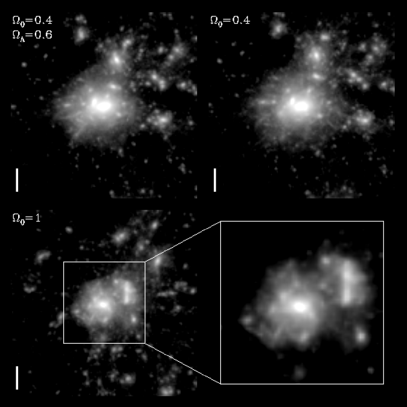
Figure 1: The surface density map of the three simulated clusters at $z=0$. The projection is over the $X$ direction. Saturated white regions are denser than 200 times the mean density; regions below the mean density are black. The size of the windows is $8\,h^{-1}$ Mpc. Thick bars in the lower left corner of each panel indicate $1\,h^{-1}$ Mpc. The lower right panel shows the enlarged view of the inner region of the $\Omega_{0}=1$ cluster.

Figure 1 shows the projected surface density of the three clusters at the present epoch. The $\Omega_{0}=1$ cluster has not yet relaxed and still continues to accrete matter. Note a large infalling group of galaxies to the upper right from the center on the enlarged panel. In contrast, the two low $\Omega_{0}$ clusters appear more spherical and regular, and also very similar to each other; the cosmological constant does not seem to affect the cluster properties.

Figure 2 shows that the density profiles of the three clusters are very similar, with a slight excursion of the $\Omega_{0}=1$ cluster at $r\approx 2\,h^{-1}$ Mpc due to the infalling group. This group is clearly visible on the velocity dispersion plot, Figure 3.

The decrease of the velocity dispersion at small distances from the center is partly real and partly numerical. The high resolution dark matter simulations in Frenk et al. (1999) show a similar decrease; therefore our models should exhibit the trend. Also, such a decrease exists in the popular NFW model (Navarro, Frenk & White, 1997). On the other hand, present simulations lack resolution in the cluster core and cannot be trusted at small radii. To illustrate the resolution effects, I have repeated the simulations of Cluster III on smaller grids, $256^{3}$ and $128^{3}$ cells (Table 3), with the correspondingly fewer particles, $N_{\rm grid}=2^{3}\,N_{\rm p}$. Figure 4 shows that the density profile is reproduced well to the resolution limit of each simulation, but the velocity dispersion starts to decline much earlier in the lower resolution runs. Nevertheless, the difference between the $512^{3}$ and the $256^{3}$ runs is small and confirms the accuracy of the larger simulation.

The simulated clusters are similar to the Virgo cluster in size and velocity dispersion. ROSAT results (Böhringer, 1994) indicate that Virgo’s X-ray mass is $(1.5-5.5)\times 10^{14}\,M_{\sun}$, while the optical velocity dispersion of galaxies is between 581 and 721 km s^-1 (Huchra, 1985). These values are quite common for the nearby clusters, as shown by the optical and X-ray survey of Girardi et al. (1998). Often cited in theoretical work, the Coma cluster is much larger, with the one-dimensional velocity dispersion about 1000 km s^-1 (Merritt & Gebhardt, 1994) and the virial mass of order $2\times 10^{15}\,M_{\sun}$ (Böhringer, 1994). Our models, therefore, represent modest but more common clusters of galaxies. Their velocity dispersion is characteristic of the Abell richness class 1 (see Postman, Huchra & Geller 1992).

4 Galaxies in the Simulation

The definition of a galaxy in the cluster simulation is not trivial. While at high redshift dark matter halos are significantly denser than the surrounding media, at low redshift the density contrast effectively disappears. This effect is known as overmerging of halos (e.g., Moore, Katz & Lake 1996a; Klypin et al. 1999) due to the insufficient mass resolution. Therefore, it is difficult and, to some extent, uncertain to try to identify the galaxy halos from the particle distribution at all times. Instead, I have implemented the following simple procedure, which can be extended to a higher degree of sophistication.

I identify the dark matter halos at a time early enough that the density contrast is large, but late enough that galaxies are known to exist. A fiducial epoch at which the central parts of large galaxies are assumed to have formed is taken to be $z_{g}=5$.

In order to obtain a statistically significant sample, I choose 100 most massive halos identified by the group finding algorithm. Then, I add 100 massless particles to the PM simulation with the coordinates and velocities of the halo centers of mass. These new “galactic” particles do not affect either the density or the potential calculation but rather act as test particles. I follow the motion of these particles and output the tidal field along their trajectories at each time step.

By not using real particles to calculate galaxy trajectories, we effectively avoid the overmerging problem: the test particles will not merge even if they come very close to each other. The drawback is that due to a finite time step the test particles may gradually depart from the bulk of the galactic particles. To guard against this effect, I have also implemented another scheme.

The second scheme involves real particles constituting the halo. I calculate the halo density at each particle’s position using the same CIC kernel that is used in the main PM calculation. Then I take the densest subset of particles, 1/8 of the total, to calculate the center of mass directly. These dense particles presumably lie deep in the potential well of the halo and serve as robust indicators of the center. In case of the two galaxies merging, their centers defined this way would clearly indicate it. However, I do not attempt to resolve the internal structure of galaxies in these simulations and only trace their centers of mass.

4.1 Group Finding Algorithm

Dark matter halos are identified using the coordinate-free algorithm HOP proposed by Eisenstein & Hut (1998). It is similar in spirit to DENMAX (Gelb & Bertschinger, 1994) but uses densities at the particle positions instead of the regular grid. I have extended HOP by including a procedure for the removal of particles which are not gravitationally bound to the group. This procedure, similar to the SKID algorithm (Weinberg, Hernquist & Katz, 1997), is outlined below.

The gravitational energy of the particles in a group is calculated by direct summation of the Plummer potentials with a smoothing length corresponding to one grid cell of the cluster simulation. The kinetic energy includes the Hubble expansion term. The total energy per unit mass is

$$E_{i}={1\over 2}\left[\mbox{\bf v}_{i}-\mbox{\bf v}_{\rm com}+H_{g}(\mbox{\bf r}_{i}-\mbox{\bf r}_{\rm com})\right]^{2}-\sum_{j}{Gm_{p}\over((\mbox{\bf r}_{i}-\mbox{\bf r}_{j})^{2}+\epsilon^{2})^{1/2}},$$ (8)

where $m_{p}$, $\mbox{\bf r}_{i}$, $\mbox{\bf v}_{i}$ are the particle mass, physical coordinate, and velocity, respectively, and $H_{g}$ is the Hubble constant at redshift $z_{g}=5$. The index “com” refers to the center of mass of the group. The particles are unbound as follows. I find particle $m$ with the maximum energy and discard it, if $E_{m}>0$. I recalculate the center of mass using the remaining particles and update the potential energy. Then, I find a new highest energy particle and repeat the procedure. In the end, all remaining particles are bound or else the group is dispersed.

A straightforward implementation of the unbinding procedure works well, although somewhat slowly for groups containing more than $10^{4}$ particles. In the longest case, the unbinding algorithm took about 40 minutes on a single SGI R10000 processor.

The second part of the HOP algorithm, REGROUP, uses three different overdensity parameters to define the outer boundary of the group ($\delta_{outer}$), the saddle point for merging two groups together ($\delta_{saddle}$), and the minimum density of a viable group ($\delta_{peak}$). After some experimenting, I have chosen the following parameters to produce the reasonable-size halos: [$\delta_{outer},\delta_{saddle},\delta_{peak}$] = [15,45,50] for the $\Omega_{0}=1$ model, and [20,55,60] for the low $\Omega_{0}$ models. The different sets of parameters are necessary because of the different masses of particles ($m_{p}=5.4\times 10^{8}\,\Omega_{0}h^{-1}\ M_{\sun}$).

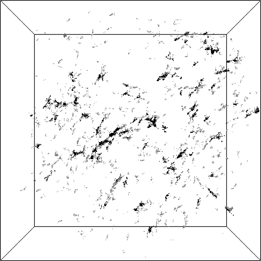
Figure 5: Three-dimensional distribution of particles in the identified halos at $z_{g}=5$ in the $\Omega_{0}=1$ cluster. The 100 most massive halos, whose trajectories are followed in the simulation, are black; others are gray. Boundary size is 16 $h^{-1}$ Mpc comoving.

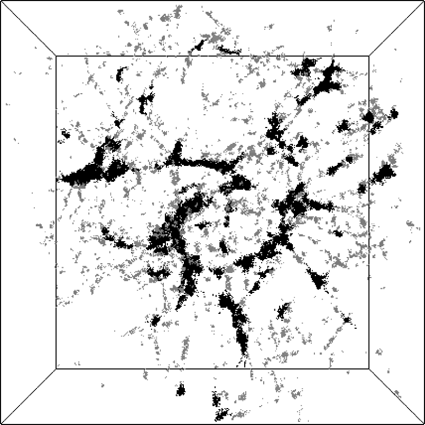
Figure 6: Particles in the identified halos in the $\Omega_{0}=0.4$ cluster.

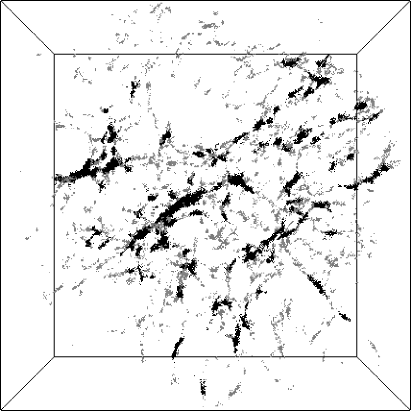
Figure 7: Particles in the identified halos in the $\Omega_{0}=0.4$, $\Omega_{\Lambda}=0.6$ cluster.

Figures 5–7 illustrate the location of particles in the identified halos. Notice the filamentary structure of bound particles indicating the directions along which the halos continue to assemble. Most galaxies in the central part of the simulation volume (shown on the Figures) fall eventually into the forming cluster. Because of the difference in particle masses, the $\Omega_{0}=1$ halos contain significantly fewer particles than the $\Omega_{0}=0.4$ halos.

4.2 Halo Mass Function

The mass function of the identified halos can be compared with the prediction of the Press-Schechter theory (Press & Schechter, 1974). I have calculated the expected number density of galaxies at $z_{g}$ using equations (A4-A9) of Mo, Mao & White (1998).

Figure 8 shows the halo mass functions in the three clusters. Note the relative depletion of low mass halos in the simulations. This is partly due to the truncation of the input power spectrum at the Nyquist frequency, which effectively prevents the formation of small-scale objects. For comparison, the lower right panel shows the mass function obtained in the lower resolution, $256^{3}$ simulation of Cluster III. As expected, the smaller halos are depleted more strongly than the larger ones.

4.3 Galaxy Trajectories

Figures 9–11 show the trajectories of two selected halos in each cluster. These galaxies are used for the high resolution simulations in Paper II, representing a large spiral and a dwarf spheroidal, respectively. Their trajectories are quite irregular. In the $\Omega_{0}=1$ case, the galaxies are just entering the cluster at the present epoch, although not on a free-fall path. The orbits are similar to those shown in Frenk et al. (1996). On the other hand, in the low $\Omega_{0}$ cases the galaxies have enough time to move around the cluster center several times, more so in the open model. These differences will have major effects on the dynamical evolution of the galaxies.

In general, there is a good agreement between the trajectories calculated using two different methods, especially for the less massive galaxies. For the very massive halos, the “test particle” motion occasionally tends to oscillate around the trajectory determined by the densest particle subset. I have therefore decided to use the latter as the more reliable trajectories.

5 Mergers and Close Encounters

The hierarchical formation of clusters and the survival of substructure lead to more frequent collisions of galaxies and lower relative velocities at early epochs. Preferentially radial infall implies that the final distribution of galaxies is very dense. Most of the galaxies lie close to the cluster center, while the rest form a scarcely populated halo.

The number density of massive galaxies ($M_{\rm min}\approx 10^{11}\,M_{\sun}$) can be fitted by a power law with a central core:

$$n_{g}(r)={n_{0}\over(r+r_{0})^{\gamma}},$$ (9)

normalized to the total number of galaxies $N_{g}$ within the virial radius of the cluster, $R_{\rm vir}$. Not all initially identified halos end up in the clusters, so with $N_{g}<100$ trying to estimate the core radius $r_{0}$ and the slope $\gamma$ by fitting a histogram of galaxy positions yields highly uncertain results. Instead, I use a maximum likelihood (ML) method analogous to that in Gnedin (1997). The parameters $r_{0}$ and $\gamma$ are to be determined by searching for the maximum of the ML function, ${\cal L}=e^{-N_{g}}\prod_{i=1}^{N_{g}}4\pi r_{i}^{2}n(r_{i})$. Requiring the two partial derivatives of $\log{\cal L}(r_{0},\gamma)$ to vanish gives a system of two integral equations, which have been solved numerically using the software package Maple. The resulting parameters are given in Table 4.

The slopes of the density profile are steep, $\gamma=2.4-4.2$. The massive galaxies are more concentrated in the inner parts of the clusters than the dark matter which follows an approximately isothermal profile, $\rho_{dm}\propto r^{-2}$. Also, the core radii in all three clusters are very small, below the force resolution scale. At such small distances from the center the distribution of galaxies can be affected by the giant cD galaxy which may swallow its neighbors. To check this, I have repeated the ML analysis excluding all galaxies within one resolution element, $\Delta$, from the center. This forces the core radii to be at least one $\Delta$. The resulting values (Table 4) are very close to this limit, suggesting that the true core radii can indeed be quite small. Thus the effect of the central giant on the overall galaxy distribution seems to be small.

5.1 Number of Close Encounters

The detailed trajectories of galaxies can be used to calculate the number of close encounters during the epoch of cluster formation. In order to detect all encounters, the trajectories are linearly interpolated between the successive time steps. The comoving separations are converted into physical kiloparsecs using the appropriate value of the Hubble constant at each time step. If a galaxy is found to have merged (see Appendix A), its subsequent trajectory is ignored.

Table 5 shows the number of encounters, $N_{\rm enc}$, as a function of the impact parameter, $R_{\rm enc}$. It is defined as a minimum distance between the centers of mass of the galaxies. The last column gives the “total” number of encounters for $R_{\rm enc}=40$ kpc (it is assumed that no mergers are possible for the separations larger than 40 kpc). Table 5 also shows the average number of close encounters per galaxy, $N_{\rm enc,1}$. Since each encounter involves two galaxies, this number is $N_{\rm enc,1}\equiv 2\,N_{\rm enc}/N_{g}$.

Figure 12 shows the number of collisions per galaxy within $R_{\rm enc}=20$ kpc. Note that in the low $\Omega_{0}$ clusters, most collisions take place near the end of the simulation, when the galaxies have assembled inside the cluster. In Cluster I, the galaxies are closer to each other initially and have close encounters uniformly distributed in time. Several distinct peaks, notably in Clusters I and III, can be due to the new groups of galaxies entering the clusters.

The number of close encounters does not scale very well with $R_{\rm enc}^{2}$, as predicted by equation (1). Since most encounters take place in the already formed cluster, any mergers prior to that remove prospective galaxies and reduce the number of subsequent collisions. To test that equation (1) would have been valid in the absence of mergers, I count the number of encounters disallowing mergers. The new numbers, $\tilde{N}_{\rm enc}$, scale as $R_{\rm enc}^{2}$ in agreement with the prediction (see Table 5).

However, the total number of encounters is much higher than expected. The effect is mainly due to the concentration of galaxies at the center of the cluster, implying a smaller effective volume. Equation (1) can be rewritten in a general form:

$$N_{\rm enc}=\int\pi R_{g}^{2}\,V_{\rm enc}\,t_{H}\,n_{g}^{2}(r)\,dV,$$ (10)

where the integration extends over the virial volume of the cluster, $V$. The mean value of the number density squared, $\langle n_{g}^{2}\rangle$, is substantially higher than the square of the mean density, $\langle n_{g}\rangle^{2}$, because of the galaxy clustering. Their ratio is the clumping factor

$${\cal C}\equiv{\langle n_{g}^{2}\rangle\over\langle n_{g}\rangle^{2}}={V\,\int n_{g}^{2}(r)\,dV\over\left(\int n_{g}(r)\,dV\right)^{2}}.$$ (11)

Using the azimuthally-averaged density profile (9) and the auxiliary functions

$$f_{n}(r_{0},\gamma)\equiv\int_{0}^{1}{x^{2}\,dx\over(x+r_{0}/R_{\rm vir})^{n\gamma}},$$ (12)

I find ${\cal C}={f_{0}f_{2}/f_{1}^{2}}$ (see Table 4). Now, the number of close encounters is

$$N_{\rm enc}=320\,\left({{\cal C}\over 1000}\right)\,\left({N_{g}\over 65}\right)^{2}\,\left({R_{cl}\over 2\ {\rm Mpc}}\right)^{-3}\,\left({R_{\rm enc}\over 10\ {\rm kpc}}\right)^{2}\,\left({V_{\rm enc}\over 800\ {\rm km\ s}^{-1}}\right).$$ (13)

This is much higher than the naive estimate (1) and agrees well with the results for Cluster III.

Because of the higher degree of clustering in the low $\Omega_{0}$ models, more than half of all encounters occur within the inner 0.4 Mpc from the center. In contrast, in the $\Omega_{0}=1$ model collisions take place throughout the cluster, leading to a smaller value of the clumping factor.

5.2 Relative Velocities

Figure 13 shows the relative velocities of galaxies at the time of collision. The distributions are skewed, peaking at low values and extending large tails into the high velocities. A characteristic value, the median, is around 800 km s^-1. Again, there is a strong difference between Cluster I and the low $\Omega_{0}$ clusters. Table 6 demonstrates that while the peak velocity is higher in Cluster I, the median and mean values are substantially lower than those in Clusters II and III. The very high velocities are almost unattainable in the $\Omega_{0}=1$ model.

Table 7 shows that the velocity dispersion of galaxies is smaller than that of dark matter and varies strongly with the position in the cluster. Due to a small number of identified galaxies I have split them in three equally-populated radial bins. In Clusters II and III, the velocity gradient is strong and inverted, with the lowest dispersion within the inner cluster core. In Cluster I the effect is less conspicuous. Since the samples are small, Table 7 serves only to indicate the trend. In contrast, “test particle” galaxies tracing the dark matter potential show a normal gradient weakly rising towards the central bin (from 550 km s^-1 to 750 km s^-1 in Cluster II). Thus the inverted gradient is a property of only real galaxies.

A review of the literature reveals that numerical simulations often produce “galaxies” with the pairwise velocity dispersion lower than that of dark matter (Colín, Klypin & Kravtsov 2000; Summers, Davis & Evrard 1995; Carlberg 1994; but see also Okamoto & Habe 1999; Diaferio et al. 1999; Ghigna et al. 2000). In a specific study of the relative velocities at the time of galaxy collisions, Tormen, Diaferio & Syer (1998) find that the peak velocity is only $V_{\rm rel}\approx 2.5\,\sigma_{g}\approx 500$ km s^-1 (their Fig. 7). There are several reason for this: (i) A statistical bias of hierarchical structure formation, whereas galaxies form around highly-clustered density peaks. Therefore, large galaxies are always around the cluster core and do not gain velocity from gravitational infall. (ii) A physical bias relating to gas cooling and star formation (Cen & Ostriker, 2000) makes younger galaxies move more slowly than the older ones. (iii) Dynamical friction reduces the angular momentum of large galaxies and draws them towards the center. In the present simulations, the final distances from the center are anti-correlated with galaxy masses (Spearman’s correlation coefficient is $r_{s}\approx-0.3$ for Clusters II and III, but only $r_{s}\approx-0.1$ for Cluster I). Thus there is a moderate amount of mass segregation in the clusters formed at earlier times.

Finally, numerical effects may lead to low galactic velocities. The PM code loses force resolution in the two inner grid cells, within which the galaxies do not “feel” each other’s gravity. Also, if the halo particles departed from its center, the center-of-mass velocity would be significantly reduced. However, if they were scattered completely randomly in the cluster the average velocities would have fallen below 100 km s^-1, which is clearly ruled out.

At present, observations neither confirm nor reject the velocity bias. Carlberg, Yee & Ellingson (1997), in a survey of 1150 galaxies from 14 clusters, find an almost constant projected velocity dispersion up to the virial radius. The line-of-sight projection may, however, wash out a decrease of the true velocity dispersion near the center. Another large survey of 15 rich clusters (Dressler & Shectman, 1988) shows a significant amount of substructure with the lower pairwise velocities of galaxies, as well as a modest decline (of the order 20%) of the azimuthally averaged dispersion in the central regions. So the current observational status of the velocity bias is inconclusive.

5.3 Merger History

The low relative velocities of galaxies make mergers more likely. Without having enough resolution to study mergers in detail, I adopt a simple prescription based on the impact characteristics of the galaxies. It consists of the three merger criteria described in Appendix A.

Figure 12 and Table 5 show the expected number of mergers per galaxy, $N_{\rm mer,1}$. It is calculated as $N_{\rm mer}/N_{g}$, since each merger removes only one galaxy. The calculated merger probability is high. At impact parameters $R_{\rm enc}<10$ kpc it is already $N_{\rm mer,1}\sim 10\%$, and the total value reaches $\gtrsim 20\%$. Most of the mergers take place shortly after galaxies enter the clusters (even earlier in Cluster I). Once the clusters virialize, galactic velocities become too high and prohibit mergers. Yet, the number of mergers is only a very small fraction, about 0.1%, of the number of close encounters (cf eq. [2]).

Ghigna et al. (1998) find very few mergers within the virial radius of their high-resolution cluster. This can be reconciled with our results because Ghigna et al. (1998) count only the recent encounters in the virialized cluster ($z<0.5$) while our numbers include all encounters starting from $z_{g}=5$. Note that most mergers occur at relatively early times (Figure 12). In the three cases considered, the last merger occurred at 2.3, 1.0, and 3.3 Gyr before the present, respectively. The merger probability of 22–29% may reflect the instances of the formation of large elliptical galaxies at high redshifts. They are expected to take place naturally in the centers of future clusters.

6 Tidal Field Around Galaxies

The tidal field of the cluster is calculated along the trajectories of the identified galaxies. The tidal force $F_{\rm tid,\alpha}$ and the shear tensor $F_{\alpha\beta}$ are

$$F_{\rm tid,\alpha}\equiv-\left({d^{2}\Phi\over dr_{\alpha}dr_{\beta}}\right)_{0}\,r_{\beta}\equiv F_{\alpha\beta}\,r_{\beta},$$ (14)

where $\Phi$ is the external potential and r is the radius-vector in the galactic reference frame. By definition tidal force is zero at the center of mass of the galaxy. I evaluate the tidal tensor at each time step for each identified halo, using the tri-linear interpolation scheme with a smoothing filter described in Appendix B.

Being coordinate-independent, the trace of the tidal tensor serves as a good measure of the tidal field. Figures 14–16 show the trace $F_{\alpha\alpha}$ around the pairs of large and dwarf galaxies chosen in §4.3 from each cluster simulation. The time variation of the tidal force is extremely irregular. There are many strong peaks, reaching the amplitude of 200 Gyr^-2 and higher. The largest peaks are usually narrow, with the characteristic duration of $10^{8}$ yr, while the smaller peaks last longer. The occurrence of the two types of peaks is clearly differentiated in time: the larger happen early, when massive galaxies are distinctly denser than the background; the smaller happen at later stages, when the halos merge and the gravitational potential becomes smoother.

The amplitude of the tidal field is the largest in the $\Omega_{0}=0.4$ simulation, although strong perturbations continue for a longer time in the $\Lambda$ model. In the $\Omega_{0}=1$ model, the overall amplitude is smaller but there is more temporal variation. The main distinction between the galaxies in the low and high $\Omega_{0}$ models is the time spent within the cluster. In the latter case, the galaxies are just arriving to the center, while in the low $\Omega_{0}$ models the galaxies have entered earlier and experienced more tidal interaction.

The overall amplitude of the tidal force is determined by the epoch of cluster formation. For the same virial overdensity, the cluster is denser on average when the mean density of the Universe is high. In the low $\Omega_{0}$ models clusters form at a higher redshift and therefore exert stronger tidal forces than in the $\Omega_{0}=1$ model. Since the subsequent growth of the clusters is balanced by the drop of the mean density, the tidal force is expected to be of the same order of magnitude throughout the evolution.

Note that the peaks of the tidal force are not always correlated with closest approach to the cluster center. The galaxies are being tidally “shocked” at 1 Mpc from the center as often as at 400 kpc. Even though the center of the cluster has been moving slowly in the simulation box, it is still likely that close encounters with massive galaxies or groups of galaxies happen relatively far from the center. As the cluster grows, such tidal encounters occur within a fairly large (comoving) volume.

The amplitude of the tidal force tells us about the effective scale of perturbation. For a smooth cluster, the tidal tensor is of the order

$$F_{\alpha\beta}\sim{GM(r)\over r^{3}}\sim{\sigma_{cl}^{2}\over r^{2}},$$ (15)

where $M(r)$ is the enclosed mass within radius $r$. In the simulated clusters the three-dimensional velocity dispersion is $\sigma_{cl}=\sqrt{3}\times 660$ km s^-1. If a characteristic scale, the cluster core radius, is 200 kpc then the expected tidal perturbation is

$$F_{\alpha\beta}\sim 32\;\left({\sigma_{cl}\over 1100\ {\rm km\ s}^{-1}}\right)^{2}\,\left({r\over 200\ {\rm kpc}}\right)^{-2}\;{\rm Gyr}^{-2}.$$ (16)

The measured amplitude of the tidal force (cf. Figures 14–16) is about 150 Gyr^-2. Turning the argument around, such tidal force corresponds to the effective scale of perturbation

$$r_{p}=92\;\left({\sigma_{cl}\over 1100\ {\rm km\ s}^{-1}}\right)\,\left({F_{\alpha\beta}\over 150\ {\rm Gyr}^{-2}}\right)^{-1/2}\;{\rm kpc}.$$ (17)

Smaller than the core radius but larger than individual galaxies, this scale is appropriate for small groups of galaxies. As discussed in §2.1, groups maintain their identity in many clusters. Even such a relaxed cluster as Coma shows a detectable amount of substructure (Colless & Dunn, 1996; Conselice & Gallagher, 1999). Since large peaks of the tidal force dominate the total amount of heating (see §7), I conclude that the tidal effects are produced primarily by the interaction of galaxies with the remaining substructure in clusters.

7 Tidal Heating

The main effect of external tidal forces on a galaxy is a positive energy change of stars and dark matter, or tidal heating. The amount of tidal heating can be estimated analytically, at least for the spherically-symmetric component. For a single tidal shock, the energy input is the ensemble average of the velocity change squared, ${1\over 2}\langle(\Delta v)^{2}\rangle$, where $\Delta v$ is a time integral of the tidal force times the reduction factor that takes into account the conservation of adiabatic invariants of stellar orbits (Gnedin, Hernquist & Ostriker, 1999). In the simulations, the tidal force has many peaks of variable duration. In addition, different components of the tidal tensor are not perfectly correlated so that they experience maxima and minima at different times. Clearly, this complex behavior cannot be fully described as simply as a single tidal perturbation. Instead, I design a cumulative parameter, based on the semi-analytic theory of tidal shocks, which provides a useful scaling relation for the amount of tidal heating.

Assume that each peak of the tidal force can be considered a separate “tidal shock”. The total amount of heating is then the sum of the contributions from all peaks. Moreover, since the velocity changes add in quadrature, all components of the tidal tensor can be treated separately. Then it follows from the semi-analytic theory (cf. Gnedin & Ostriker 1999) that the total energy per unit mass of the system changes by

$$\langle\Delta E\rangle={1\over 6}\,I_{\rm tid}\,\langle r^{2}\rangle,$$ (18)

where $r$ is a characteristic size of the galaxy and $I_{\rm tid}$ is the tidal heating parameter

$$I_{\rm tid}\equiv\sum_{n}\sum_{\alpha,\beta}\left(\int F_{\alpha\beta}\,dt\right)_{n}^{2}\,\left(1+{\tau_{n}^{2}\over t_{\rm dyn}^{2}}\right)^{-3/2},$$ (19)

where the sum extends over all peaks $n$ and all components of the tidal tensor, $\alpha,\beta=\{x,y,z\}$. Here $\tau_{n}$ is the effective duration of peak $n$ for each value of $\alpha$ and $\beta$, and $t_{\rm dyn}$ is the half-mass dynamical time. For the galaxy model from Appendix A, the dynamical time scales with the halo mass as $t_{\rm dyn}\propto M_{g}^{1/4}$. The inner integration is limited to the time intervals between the successive minima of the tidal force. In carrying out the integration, I have linearly interpolated $F_{\alpha\beta}$ between the output points to match the time step of the galactic simulations presented in Paper II. This provides the most direct way to compare the analytical estimate $I_{\rm tid}$ with the results of self-consistent N-body simulations. The agreement is generally good.

Figure 17 shows the distribution of parameters $I_{\rm tid}$ for the three clusters. There are more galaxies with the low value of $I_{\rm tid}$ than with the high – tidal effects are different for different galaxies. The histograms display a distinct trend: the low $\Omega_{0}$ clusters have stronger tidal heating than the $\Omega_{0}=1$ cluster. A least-squares fit to the histograms, using a convenient functional form $N(I_{\rm tid})=N_{0}\,\exp(-I_{\rm tid}/I_{0})$, yields the following characteristic parameters:

$$\begin{array}[]{ll}I_{0}=8\times 10^{2}\ \mbox{Gyr}^{-2}&\;\;\;\;\mbox{(Cluster I),}\\ I_{0}=5\times 10^{3}\ \mbox{Gyr}^{-2}&\;\;\;\;\mbox{(Cluster II),}\\ I_{0}=2\times 10^{3}\ \mbox{Gyr}^{-2}&\;\;\;\;\mbox{(Cluster III).}\end{array}$$ (20)

The timescale of perturbation, $\tau_{n}$, is very important in determining the total amount of heating. Without the adiabatic correction factor, the values of $I_{0}$ would have been at least an order of magnitude higher. Overall, the open $\Omega_{0}=0.4$ model has the highest heating rates and the $\Omega_{0}=1$ model the lowest. Thus galaxies should experience considerably more dynamical evolution in a low density universe than in the $\Omega_{0}=1$ case.

A quick estimate whether tidal heating can turn a disk galaxy into an elliptical is the increase of the velocity dispersion induced by the energy change (eq. [18]): ${1\over 2}\sigma_{\rm tid}^{2}\equiv\langle\Delta E\rangle$. For a typical tidal parameter $I_{\rm tid}=10^{3}$ Gyr^-2, the inner region at 3 kpc will be heated to $\sigma_{\rm tid}=54$ km s^-1. This is not enough to completely randomize stellar velocities in a large galaxy, but enough to turn a thin disk into a thick one (cf. §7.2). In order to reach the velocity dispersion of a large elliptical galaxy, 250 km s^-1, the tidal heating parameter would need to be $2.2\times 10^{4}$ Gyr^-2. This is above the maximum for our clusters, and therefore the ellipticals are unlikely to be created by tidal interactions.

7.1 Tidal Effects from Close Encounters

The smoothing filter used in the calculation of the tidal field (Appendix B) automatically removes the effect of close galactic encounters. Their additional contribution to the tidal heating rate can be estimated as follows. The number of close encounters per galaxy in the simulation as a function of impact parameter $R=R_{\rm enc}$ is (cf. eq. [13])

$$N_{\rm enc,1}\approx 10\,\left({R\over 10\,\mbox{kpc}}\right)^{2}\,\left({V_{\rm enc}\over 800\ {\rm km\ s}^{-1}}\right).$$ (21)

The amplitude of the tidal force due to a galaxy of mass $M_{g}$ is of the order $F_{\alpha\beta}\sim GM_{g}(R)/R^{3}$. The duration of the encounter is approximately $R/V_{\rm enc}$, so that the contribution to the heating parameter at a distance $R$ is

$$I_{\rm enc}(R)=\left(\int\,F_{\alpha\beta}\,dt\right)^{2}\approx\left({G\,M_{g}(R)\over R^{2}\,V_{\rm enc}}\right)^{2}.$$ (22)

The total contribution of all encounters is the integral over all impact parameters weighted by the number of encounters, $N_{\rm enc,1}$. The perturbing halo can be represented by a truncated isothermal sphere with the density profile given by equation (A1). The lower limit of integration is set by the condition $N_{\rm enc,1}>1$, i.e. that at least one encounter takes place; this gives $R_{\rm min}\approx 3$ kpc. The upper limit can be taken as the tidal radius, $R_{\rm max}\sim 30$ kpc, but in the end the heating rate depends only logarithmically on the integration limits.

$$I_{\rm enc} = \int_{R_{\rm min}}^{R_{\rm max}}I_{\rm enc}(R)\,dN_{\rm enc,1}(R)$$ (23)

$$\approx 4.9\times 10^{2}\,\left({\sigma_{g}\over 200\,\mbox{km s}^{-1}}\right)^{4}\,\left({V_{\rm enc}\over 800\,\mbox{km s}^{-1}}\right)^{-1}\ \mbox{Gyr}^{-2},$$

where $\sigma_{g}$ is the galactic velocity dispersion. This value of $I_{\rm enc}$ is comparable to, but smaller than, the characteristic parameter $I_{0}$. Thus close encounters contribute an important part but do not dominate the tidal heating.

7.2 Self-consistent N-body simulations

These analytical estimates will be substantiated in Paper II (Gnedin, 2003) which presents self-consistent N-body simulations of several galaxies selected from each cluster sample. Each galaxy is resimulated with $2\times 10^{6}$ particles, supplementing the internal dynamics with the external tidal forces of the cluster. Disks of large spiral galaxies survive tidal heating but thicken in the vertical direction by a factor of two, while their dark matter halos are truncated at roughly 30 kpc for $\sigma_{g}=250$ km s^-1. At the end of the simulation they resemble featureless S0 galaxies. In contrast, low surface brightness galaxies are almost completely disrupted by tidal forces.

Most of the results can be explained qualitatively by the critical tidal density, corresponding to the trace of the tidal tensor via Poisson’s equation: $4\pi G\rho_{\rm tid}\equiv F_{\alpha\alpha}$. It is similar to the instantaneous density of the Roche lobe, but reflects the highest tidal peaks along the galactic orbit. This density $\rho_{\rm tid}$ determines the truncation radius of the halos and the amount of luminous and dark mass stripped by tidal heating.

Galactic N-body simulations confirm that the amount of tidal heating is set by $I_{\rm tid}$ (or $\rho_{\rm tid}$). The evolution of galaxies is stronger on average in Cluster II. However, reflecting the wide distribution of tidal parameters in each cluster (Fig. 17), the heating on different orbits within the same cluster varies as much as between the different cluster models.

8 Conclusions

Tidal interactions may explain the observed dynamical and morphological evolution of galaxies in clusters. Using the simulations of hierarchical cluster formation, I calculate the tidal forces along the galactic trajectories starting at redshift $z_{g}=5$. The tidal field shows a lot of temporal variation. The peaks of the tidal force do not always correlate with the closest distance to the cluster center and are likely to be due to the infalling groups of galaxies or individual massive galaxies. The tidal peaks are stronger and more impulsive in the low $\Omega_{0}$ models. Also, in those models the cluster forms at earlier epochs and the galaxies experience more interaction. Thus overall tidal effects are stronger in the low $\Omega_{0}$ clusters.

Massive galaxies are strongly clustered at the end of the simulations. Together with the remaining substructure, this significantly increases the probability of galactic collisions. The number of encounters within 10 kpc is about 10 per galaxy in the Hubble time. About 0.1% of such encounters is expected to result in a merger, defined by the analytical merger criteria in §A. This gives a high merger probability of the identified halos, 22–29% per halo, although most mergers take place before the clusters virialize.

The amount of dynamical evolution of galaxies induced by tidal interactions can be estimated using the tidal heating parameter, $I_{\rm tid}$. The typical values of $I_{\rm tid}\sim 10^{3}$ Gyr^-2 result in an increase of the stellar velocity dispersion by $\sim 50$ km s^-1. At present this is insufficient to turn a large disk galaxy into an elliptical galaxy. However, in the future a further secular evolution and transformation into the ellipticals seems inevitable. Close galactic encounters cannot be resolved in present simulations, but they are estimated to contribute a fraction of 10% to 50% of the total heating rate.

Appendix A Merger Criteria and Merging Time

This appendix describes the merger criteria used in §5.3. The physical processes leading to merger are the gravitational capture of two galaxies and the subsequent dynamical friction of their halos. The energy exchange during the first encounter determines whether the galaxies form a bound pair, while dynamical friction determines the timescale for final coalescence. Also, the tidal forces of the cluster can disrupt even a bound system at its point of maximum separation.

For clarity, I model the halos as truncated isothermal spheres with the parameters scaled to the initial galaxy mass, $M_{i}$. Assume that the velocity dispersion scales as $\sigma_{g}=\sigma_{*}(M_{i}/M_{*})^{1/4}$, in agreement with the Tully-Fisher and Faber-Jackson relations. Here $\sigma_{*}=250$ km s^-1 and $M_{*}=2\times 10^{12}\,M_{\sun}$ are the fiducial circular velocity and mass of an $L_{*}$ galaxy. Furthermore, assume that the velocity dispersion does not change in the course of evolution but the density distribution is truncated at a radius $R_{t}=R_{t,*}\,\sigma_{g}/\sigma_{*}$. The latter assumption is confirmed by the self-consistent N-body simulations presented in Paper II, and $R_{t,*}$ is determined from the simulations. The density profile of the halos is

$$\rho(r)={\sigma_{g}^{2}\over 4\pi G(r^{2}+R_{c}^{2})},\hskip 28.45274pt\mbox{for}\ r<R_{t}$$ (A1)

where $R_{c}$ is the core radius. The enclosed mass scales almost linearly with $R_{t}$. Let galaxy 1 be more massive initially than galaxy 2; it will still be more massive after the truncation, $M_{1}\geq M_{2}$. As usual, the two-body problem can be written in terms of the reduced particle with the mass $\mu\equiv M_{1}M_{2}/(M_{1}+M_{2})$. The dynamics is characterized by the radius of encounter, $\mbox{\bf R}_{\rm enc}=\mbox{\bf r}_{1}-\mbox{\bf r}_{2}$, and the relative velocity, $\mbox{\bf V}_{\rm enc}=\mbox{\bf v}_{1}-\mbox{\bf v}_{2}$.

A.1 Orbital Energy

Dynamical friction works when the halos overlap. For that the distance of closest approach during the first encounter, $R_{\rm enc}$, must be smaller than the tidal radius of the larger halo, $R_{t,1}$. Then the potential energy of the binary system is given by

$$W=\int\Phi_{1}(\mbox{\bf r}+\mbox{\bf R}_{\rm enc})\rho_{2}(\mbox{\bf r})d\mbox{\bf r}=-{\sigma_{1}^{2}\,M_{2}\over 1-\chi_{2}}\,{\cal I},$$ (A2)

where $\chi_{2}\equiv\gamma_{2}\arctan{\gamma_{2}^{-1}}$, $\gamma_{2}\equiv R_{c,2}/R_{t,2}$ and

$${\cal I}={1\over 2}\int_{0}^{1}{x^{2}dx\over x^{2}+\gamma_{2}^{2}}\int_{0}^{\pi}\sin{\theta}d\theta\left[1-{R_{c,1}\over|\mbox{\bf r}+\mbox{\bf R}_{\rm enc}|}\arctan{|\mbox{\bf r}+\mbox{\bf R}_{\rm enc}|\over R_{c,1}}+{1\over 2}\ln{R_{t,1}^{2}+R_{c,1}^{2}\over(\mbox{\bf r}+\mbox{\bf R}_{\rm enc})^{2}+R_{c,1}^{2}}\right],$$ (A3)

where $x=r/R_{t,2}$. The integral ${\cal I}$ varies slowly with $R_{\rm enc}$ and is always of order unity. In the limit $R_{c,1},R_{t,2}\ll R_{t,1}$ and also in the case $R_{t,1}\approx R_{t,2}$, the integral evaluates to ${\cal I}\approx(1-\chi_{1})(1-\chi_{2})$. Thus the orbital energy of the reduced particle is

$$E_{\rm orb}\approx{1\over 2}\mu\,V_{\rm enc}^{2}-M_{2}\,\sigma_{1}^{2}(1-\chi_{1}).$$ (A4)

Note that it does not depend on the radius of encounter as long as the two halos overlap. Also, being enclosed within the larger halo, the smaller halo is further truncated according to $R_{t,2}\approx R_{\rm enc}\,\sigma_{2}/\sigma_{1}$.

The dissipation of orbital energy into the internal stellar motion can produce a bound orbit even if initially $E_{\rm orb}>0$. This is a non-linear interaction and cannot be calculated analytically. Instead, an approximate functional dependence can be derived and then fitted to the results of N-body experiments. The velocity drag during the encounter follows from the dynamical friction analysis (Binney & Tremaine 1987; also S. Tremaine, 1998 private communication):

$${dV_{\rm enc}\over dt}\sim{4\pi G^{2}M_{2}\rho_{1}\over V_{\rm enc}^{2}},$$ (A5)

where the slow-varying Coulomb logarithm is neglected. The encounter lasts of the order $\Delta t\sim R_{\rm enc}/V_{\rm enc}$, so that the energy change is

$$\Delta E\sim\mu V_{\rm rel}\,{dV_{\rm enc}\over dt}\,\Delta t\sim\mu\,{M_{2}\over M_{1}}\,{\sigma_{1}^{4}\over V_{\rm enc}^{2}+\sigma_{1}^{2}}.$$ (A6)

The last factor assures that equation (A6) remains valid even in the limit where the relative velocity is lower than the velocity dispersion of the larger galaxy, $V_{\rm enc}\lesssim\sigma_{1}$.

The normalization is provided by the simulations of Makino & Hut (1997) who considered a hyperbolic encounter of two equal-mass galaxies. I derive $\Delta E$ as the initial orbital energy leading to a bound pair of galaxies after the first passage. For the encounters with the impact parameter close to the galactic tidal radius, the correction factor for equation (A6) is about 2.4. Thus the galaxies become bound if they satisfy the capture criterion:

$$E_{\rm orb}<\Delta E=2.4\,\mu\,{M_{2}\over M_{1}}\,{\sigma_{1}^{4}\over V_{\rm enc}^{2}+\sigma_{1}^{2}}.$$ (A7)

A.2 Dynamical Friction Time

Even if two galaxies satisfy the capture criterion, they may not have enough time to merge until the present. To estimate the merger timescale via dynamical friction, assume that the velocity of the reduced particle is $v\approx(\sigma_{1}^{2}+\sigma_{2}^{2})^{1/2}$. For circular orbits of radius $r$, the rate of loss of the specific angular momentum is given by the Chandrasekhar formula (eq. [A5]):

$${dJ\over dt}\approx r{dv\over dt}\sim-{M_{2}\over M_{1}}\,{\sigma_{1}^{4}\over v^{2}}.$$ (A8)

For eccentric orbits, $r$ should be taken as the distance of closest approach. Recent work extends Chandrasekhar’s calculation and includes a time-dependent response to the perturbation (Séguin & Dupraz, 1994; Colpi & Pallavicini, 1998; Domínguez-Tenreiro & Gómez-Flechoso, 1998). However, the complicated dynamics of the interaction cannot be easily parametrized. Instead, I employ the simple functional form given by equation (A8) and use numerical simulations again to obtain correct normalization. Taking now $dJ/dt\approx v\,dr/dt$, yields the inspiraling time

$$t_{DF}\sim{r\over\sigma_{1}}\,\left({v\over\sigma_{2}}\right)^{3}.$$ (A9)

The normalization follows from the simulations of Dubinski, Mihos & Hernquist (1999) who studied the formation of tidal tails by the interacting equal-mass galaxies. From the merging time of their models (their Table 3), I deduce $t_{DF}\propto r$ and $t_{DF}\propto\sigma_{1}^{-0.5}$, roughly in agreement with equation (A9). The resulting timescale is

$$t_{DF}=0.6\left({r\over 10\ \mbox{kpc}}\right)\left({\sigma_{1}\over 250\ \mbox{km s}^{-1}}\right)^{-1}{1\over\eta^{3}}\left({1+\eta^{2}\over 2}\right)^{3/2}\,\mbox{Gyr},$$ (A10)

where $\eta\equiv\sigma_{2}/\sigma_{1}$. If the time of collision $t_{\rm coll}$ does not satisfy the dynamical friction criterion $t_{\rm coll}+t_{DF}<t_{H}$, the merger is disallowed.

A.3 Tidal Disruption

According to numerical simulations of isolated mergers (Mihos, 1999), after a first encounter the galaxies separate on a highly elongated orbit before coming back for a final unification. In the cluster, the external tidal force at the distance of maximum separation can prevail the gravitational attraction of the two galaxies and disrupt the pair.

Tidal disruption in clusters is important for the following reason. Halos are truncated at the radius $R_{t,1}$ where the tidal force balances the gravitational pull of the galaxy. If after the encounter the smaller galaxy moves away more than $R_{t,1}$ from the center of the larger galaxy, the external tidal field would be stronger than the mutual attraction.

There is still a possibility, however, that the pair will merge. The tidal field varies along the galaxy trajectory and the truncation is determined by the peak values. If the collision takes place when the external tidal field is weak, the galaxies may remain bound.

Quantitatively, the distance of maximum separation $r_{m}$ can be determined from the orbital energy, which must now be negative after including the dissipated term (eq. [A7]). If the halos detach completely after the encounter,

$$E_{\rm orb}={\mu\,J^{2}\over 2r_{m}^{2}}-{GM_{1}M_{2}\over r_{m}}<0.$$ (A11)

The angular momentum term can usually be ignored, so that the maximum distance is

$${r_{m}\over R_{t,1}}\approx(1-\chi_{1})\,(1+M_{2}/M_{1})\,{\mu\sigma_{1}^{2}\over|E_{\rm orb}|}.$$ (A12)

If the value of $r_{m}$ determined from equation (A12) is smaller than $R_{t,1}$, equation (A11) does not apply and the galaxies never separate but undergo a quick merger.

The external tidal force on the larger galaxy can be written as $F_{\rm tid}\equiv f\,r_{m}\sigma_{1}^{2}/R_{t,1}^{2}$, where $f=1$ corresponds to the peak value responsible for the truncation. The galaxy pair remains bound at the distance of maximum separation if it satisfies the binding criterion:

$${F_{\rm grav}\over F_{\rm tid}}={(1-\chi_{1})\,(1+M_{2}/M_{1})\over f}\left({R_{t,1}\over r_{m}}\right)^{3}>1.$$ (A13)

Appendix B Calculating the Tidal Field

This appendix describes the procedure for calculating the tidal field in the simulations, as well as some numerical tests. The second derivative of the potential is evaluated using tri-linear interpolation from the eight nearest mesh points enclosing the center of mass of the galaxy. In order to remove the effects of small-scale noise, I apply the Savitzky-Golay smoothing filters of the 4th order (Press et al. 1992, §14.8, routine savgol). These filters replace each data point $\Phi_{i}$ with a linear combination of itself and several neighbors:

$$\Phi_{i}^{*}=\sum_{n=-N_{L}}^{N_{R}}\,c_{n}^{(0)}\,\Phi_{i+n},$$ (B1)

where $N_{L}$ and $N_{R}$ are the number of points used “to the left” and “to the right”, respectively. The first and second derivatives of the potential are obtained through similar expressions with different coefficients $c_{n}^{(1)}$ and $c_{n}^{(2)}$. The double derivatives, $F_{xx}$, $F_{yy}$, $F_{zz}$, are calculated at the mesh points $(i,j,k)$ as

$$F_{xx}(i,j,k)={1\over\Delta^{2}}\,\sum_{n=-N_{L}}^{N_{R}}\,c_{n}^{(2)}\,\Phi(i+n,j,k),$$ (B2)

where $\Delta$ is the mesh size. The mixed derivatives, $F_{xy}$, $F_{xz}$, and $F_{yz}$, are calculated using the smoothing in both directions:

$$F_{xy}(i,j,k)={1\over\Delta^{2}}\,\sum_{n_{1}=-N_{L}}^{N_{R}}\sum_{n_{2}=-N_{L}}^{N_{R}}\,c_{n_{1}}^{(1)}\,c_{n_{2}}^{(1)}\,\Phi(i+n_{1},j+n_{2},k).$$ (B3)

The coefficients are chosen such that the 4th derivative (the smoothing order) of the field is preserved. I take $N_{L}=N_{R}=4$, which corresponds to the effective smoothing of the tidal field on the scale of $250-500\,h^{-1}$ kpc.

The accuracy of the above smoothing has been tested against the analytic NFW model (Navarro, Frenk & White, 1997) with the parameters of the Cluster II simulation:

$$\rho(r)={\rho_{0}\over(r/r_{s})(1+r/r_{s})^{2}}.$$ (B4)

For the virial radius $R_{\rm vir}\approx 1.5\,h^{-1}$ Mpc and the “concentration” relation $R_{\rm vir}=10\ r_{s}$, the scale radius is $r_{s}=0.15\,h^{-1}$ Mpc. In the $512^{3}$ simulation the grid cell size is $\Delta=62.5\,h^{-1}$ kpc, so that $r_{s}\approx 2.5\,\Delta$. The exact tidal force in the NFW model is readily calculated using equation (5) of Gnedin, Hernquist & Ostriker (1999).

Figure 18 shows that our method reproduces well the mixed derivative $F_{xy}$ down to 3 cell sizes from the center, and somewhat worse the double derivative $F_{xx}$. In the case of the mixed derivative, the filter may seem to be less accurate than the straightforward two-point finite difference. But in real simulations with numerical noise the smoothing filter becomes more effective and removes small-scale artifacts.

B.1 Test: The Pancake Simulation

As another check of accuracy of the calculation of the tidal field, I have run a test simulation of a one-dimensional Zeldovich’s pancake. The initial conditions are set up as described in Bryan et al. (1995). The wavelength of the sine wave perturbation equals the size of the simulation box; the maximum displacement is in the center. The simulation is run until a caustic of infinite density forms. From Poisson’s equation it follows that the only non-zero component of the tidal tensor is $F_{xx}=4\pi G\Delta\rho$, where $\Delta\rho$ is the density perturbation.

I have run two simulations, with the high ($512^{3}$ grid) and low ($128^{3}$ grid) resolution. The density profile in both simulations is reproduced accurately. The calculated tidal force matches the exact solution in the beginning while the perturbation is small, but deviates at later times. The smoothing filter cannot resolve a very narrow caustic. As expected, the higher-resolution simulation departs from the exact solution later than the lower-resolution one, at 70% vs 20% of the total simulation time. A similar effect of the resolution loss in high density regions in real simulations is emphasized again in the next section.

B.2 Subtracting Galactic Self-Contribution

Large halos may contribute significantly to the amplitude of the local tidal field. If the halo extends over more than a couple of cells, it will contaminate the calculation of the external tidal force. It is therefore necessary to correct for the galactic self-contribution.

For this purpose, I have implemented a potential solver for an isolated galaxy. On a rectangular grid of $16^{3}$ cells, the density of the galactic particles is assigned using the CIC method. Then, the potential is obtained by the FFT method with isolated boundary conditions. Applying the same procedure for calculating the tidal tensor as above, I evaluate and subtract the halo self-contribution.

The FFT solver for Poisson’s equation with isolated boundary conditions is implemented following Hockney & Eastwood (1981). The density grid is doubled in all three directions and padded with zeros in the added space. Green’s function is translated correctly to the new sections in real space and then Fourier transformed and stored for the potential calculation. The trick with extending the grid is necessary in order to avoid the multiple images which appear in the usual FFT with periodic boundary conditions. The resulting Green’s function $G_{\rm isol}(k)$ differs from the usual form, $G(k)=k^{-2}$, by cutting off the high frequency tail. Afterwards the algorithm proceeds as usual: Fourier transforming the density field, multiplying by $G_{\rm isol}(k)$, and transforming back to real space.

The isolated FFT procedure has been tested on the same $16^{3}$ grid, using $2^{15}$ particles distributed in the central cell according to the Hernquist (1990) model:

$$\rho(r)={M\over 2\pi}\,{a\over r}\,{1\over(r+a)^{3}},$$ (B5)

with a tiny core radius, $a=0.1\,\Delta$. Essentially, this is a point mass represented by particles. The algorithm reproduces the exact potential with very high accuracy, all the way to the edge of the simulation box. (For comparison, the periodic FFT produces large errors on most of the grid.) The force calculation is limited in the center at $2\,\Delta$, as in any grid-based method, but behaves perfectly well at larger radii. The force calculated with the periodic FFT shows much more noise.

Another test has been applied to make sure the procedure works in a real simulation. The $16^{3}$ density field was calculated using the particles from a large galaxy, which were all located within a single grid cell and resembled a smoothed point source. Although with increased scatter, the new method is still in a good agreement with the exact potential and force.

Figure 19 shows the self-contribution of a large galaxy in the Cluster III simulation. For the ease of comparison, I plot the trace of the tidal tensor ($F_{xx}+F_{yy}+F_{zz}$) which is generally proportional to the density of galactic particles, in accord with Poisson’s equation. The smoothing filter misses the extreme variations of the density, but otherwise the amplitude of the tidal force is calculated correctly.

Also, Figure 19 shows the scaling $(1+z)^{3}$, which corresponds to a constant comoving density. The halo density follows this scaling quite closely indicating that the galaxy expands in real space. This numerical artifact is due to the loss of force resolution within a grid cell. The particles cannot collapse below 1 $\Delta$, and therefore in comoving coordinates the galaxy continues to occupy the same volume.

Figure 2: The density profile of the three clusters. Dashes and open squares are for the $\Omega_{0}=1$ model, dots and filled triangles are for the $\Omega_{0}=0.4$ model, solid line and stars are for the $\Omega_{0}=0.4$, $\Omega_{\Lambda}=0.6$ model. The innermost point corresponds to the resolution element, $\Delta$.

Figure 3: The velocity dispersion of dark matter in the three clusters. Line notation as in Figure 2. Note a rise of the velocity dispersion at 2 $h^{-1}$ Mpc from the center of the $\Omega_{0}=1$ cluster due to the new infalling group of galaxies.

Figure 4: Resolution effects on the structure of the $\Omega_{0}=0.4$, $\Omega_{\Lambda}=0.6$ cluster. Solid line and stars are for the main $512^{3}$ grid cells simulation, dashes and open squares are for the $256^{3}$ simulation, and dots and filled triangles are for the $128^{3}$ simulation. Arrows point at the respective cell sizes, $\Delta$, in each simulation. The nominal PM force resolution is $2\Delta$.

Figure 8: The mass function of identified halos in the three clusters (histograms). Superimposed are the predictions of the Press-Schechter theory for the corresponding power spectra (lines). The lower right panel shows, for comparison, the mass function from the lower resolution, $256^{3}$ simulation of Cluster III (shaded histogram).

Figure 9: Three projections of galaxy trajectories in the $\Omega_{0}=1$ cluster (comoving coordinates). One galaxy is very massive (solid line), ranked #4 by mass in the list of all identified halos, the other is ranked #93 (dotted line). The lower right panel shows the distance from the final cluster center. Large dots mark the initial positions where the halos were identified.

Figure 10: Three projections of galaxy trajectories in the $\Omega_{0}=0.4$ cluster. Notation as in Figure 9. Solid line is for the galaxy ranked #4, dotted line is for the galaxy ranked #93.

Figure 11: Three projections of galaxy trajectories in the $\Omega_{0}=0.4$, $\Omega_{\Lambda}=0.6$ cluster. Notation as in Figure 9. Solid line is for the galaxy ranked #4, dotted line is for the galaxy ranked #87.

Figure 12: Distribution of close encounters in time: Number of encounters with $R_{\rm enc}<20$ kpc per galaxy per Gyr. Filled histograms show the number of possible mergers.

Figure 13: Distribution of relative velocities: Number of encounters with $R_{\rm enc}<20$ kpc per galaxy per 100 km s^-1.

Figure 14: Tidal field around the large (solid line) and dwarf (dots) galaxies in the $\Omega_{0}=1$ cluster (cf. Fig. 9). Upper panel shows the distance from the final cluster center.

Figure 15: Tidal field around the two galaxies in the $\Omega_{0}=0.4$ cluster (cf. Fig. 10). Line notation as in Figure 14.

Figure 16: Tidal field around the two galaxies in the $\Omega_{0}=0.4$, $\Omega_{\Lambda}=0.6$ cluster (cf. Fig. 11). Line notation as in Figure 14.

Figure 17: The distribution of the tidal heating parameter, $I_{\rm tid}$ (eq. [19]), for the identified galaxies in Cluster I (filled histogram), Cluster II (solid histogram), and Cluster III (hatched histogram).

Figure 18: The tidal tensor components in the NFW model (arbitrary units) versus radius in units of the cell size. Dashed line is obtained with the direct two-point finite difference, solid line with our smoothing filter. Dots show the analytic solution. Note that $F_{xx}$ changes sign at $r\approx 5\,\Delta$; the inner curve shows the absolute value.

Figure 19: Galaxy self-contribution to the trace of the tidal tensor (solid line) compared to the density of galactic particles ($4\pi G\rho$; dots) of halo #4 in the Cluster III simulation. Dashes show the $(1+z)^{3}$ scaling for a fixed comoving density (arbitrary normalization).

Table 1: Cosmological models

Cluster	$\Omega_{0}$	$\Omega_{\Lambda}$	$h$	$\sigma_{8}$
I	1	0	0.65	0.5
II	0.4	0	0.65	1.0
III	0.4	0.6	0.65	1.0

Table 2: Parameters of the simulated clusters

	$R_{\rm vir}$	$M_{\rm vir}$	$\sigma_{\rm los}$	$b/a$	$c/a$
Cluster	($h^{-1}$ Mpc)	($M_{\sun}$)	(km s-1)
I	1.03	$3.9\times 10^{14}$	656	0.70	0.58
II	1.47	$4.5\times 10^{14}$	664	0.85	0.71
III	1.42	$4.1\times 10^{14}$	649	0.85	0.73

Table 3: Resolution test on the parameters of Cluster III

	$R_{\rm vir}$	$M_{\rm vir}$	$\sigma_{\rm los}$	$b/a$	$c/a$
$N_{\rm grid}$	($h^{-1}$ Mpc)	($M_{\sun}$)	(km s-1)
$512^{3}$	1.42	$4.1\times 10^{14}$	649	0.85	0.73
$256^{3}$	1.42	$4.1\times 10^{14}$	632	0.84	0.70
$128^{3}$	1.43	$4.1\times 10^{14}$	546	0.76	0.61

Table 4: Parameters of galaxy distribution

Cluster	$N_{g}$	$r_{0}$ ($h^{-1}$ kpc)	$\gamma$	${\cal C}$
		All galaxies
I	34	11	2.4	68
II	69	70	4.2	510
III	65	22	3.4	1600
Galaxies with $r>\Delta=62.5\,h^{-1}$ kpc
I	33	66	2.9	15
II	61	110	4.5	230
III	43	59	3.3	100

Table 5: Number of mergers and close encounters

	$R_{\rm enc}<5$ kpc	10 kpc	15 kpc	20 kpc	Total
Cluster I
$N_{\rm enc}$	32	97	139	211	498
$N_{\rm mer}$	0	5	8	8	10
$N_{\rm enc,1}$	1.9	5.7	8.2	12	29
$N_{\rm mer,1}$	0	0.15	0.24	0.24	0.29
$\tilde{N}_{\rm enc}$	32	130	241	381	890
$N_{\rm enc}$ (test)	3	23	43	80	213
$N_{\rm mer}$ (test)	0	0	0	0	1
Cluster II
$N_{\rm enc}$	435	866	1128	1280	2576
$N_{\rm mer}$	0	9	18	20	20
$N_{\rm enc,1}$	13	26	33	38	76
$N_{\rm mer,1}$	0	0.13	0.26	0.29	0.29
$\tilde{N}_{\rm enc}$	435	1404	2596	3590	6631
$N_{\rm enc}$ (test)	19	62	143	273	902
$N_{\rm mer}$ (test)	0	0	0	0	0
Cluster III
$N_{\rm enc}$	95	314	575	782	1877
$N_{\rm mer}$	4	7	10	11	14
$N_{\rm enc,1}$	3.0	9.8	18	24	59
$N_{\rm mer,1}$	0.06	0.11	0.15	0.17	0.22
$\tilde{N}_{\rm enc}$	136	525	962	1360	3113
$N_{\rm enc}$ (test)	13	59	129	197	614
$N_{\rm mer}$ (test)	0	0	0	0	1

Table 6: Relative velocities in close encounters

	$V_{\rm peak}$	$V_{\rm med}$	$V_{\rm mean}$
Cluster	(km s-1)	(km s-1)	(km s-1)
I	550	686	936
II	350	872	1196
III	350	817	1097

Table 7: Galaxy Kinematics

Region	$<r$	$N_{g}(r)$	$\sigma_{g,\rm los}$
	($h^{-1}$ Mpc)		(km s-1)
Cluster I
Inner	0.21	11	373
Middle	0.65	11	324
$R_{\rm vir}$	1.03	12	538
Cluster II
Inner	0.11	23	117
Middle	0.34	23	433
$R_{\rm vir}$	1.47	23	469
Cluster III
Inner	0.063	22	131
Middle	0.5	22	324
$R_{\rm vir}$	1.42	21	517

References

- Abadi, Moore & Bower (1999) Abadi, M. G., Moore, B., & Bower R. G. 1999, MNRAS, 308, 947
- Bardeen et al. (1986) Bardeen, J. M., Bond, J. R., Kaiser, N., & Szalay, A. S. 1986, ApJ, 304, 15
- Binney & Tremaine (1987) Binney, J., & Tremaine, S. 1987, Galactic Dynamics (Princeton: Princeton University Press)
- Böhringer (1994) Böhringer, H. 1994, in Clusters of Galaxies, ed. F. Durret, A. Mazure, & J. Trân Thanh Vân (Moriond: Editions Frontiers), p. 139
- Bryan et al. (1995) Bryan, G. L., Norman, M. L., Stone, J. M., Cen, R., & Ostriker, J. P. 1995, Comp. Phys. Comm., 89, 149
- Butcher–Oemler (1978) Butcher, H., & Oemler, A. 1978, ApJ, 219, 18
- Byrd & Valtonen (1990) Byrd, G., & Valtonen, M. 1990, ApJ, 350, 89
- Canalizo & Stockton (2001) Canalizo, G., & Stockton, A. 2001, ApJ, 555, 719
- Carlberg (1986) Carlberg, R. G. 1986, ApJ, 310, 593
- Carlberg (1994) Carlberg, R. G. 1994, ApJ, 433, 468
- Carlberg, Yee & Ellingson (1997) Carlberg, R. G., Yee, H. K. C., & Ellingson, E. 1997, ApJ, 478, 462
- Cen (1992) Cen, R. 1992, ApJS, 78, 341
- Cen & Ostriker (2000) Cen, R., & Ostriker, J. P. 2000, ApJ, 538, 83
- Colín, Klypin & Kravtsov (2000) Colín, P., Klypin, A. A., & Kravtsov, A. V. 2000, ApJ, 539, 561
- Colless & Dunn (1996) Colless, M., & Dunn, A. M. 1996, ApJ, 458, 435
- Colpi & Pallavicini (1998) Colpi, M., & Pallavicini, A. 1998, ApJ, 502, 150
- Conselice & Gallagher (1999) Conselice, C. J., & Gallagher, J. S. III 1999, AJ, 117, 75
- Diaferio et al. (1999) Diaferio, A., Kauffmann, G., Colberg, J. M., & White, S. D. M. 1999, MNRAS, 307, 537
- Domínguez-Tenreiro & Gómez-Flechoso (1998) Domínguez-Tenreiro, R., & Gómez-Flechoso, M. A. 1998, MNRAS, 294, 465
- Dressler (1980) Dressler, A. 1980, ApJ, 236, 351
- Dressler & Shectman (1988) Dressler, A., & Shectman, S. A. 1988, AJ, 95, 985
- Dressler et al. (1997) Dressler, A., Oemler, A., Couch, W. J., Smail, I., Ellis, R. S., Barger, A., Butcher, H., Poggianti, B. M., & Sharples, R. M. 1997, ApJ, 490, 577
- Dubinski (1998) Dubinski, J. 1998, ApJ, 502, 141
- Dubinski, Mihos & Hernquist (1999) Dubinski, J., Mihos, J. C., & Hernquist, L. 1999, ApJ, 526, 607
- Eisenstein & Hut (1998) Eisenstein, D. J., & Hut, P. 1998, ApJ, 498, 137
- Eke, Cole & Frenk (1996) Eke, V. R., Cole, S., & Frenk, C. S. 1996, MNRAS, 282, 263
- Ellis et al. (1997) Ellis, R. S., Smail, I., Dressler, A., Couch, W. J., Oemler, A., Butcher, H., & Sharples, R. 1997, ApJ, 483, 582
- Freedman et al. (1994) Freedman, W. et al. 1994, Nature, 371, 757
- Frenk et al. (1996) Frenk, C. S., Evrard, A. E., White, S. D. M., & Summers, F. J. 1996, ApJ, 472, 460
- Frenk et al. (1999) Frenk, C. S., et al. 1999, ApJ, 525, 554
- Gelb & Bertschinger (1994) Gelb, J., & Bertschinger, E. B. 1994, ApJ, 436, 467
- Ghigna et al. (1998) Ghigna, S., Moore, B., Governato, F., Lake, G., Quinn, T., & Stadel, J. 1998, MNRAS, 300, 146
- Ghigna et al. (2000) Ghigna, S., Moore, B., Governato, F., Lake, G., Quinn, T., & Stadel, J. 2000, ApJ, 544, 616
- Girardi et al. (1998) Girardi, M., Giuricin, G., Mardirossian, F., Mezzetti, M., & Boschin, W. 1998, ApJ, 505, 74
- Gnedin (1997) Gnedin, O. 1997, ApJ, 487, 663
- Gnedin (2003) Gnedin, O. Y. 2003, ApJ, 589, in press (Paper II)
- Gnedin & Ostriker (1997) Gnedin, O. Y., & Ostriker, J. P. 1997, ApJ, 474, 223
- Gnedin & Ostriker (1999) Gnedin, O. Y., & Ostriker, J. P. 1999, ApJ, 513, 626
- Gnedin, Hernquist & Ostriker (1999) Gnedin, O. Y., Hernquist, L., & Ostriker J. P. 1999, ApJ, 514, 109
- Gunn (1987) Gunn, J. E. 1987, in Nearly Normal Galaxies: From the Planck Time to the Present, ed. S. M. Faber (New York: Springer), p. 455
- Gunn & Gott (1972) Gunn, J. E., & Gott, J. R. III 1972, ApJ, 176, 1
- Haynes, Giovanelli & Chincarini (1984) Haynes, M. P., Giovanelli, R., & Chincarini, G. L. 1984, ARA&A, 22, 445
- Hernquist (1990) Hernquist, L. 1990, ApJ, 356, 359
- Hockney & Eastwood (1981) Hockney, R. W., & Eastwood, J. W. 1981, Computer Simulations Using Particles (New York: McGraw Hill), p. 212
- Hoffman & Ribak (1991) Hoffman, Y., & Ribak, E. 1991, ApJ, 380, L5
- Hu & Sugiyama (1996) Hu, W., & Sugiyama, N. 1996, ApJ, 471, 542
- Huchra (1985) Huchra, J. P. 1985, in The Virgo Cluster, ed. O.-G. Richter & B. Binggeli (Garching: ESO workshop), p. 181
- Klypin et al. (1999) Klypin, A., Gottlöber, S., Kravtsov, A. V., & Khokhlov, A. M. 1999, ApJ, 516, 530
- Kochanski, Dell’Antonio & Tyson (1998) Kochanski, G. P., Dell’Antonio, I. P., & Tyson, J. A. 1998, BAAS, 191, #83.12
- Kormendy (1989) Kormendy, J. 1989, ApJ, 342, L63
- Krumm & Salpeter (1976) Krumm, N., & Salpeter, E. E. 1976, ApJ, 208, L7
- Kundić et al. (1993) Kundić, T., Hernquist, L., & Spergel, D. N. 1993, unpublished
- Kundić et al. (1997) Kundić, T. et al. 1997, ApJ, 482, 75
- Lauer (1988) Lauer, T. R. 1988, ApJ, 325, 49
- Makino & Hut (1997) Makino, J., & Hut, P. 1997, ApJ, 481, 83
- Mayer et al. (2001) Mayer, L., Governato, F., Colpi, M., Moore, B., Quinn, T., Wadsley, J., Stadel, J., & Lake, G. 2001, ApJ, 559, 754
- Merritt (1983) Merritt, D. 1983, ApJ, 264, 24
- Merritt (1985) Merritt, D. 1985, ApJ, 289, 18
- Merritt & Gebhardt (1994) Merritt, D., & Gebhardt, K. 1994, in Clusters of Galaxies, ed. F. Durret, A. Mazure, & J. Trân Thanh Vân (Moriond: Editions Frontiers), p. 11
- Mihos (1999) Mihos, C. 1999, Ap&SS, 266, 195
- Mo, Mao & White (1998) Mo, H. J., Mao, S., & White, S. D. M. 1998, MNRAS, 295, 319
- Moore, Katz & Lake (1996a) Moore, B., Katz, N., & Lake, G. 1996a, ApJ, 457, 455
- Moore et al. (1996b) Moore, B., Katz, N., Lake, G., Dressler, A., & Oemler, A. 1996b, Nature, 379, 613
- Moore et al. (1998) Moore, B., Lake, G., & Katz, N. 1998, ApJ, 495, 139
- Moore at al. (1999) Moore, B., Lake, G., Quinn, T., & Stadel, J. 1999, MNRAS, 304, 465
- Navarro, Frenk & White (1997) Navarro, J. F., Frenk, C. S., & White, S. D. M. 1997, ApJ, 490, 493
- Oemler et al. (1997) Oemler, A., Dressler, A., & Butcher, H. 1997, ApJ, 474, 561
- Okamoto & Habe (1999) Okamoto, T., & Habe, A., 1999, ApJ, 516, 591
- Ostriker & Hausman (1977) Ostriker, J. P., & Hausman, M. A. 1977, ApJ, 217, L125
- Peebles (1993) Peebles, P. J. E. 1993, Principles of Physical Cosmology (Princeton: Princeton University Press)
- Pen (1998) Pen, U.-L. 1998, ApJ, 498, 60
- Postman, Huchra & Geller (1992) Postman, M., Huchra, J. P., & Geller, M. J. 1992, ApJ, 384, 404
- Press & Schechter (1974) Press, W. H., & Schechter, P. 1974, ApJ, 187, 425
- Press et al. (1992) Press, W. H., Teukolsky, S. A., Vetterling, W. T., & Flannery, B. P. 1992, Numerical Recipes (Cambridge: Cambridge University Press)
- Quilis, Moore & Bower (2000) Quilis, V., Moore, B., & Bower, R. 2000, Science, 288, 1617
- Richstone (1976) Richstone, D. O. 1976, ApJ, 204, 642
- Séguin & Dupraz (1994) Séguin, P., & Dupraz, C. 1994, A&A, 290, 709
- Smail et al. (1997) Smail, I., Dressler, A., Couch, W. J., Ellis, R. S., Oemler, A., Butcher, H., & Sharples, R. 1997, ApJS, 110, 213
- Spitzer & Baade (1951) Spitzer, L. Jr., & Baade, W. 1951, ApJ, 113, 413
- Summers, Davis & Evrard (1995) Summers, F. J., Davis, M., & Evrard, A. E. 1995, ApJ, 454, 1
- Toomre (1977) Toomre, A. 1977, in The Evolution of Galaxies and Stellar Populations, ed. B. M. Tinsley & R. B. Larson (New Haven: Yale Univ. Observatory), p. 401
- Tormen, Diaferio & Syer (1998) Tormen, G., Diaferio, A., & Syer, D. 1998, MNRAS, 299, 728
- Tyson, Kochanski & Dell’Antonio (1998) Tyson, J. A., Kochanski, G. P., & Dell’Antonio, I. P. 1998, ApJ, 498, L107
- Valluri (1993) Valluri, M. 1993, ApJ, 408, 57
- Valluri & Jog (1991) Valluri, M., & Jog, C. J. 1991, ApJ, 374, 103
- van den Bergh (1991) van den Bergh, S. 1991, PASP, 103, 390
- van Dokkum et al. (1998) van Dokkum, P. G., Franx, M., Kelson, D. D., Illingworth, G. D., Fisher, D., & Fabricant, D. 1998, ApJ, 500, 714
- Weinberg, Hernquist & Katz (1997) Weinberg, D. H., Hernquist, L., & Katz, N. 1997, ApJ, 477, 8
- White (1976) White, S. D. M. 1976, MNRAS, 177, 717