A high resolution foreground cleaned CMB map from WMAP

Abstract

We perform an independent foreground analysis of the WMAP maps to produce a cleaned CMB map (available online) useful for cross-correlation with, e.g., galaxy and X-ray maps. We use a variant of the Tegmark & Efstathiou (1996) technique that assumes that the CMB has a blackbody spectrum, but is otherwise completely blind, making no assumptions about the CMB power spectrum, the foregrounds, WMAP detector noise or external templates. Compared with the foreground-cleaned internal linear combination map produced by the WMAP team, our map has the advantage of containing less non-CMB power (from foregrounds and detector noise) outside the Galactic plane. The difference is most important on the the angular scale of the first acoustic peak and below, since our cleaned map is at the highest (12.6^′) rather than lowest (49.2^′) WMAP resolution. We also produce a Wiener filtered CMB map, representing our best guess as to what the CMB sky actually looks like, as well as CMB-free maps at the five WMAP frequencies useful for foreground studies.

We argue that our CMB map is clean enough that the lowest multipoles can be measured without any galaxy cut, and obtain a quadrupole value that is slightly less low than that from the cut-sky WMAP team analysis. This can be understood from a map of the CMB quadrupole, which shows much of its power falling within the Galaxy cut region, seemingly coincidentally. Intriguingly, both the quadrupole and the octopole are seen to have power suppressed along a particular spatial axis, which lines up between the two, roughly towards $(l,b)\sim(-110^{\circ},60^{\circ})$ in Virgo.

I INTRODUCTION

The release of the first results BennettWMAP ; BennettMission ; BennettForegs ; barnes1-03 ; barnes2-03 ; hinshawpower03 ; hinshaw03 ; jarosik1-03 ; jarosik2-03 ; kogut03 ; komatsu03 ; limon03 ; page1-03 ; page2-03 ; Page3-03 ; peiris03 ; Spergel03 ; verde03 from the Wilkinson Microwave Anisotropy Probe (WMAP) constituted a major milestone in cosmology, laying a solid foundation upon which to found the cosmological quest in coming years. Although much of the attention in the wake of the WMAP release has focused on “sexy” issues like the power spectrum and its cosmological implications, the primary stated science goal of WMAP is to produce maps. Indeed, one of the qualitatively new types of research made possible by WMAP involves taking advantage of this spatial information by cross-correlating the maps with other cosmological templates such as galaxy Peiris00 , x-ray Boughn02 ; DiegoSilk03 , infrared and lensing maps Song02 , which can reveal interesting signals ranging from the Late Integrated Sachs-Wolfe effect to the SZ effect and lensing Cooray01 ; Hirata02 .

Many such future studies will be looking for signals of modest statistical significance, so it is important to quantify and minimize unwanted signals in the map due to foreground contamination and detector noise. Accurately understanding the foreground signal is also important for the interpretation of the WMAP early reionization detection BennettWMAP ; Page3-03 ; Spergel03 ; Haiman03 ; Holder03 ; Hui03 and for the interpretation of the low WMAP quadrupole BennettWMAP ; hinshawpower03 ; Spergel03 , since Galactic foregrounds are most important on large angular scales wiener ; polarforgs . The WMAP team has already performed a careful foreground analysis BennettForegs combining the five frequency bands into a single foreground-cleaned map, shown in Figure 1 (top). Given the huge effort that has gone into creating the spectacular multifrequency maps, it is clearly worthwhile to subject them to an independent foreground analysis. This is the purpose of the present paper, which we will argue not only corroborates the findings of the WMAP team, but also makes some further improvements that we believe are useful.

The main goal of this paper is to remove foregrounds, not to understand or model them. For reviews of foreground modeling issues, see, e.g., BennettForegs ; wiener ; foregpars ; polarforgs ; forgbook ; forgx ; Bouchet1 ; Bouchet2 ; Bouchet3 ; tucci00 ; Baccigalupi00 ; Burigana02 ; bruscoli02 ; tucci02 ; giardino02 and references therein. There is a rich literature of techniques for foreground removal. The work most closely related to the present paper is that done in preparation for the Planck mission Bouchet1 ; Bouchet2 ; Bouchet3 , developing multipole-based cleaning techniques and testing them on simulations.

FIG. 1. The linearly cleaned WMAP team map (top), our Wiener filtered map (middle) and our raw map (bottom). Here and throughout, all maps are shown in Mollweide projection in Galactic coordinates with the Galactic center $(l,b)=(0,0)$ in the middle and Galactic longitude $l$ increasing to the left. These low-resolution images do not do justice to the WMAP data or our method; full res versions are available at $http://www.hep.upenn.edu/~{}max/wmap.html$.

FIG. 2. The five WMAP frequency bands K, Ka, Q, V and W (top to bottom) before (left) and after (right) removing the CMB.

II ANALYSIS AND RESULTS

II.1 The problem

A key goal of the CMB community is to measure the function $x(\widehat{{\bf r}})$, the true CMB sky temperature in the sky direction given by the unit vector $\widehat{{\bf r}}$. The WMAP team have observed the sky in five frequency bands denoted K, Ka, Q, V and W, centered on the frequencies of 22.8, 33.0, 40.7, 60.8 and 93.5 GHz, respectively, producing five corresponding maps (Figure 2, left) that we will refer to as ${\bf y}_{i}$, $i=1,...,5$. In practice, each of these maps are discretized into $n=12\times 512^{2}=3$,$145$,$728$ HEALPix pixels healpix1 ; healpix2 , so ${\bf y}_{i}$ is an $n$-dimensional vector. However, since the maps are more than adequately oversampled relative to the beam resolution, it is equivalent and often simpler to think of them simply as five smooth functions $y_{i}(\widehat{{\bf r}})$. Conversely, we will occasionally write the true sky as a pixelized vector ${\bf x}$.

These maps are related to the true sky ${\bf x}$ by the affine relation

$${\bf y}_{i}={\bf A}_{i}{\bf x}+{\bf n}_{i},$$ (1)

where the matrix ${\bf A}_{i}$ encodes the effect of beam smoothing and the additive term ${\bf n}_{i}$ is the contribution from detector noise and foreground contamination, collectively referred to as “junk” below since it complicates the recovery of ${\bf x}$. Defining the larger matrices and vectors

$${\bf A}\equiv\left(\begin{tabular}[]{c}${\bf A}_{1}$\\ $\vdots$\\ ${\bf A}_{5}$\end{tabular}\right),\quad{\bf y}\equiv\left(\begin{tabular}[]{c}${\bf y}_{1}$\\ $\vdots$\\ ${\bf y}_{5}$\end{tabular}\right),\quad{\bf n}\equiv\left(\begin{tabular}[]{c}${\bf n}_{1}$\\ $\vdots$\\ ${\bf n}_{5}$\end{tabular}\right),\quad$$ (2)

we can rewrite the system of equations given by (1) as

$${\bf y}={\bf A}{\bf x}+{\bf n},$$ (3)

a set of linear equations that would be highly over-determined by a factor five if it were not for the presence of unknown junk ${\bf n}$.

Foreground removal involves inverting this overdetermined system of noisy linear equations. The most general linear estimate of $\tilde{{\bf x}}$ of the true sky ${\bf x}$ can be written

$$\tilde{{\bf x}}={\bf W}{\bf y}$$ (4)

for some $n\times(5n)$ matrix ${\bf W}$. We will require that the inversion leaves the true sky unaffected, i.e., that the expected measurement error $\langle\tilde{{\bf x}}\rangle-{\bf x}$ is independent of ${\bf x}$. Bennett et al. BennettForegs refer to this property as the inversion having unit response to the CMB. Methods involving maximum-entropy reconstruction or some form of smoothing typically lack this property. Substituting equation (3) into equation (4) shows that this requirement corresponds to the constraint

$${\bf W}{\bf A}={\bf I}.$$ (5)

II.2 The mathematically optimal solution

Which choice of ${\bf W}$ gives the smallest rms errors from foregrounds and detector noise combined? Physically different but mathematically identical problems were solved in a CMB context by wright96 ; tegmark97 , showing that the minimum-variance choice is

$$\tilde{{\bf x}}=[{\bf A}^{t}{\bf N}^{-1}{\bf A}]^{-1}{\bf A}^{t}{\bf N}^{-1}{\bf y},$$ (6)

where ${\bf N}\equiv\langle{\bf n}{\bf n}^{t}\rangle$. For an extensive discussion of different methods proposed in the literature and the relations between them, see foregpars . Although optimal, this method is unfortunately unfeasible for the WMAP case, for two reasons. First, it requires the inversion of the $(5n)\times(5n)$ matrix ${\bf N}$. Although the detector noise contribution to this matrix is close to diagonal for WMAP, the foreground contribution is certainly not. Second, it requires knowing the matrix ${\bf N}$, which has many more components than there are pixels in the map.

II.3 The WMAP team solution

In producing their internal linear combination (ILC) map, the WMAP team adopt a simpler approach BennettForegs , first smoothing all five maps to a common angular resolution of $1^{\circ}$ and then performing the cleaning separately for each pixel. The smoothing implies that ${\bf A}_{i}={\bf I}$ (if we redefine ${\bf x}$ to be the true sky smoothed to $1^{\circ}$), and equation (4) reduces to the simple form

$$\tilde{{\bf x}}(\widehat{{\bf r}})=\sum w_{i}{\bf y}_{i}(\widehat{{\bf r}})$$ (7)

for five weights $w_{i}$ that according to equation (5) must sum to unity. The WMAP team chose the weights that minimize the rms fluctuations in the cleaned map $\tilde{{\bf x}}$, using 12 separate weight vectors for 12 disjoint sky regions.

Although this method works well, it can be improved by allowing the weights to depend on angular scale (i.e. on harmonic number $\l$) as well as on Galactic latitude. This has two advantages. First, the angular resolution is limited not by that of the lowest resolution channel (the K-band FWHM is $49.2^{\prime}$), but rather by that of the highest resolution channel (the W-band FWHM is $12.6^{\prime}$). Second, as shown by wiener , letting the weights depend on angular scale produces a cleaner map by taking into account that the frequency dependence of the unwanted signals varies with scale: at large scales, galactic foregrounds dominate, whereas at small scales, detector noise dominates.

Figure 3: The weights ${\bf w}_{\l}$ used to create the internal linear combination map of the WMAP team are independent of angular scale. The figure shows the weights ${\bf w}_{\l}=(0.109,-0.684,-0.096,1.921,-0.250)$ used outside of the galactic plane.

Figure 4: If there were no foregrounds and equal noise in the five input maps, then equal weighting at low $\l$ would give way to favoring the highest resolution bands at high $\l$. This example uses the forecast WMAP beam and noise specifications from foregpars rather than the actual ones.

Figure 5: The optimal WMAP weights forecast by foregpars for the middle-of-the-road foreground model from foregpars .

Figure 6: The actual weights we use for the 3rd cleanest of the 9 sky regions shown in Figure 8. The dirtier the sky region, the more aggressive the weighting becomes, using large negative and positive values to subtract foregrounds.

II.4 Our solution

In this paper, we will take an approach intermediate between the two described above, aiming to approximate the optimal method while staying within the realm of numerical feasibility. Our method is essentially that of Tegmark & Efstathiou wiener , implemented to make it blind and free of assumptions both about the CMB power spectrum and about foreground and noise properties. The only assumption, which is crucial, is that the CMB has the Blackbody spectrum determined by the COBE/FIRAS experiment Mather94 . The method strictly respects the requirement of equation (5), which is most easily seen by verifying that each of the steps described below do so individually. The gist of our method is to combine the five WMAP bands with weights that depend both on angular scale and on distance to the Galactic plane (we subdivide the sky into 9 regions of decreasing overall cleanliness). We begin by describing the angular scale separation, then turn to the spatial subdivision in Section II.6.

We perform our cleaning in multipole space as in wiener , and go back and forth between spherical harmonic coefficients

$$a_{\ell m}^{i}\equiv\int Y_{\ell m}(\widehat{{\bf r}})^{*}{\bf x}_{i}(\widehat{{\bf r}})d\Omega$$ (8)

and real-space maps

$$x_{i}(\widehat{{\bf r}})=\sum a_{\ell m}^{i}Y_{\ell m}(\widehat{{\bf r}})$$ (9)

using the HEALPix package healpix1 ; healpix2 with ${\ell_{\rm max}}=1024$. Since this employs a spherical harmonic transform algorithm using fast Fourier transforms in the azimuthal direction Muciaccia97 , each transformation takes only about a minute on a Linux workstation. Each cleaned map is defined by

$$a_{\ell m}\equiv\sum_{i=1}^{5}w_{\l}^{i}{a_{\ell m}^{i}\over B_{\l}^{i}}$$ (10)

for some set of five-dimensional weight vectors ${\bf w}_{\l}$, where $B_{\l}^{i}$ is the beam function for the $i^{th}$ channel from page2-03 . (There are 4 W-band maps, 2 V-band maps and 2 Q-band maps; we combine these into single maps at each frequency by straight averaging and therefore average the corresponding beam functions as well.) When computing our final cleaned map in real space, we multiply $a_{\ell m}^{i}$ by $B_{\l}^{5}$ in equation (9) so that it has the beam corresponding to the highest-resolution WMAP band.

To gain intuition for the weight vectors ${\bf w}_{\l}$ that specify a cleaned map, we have plotted them for four interesting cases in figures 3, 4, 5 and 6. Figure 3 corresponds to the weighting used by the WMAP team for the region away from the galactic plane, and is simply independent of $\l$. To recover their published internal linear combination map shown in Figure 1 (top), one simply applies these weights after first multiplying each $a_{\ell m}^{i}$ by a Gaussian beam with FWHM=1^∘ in equation (9).

The main drawback of this weighting is that it neglects that there is a tradeoff between foregrounds and detector noise which depends strongly on angular scale. Diffuse foregrounds are most important on large scales where detector noise is negligible, warranting large negative and positive weights to aggressively subtract foregrounds. Detector noise, on the other hand, is most important on small scales, both because of its Poissonian nature (${\bf C}_{l}$ roughly constant in the observed map) and because the beam correction in equation (10) causes it to blow up exponentially on scales smaller than the angular resolution KnoxNoise ; wiener . In the limit $\l\to\infty$, the best weighting is therefore ${\bf w}_{\l}\to(0,0,0,0,1)$ regardless of what the foregrounds are doing, as illustrated in Figure 4, since the W-band has the best resolution.

We choose to minimize the total unwanted power from foregrounds and noise combined, separately for each harmonic $\l$ as in wiener , as opposed to only for the combination corresponding to the $1^{\circ}$ pixel variance as in BennettForegs . As seen in Figure 5, one expects such a weighting to combine features from the two previous figures: rather aggressive subtraction using all five channels at low $\l$, more cautious subtraction using only the higher-resolution channels on intermediate scales, and all the weight on the W-band at extremely high $\l$. In particular, it is crucial to downweight the K-band when cleaning on the scales of the acoustic peaks, otherwise the acoustic peaks in the resulting map will be dominated by K-band noise.

The constraint equation (5) that we leave the CMB untouched corresponds to the requirement that the weights sum to unity ($\sum_{i}{\bf w}_{\l}^{i}=1$) for each $\l$, i.e., that

$${\bf e}\cdot{\bf w}_{\l}=1,$$ (11)

where ${\bf e}=(1,1,1,1,1)$ is a column vector of all ones. Minimizing the power $\langle|a_{\ell m}|^{2}\rangle$ in the cleaned map of equation (10) subject to this constraint gives wiener ; foregrounds ; foregpars

$${\bf w}_{\l}={{\bf C}_{\l}^{-1}{\bf e}\over{\bf e}^{t}{\bf C}_{\l}^{-1}{\bf e}},$$ (12)

where ${\bf C}_{\l}$ is the $5\times 5$ matrix-valued cross-power spectrum

$${\bf C}_{\l}^{ij}\equiv\langle{a_{\ell m}^{i}}^{*}a_{\ell m}^{j}\rangle.$$ (13)

As an example, Figure 6 shows the weights we obtain for the 3rd cleanest of the 9 sky regions shown in Figure 8 below. We see that just as forecast in Figure 5, and as in the WMAP team weighting of Figure 3, the 61 GHz V channel is “the breadwinner”, getting a large positive weight on large scales since it has the lowest overall foreground level. The 94 GHz W channel gets a negative weight to subtract out dust, and the three lower frequency channels are used to subtract out synchrotron, free-free and any other emission dominating at low frequencies. In cleaner sky regions, weights get less aggressive in the sense of acquiring smaller absolute values. In particular, we recover weights similar to those of the WMAP team (Figure 3) on large scales for the Kp2 sky cut defined and used by BennettForegs .

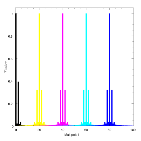
Figure 7: Sample band power window functions are shown for the cleanest of the sky regions from Figure 8, all normalized so that the maximum value is unity. The approximate lack of leakage from odd numbers of multipoles away results from the approximate parity symmetry of this region.

II.5 Blind analysis and the power spectrum matrix

We compute the power spectrum matrix ${\bf C}_{l}$ in practice using the method of Hivon ; a similar approach was used by the Boomerang Ruhl02 and WMAP hinshawpower03 teams. This simply consists of expanding the masked sky patch in question in spherical harmonics and then correcting for window function effects. Our only variation is that we do not invert the window matrix to obtain anticorrelated band power estimates with delta function window functions. Rather, we simply divide by the quadratic estimators by the area of the window $\delta{\bf T}_{\l}^{2}$ window functions, which asymptotes to the unbiased minimum variance estimators of cl on scales much smaller than the sky patch analyzed. An example of our window functions is shown in Figure 7.

As an example, Figure 9 shows the measured power spectrum for the V-band, the cleanest of WMAP’s frequency bands.

One fact worth emphasizing is that our weighting scheme of equation (12) is totally blind, assuming nothing whatsoever about the CMB power spectrum, the foregrounds, the WMAP detector noise or external templates. The only assumption is that the CMB spectrum is the blackbody that the WMAP team have modeled it as, so that the CMB contributes equally to all five channels — otherwise the vector ${\bf e}$ would be replaced by some other constant vector. We see that there is no need to model the CMB, the foregrounds or the noise, since all we need for computing the optimal weights is the total power spectrum matrix ${\bf C}_{l}$, containing the total contribution from CMB, foregrounds and noise combined — and this can be measured directly from the data.

We can decompose ${\bf C}_{l}$ as a sum of two terms,

$${\bf C}_{\l}={\bf C}_{\l}^{\rm junk}+{\bf C}_{\l}^{\rm cmb}={\bf C}_{\l}^{\rm junk}+C_{\l}^{\rm cmb}{\bf e}{\bf e}^{t},$$ (14)

where the second term is the CMB contribution and the first term is the contribution from noise and foregrounds. Note that if we keep ${\bf C}_{\l}^{\rm junk}$ fixed and change $C_{\l}^{\rm cmb}$, the weights given by equation (12) stay the same. The easiest way to see this is to note that the quantity we are minimizing is $\langle|a_{\ell m}|^{2}\rangle={\bf w}^{t}C_{\l}{\bf w}={\bf w}^{t}{\bf C}_{\l}^{\rm junk}{\bf w}+C_{\l}^{\rm cmb}({\bf e}\cdot{\bf w})^{2}={\bf w}^{t}{\bf C}_{\l}^{\rm junk}{\bf w}+C_{\l}^{\rm cmb}$, so the CMB power is just an additive constant that does not affect the optimal weighting. This means that our method is blind to assumptions about the underlying (ensemble-averaged) CMB power spectrum. Although we will return below in Section II.7 to the issue of how to determine what fraction of the power ${\bf C}_{\l}$ comes from each of the two terms in equation (14), it is important to remember that this affects only the physical interpretation, not our cleaning method and the maps we produce.

II.6 Subdividing the sky

To minimize the variance in our cleaned map, we should take advantage of all ways in which the unwanted signals (noise and foregrounds) differ from the CMB in their contribution to the covariance matrix ${\bf N}$ in equation (6). Above we exploited their different dependence on angular scale $\l$. Unlike the CMB, foregrounds are not an isotropic Gaussian random field. Rather, their variance differs dramatically between clean and dirty regions of the sky. It is therefore desirable to subdivide the sky into a set of regions of increasing cleanliness and perform the cleaning separately for each one wiener . One then expects our method described above to settle on more aggressive weights for the dirtier regions, where foregrounds are much more of a concern than noise. A second advantage of such a subdivision is that the frequency dependence of the foregrounds is likely to differ between very dirty and very clean regions, again resulting in different optimal weights. The WMAP team used the latter argument to motivate their subdivision of the sky into 12 regions, and convincingly demonstrated that foreground spectra indeed did vary across the sky, notably for synchrotron radiation where the spectrum was found to steepen towards increasing galactic latitudes.

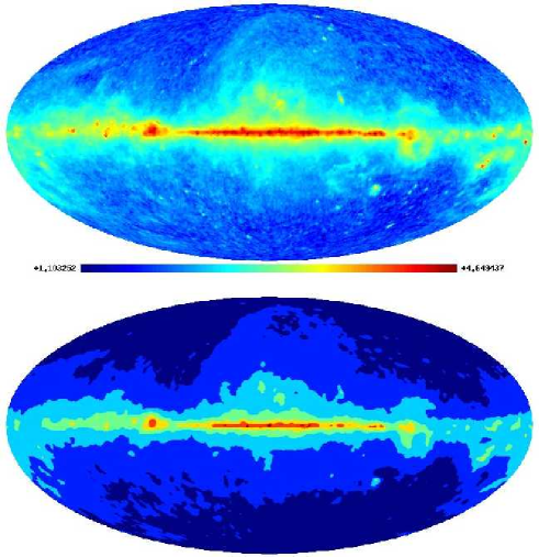
Figure 8: The top panel shows our junk map with a color scale that is uniform in the logarithm of the temperature in $\mu$K. The bottom panel show our subdivision of the sky into seven regions of decreasing cleanliness. From outside in, they correspond to junk map temperatures $T<100\mu{\rm K}$, $100\mu{\rm K}-300\mu{\rm K}$, $300\mu{\rm K}-1{\rm mK}$, $1{\rm mK}-3{\rm mK}$, $3{\rm mK}-10{\rm mK}$, $10{\rm mK}-30{\rm mK}$ and $T>30{\rm mK}$, respectively. The last of these regions contains only the set of roundish blobs in the inner Galactic plane. The second dirtiest region is seen to be topologically disconnected, and we treat its leftmost and rightmost blobs as separate regions, giving nine regions in total.

The WMAP team have created a set of sky-masks of increasing cleanliness based solely the K-band map. Although these masks are undoubtedly fine in practice, the procedure used in creating them is not blind, since it rests on the assumption that all dirty regions are dirty in the K-band. In particular, if a foreground manifests itself only at higher frequencies (imagine, say, a blob with localized dust emission without detectable synchrotron or free-free emission), it would go unnoticed. A second minor drawback of this K-band approach is that random CMB fluctuations affect the masks at a low level. In other words, the mask was based on the upper left map in Figure 2 which, as opposed to the upper right map, contains CMB fluctuations.

To preserve the blind nature of our method, we therefore create sky masks with a different procedure. We first form four difference maps W-V, V-Q, Q-K and K-Ka, thereby obtaining maps guaranteed to be free of CMB signal that pick up any signals with a non-CMB spectrum. We then form a combined “junk map” by taking the largest absolute value of these four maps at each point in the sky (Figure 8, top). Finally, we create disjoint sky regions based on contour plots of this map. We use cuts that are roughly equispaced on a logarithmic scale, corresponding to thresholds of 30000, 10000, 3000, 1000, 300 and 100$\mu$K (Figure 8, bottom). We emphasize that we have found no evidence whatsoever for any actual problems with the WMAP team masks, and opt to use our own simply to preserve the blind and CMB-independent nature of our analysis. As a cross-check, we also repeated our entire analysis using the WMAP masks Kp0, Lp2 and Kp12, obtaining similar results.

We followed the WMAP team procedure in the details of converting the contours into the masks shown in Figure 8 (bottom): we downsampled the junk map to HEALPpix resolution 64, imposed the cuts, went back up to HEALPix resolution 512, performed Gaussian smoothing with FWHM=$2^{\circ}$ on the $\{0,1\}$-valued mask and imposed a cutoff of 0.5. The WMAP team reported strong spatial variations of foreground spectra in the innermost parts of the galactic plane, and therefore subdivided this into 11 disjoint regions. We were unable to reproduce this procedure since they did not specify which these regions were. Instead, we merely lopped off three spatially disconnected islands in the two dirtiest regions as their own separate masks, as illustrated in Figure 8 (bottom), leaving 9 separate masks in total.

Our multipole-based cleaning is nonlocal in the spirit of equation (4), and although it guarantees that the CMB signal is preserved separately for each pixel, this is of course not the case for foregrounds. To avoid mirages of foreground emission from the Galactic plane leaking up to high latitudes, we clean the galaxy “from inside out”, i.e., clean the dirtiest region first, the second dirtiest region second, etc. To be specific, we start by defining five temporary maps, initially set equal to the five WMAP channels (Figure 2, left). We then repeat the following cleaning procedure nine times, once corresponding to each region $i=1,...,9$:

1. Compute the power spectrum matrix ${\bf C}_{\l}$ and the optimal weights ${\bf w}_{\l}$ for the $i^{th}$ region only.

2. Expand the five temporary maps in spherical harmonics and compute a cleaned all-sky map using the weights from step 1.

3. Replace the $i^{th}$ region of the temporary maps by the corresponding region in the cleaned map from step 2 (smoothed to the resolution appropriate for that channel, of course, by multiplying by $B_{\l}^{i}$ in $\l$-space).

Visually, one thus sees the foreground contamination gradually being cleaned off from Figure 2 as this iteration proceeds, starting in the inner Galactic plane and proceeding outward. At the end of the nine iterations, the five temporary maps equal the desired cleaned map at the K-, Ka-, Q-, V-, and W-band resolutions, respectively.

II.7 Interpretation of the cleaned maps

Figure 1 (bottom) shows our final cleaned map and Figure 10 shows its power spectrum in sky regions of varying cleanliness. We plot all maps after 21^′ Gaussian smoothing (giving a net FWHM of 24^′) to prevent them from being undersampled by the pixels in the image. The reader interested in using this map can download the corresponding 13 Megabyte HEALPix fits file from the web. To use this map, it is important to be clear on how to interpret it.

First of all, it is a sum of CMB, foreground and detector noise fluctuations. Although it was constructed by minimizing its power spectrum $C_{\l}^{\rm clean}={\bf w}_{\l}^{t}{\bf C}_{\l}{\bf w}_{\l}$, its power nonetheless gives a lower bound on the CMB power spectrum, since the minimization was performed subject to the constraint that the CMB be preserved; ${\bf e}\cdot{\bf w}=1$.

So what fraction of the power seen in Figure 10 is due to CMB, foregrounds and detector noise, respectively? Let us first get some rough estimates from the figures, then present more quantitative limits. Since this paper is focused on minimizing foregrounds, not on physically modeling them, the interested reader is referred to the detailed foreground study of the WMAP team BennettForegs for more information.

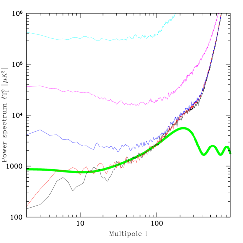
Figure 9: Total power spectra for CMB, foregrounds and noise combined are shown for the 61 GHz V-band, the one with the overall lowest foreground levels. This is the $(4,4)$ element of the power spectrum matrix ${\bf C}_{\l}$. From bottom to top, they correspond to the five cleanest sky regions shown in Figure 8. For comparison, the thick curve shows the best-fit CMB model from Spergel03 ; verde03 .

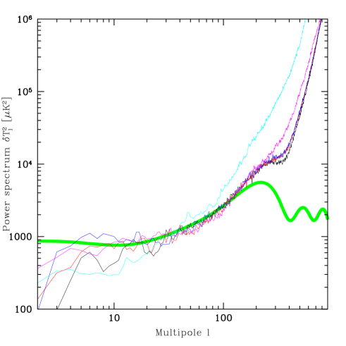
Figure 10: Same as previous figure, but for our foreground-cleaned CMB map (bottom panel of Figure 1). The power spectra of the cleanest sky regions are seen to be virtually identical with those for V-band on large scales, showing how subdominant smooth foregrounds are at 61 GHz.

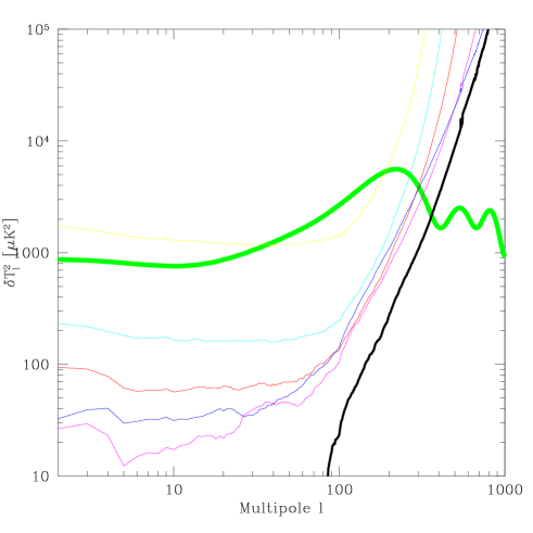
Figure 11: Power spectra of non-CMB signals (foregrounds plus detector noise) in the cleanest part of the sky shown in Figure 8. The five thin curves show the power spectra of five maps on the right side of Figure 2, i.e., the five WMAP channels after our cleaned CMB map (Figure 1, bottom) has been subtracted out. From top to bottom, the five curves correspond to 22.8, 33.0, 40.7, 93.5 and 60.8 GHz, respectively (note that the second highest frequency, V-band, is the cleanest). These curves should be interpreted as lower limits on foregrounds plus noise. The black curve gives the lower limit on foregrounds plus noise in our cleaned map using the method described in the text.

The WMAP team cleverly eliminated the average noise contribution by using only cross-correlations between different differencing assemblies (DAs) to measure the power spectrum, and used a combination of sky cutting and foreground subtraction (with external templates) to minimize the foreground contribution. The best fit cosmological model Spergel03 ; verde03 to their measured CMB power spectrum hinshawpower03 is shown for comparison in figures 9 and 10. For $\l\mathrel{\hbox to0.0pt{\lower 3.0pt\hbox{$\mathchar 536\relax$}\hss}\raise 2.0pt\hbox{$\mathchar 316\relax$}}100$, it is seen to agree well with the lower envelope of our curves in Figure 9, suggesting that foregrounds are subdominant in the cleanest parts of the 61 GHz sky. Figure 10 shows no noticeable excess power at $\l\l\mathrel{\hbox to0.0pt{\lower 3.0pt\hbox{$\mathchar 536\relax$}\hss}\raise 2.0pt\hbox{$\mathchar 316\relax$}}100$ due to foregrounds in the cleaned map in any of the four cleanest sky regions from Figure 8, which together cover all but the very innermost Galactic plane.

The slight power deficit on the very largest scales has two causes: one is the low quadrupole, to which we return in Section III below, which pulls down neighboring band power estimates because the band-power window, illustrated in Figure 7, contains small off-diagonal contributions. The second cause is that we have not corrected for the effects of monopole and dipole removal, which pulls down the power estimates on the scale of the sky patch in question (our method produces an unbiased CMB map regardless of what ${\bf C}_{\l}$ we use in equation (12), so this merely raises the variance in the cleaned map above the optimal level). On smaller scales, detector noise starts to dominate, and is seen to push our curves way above the CMB curve. A worthwhile future project for further quantifying foregrounds would be to repeat our analysis with ${\bf C}_{\l}$ estimated in a way that removes the detector noise contribution. For Q, V and W bands, which each have more than one DA, this can be done using cross-correlations. For the $(1,1)$ and $(2,2)$ components of ${\bf C}_{\l}$ (the K and Ka power spectra), it would involve subtracting the noise power using the WMAP team’s noise model.

We can, however, give some quantitative limits even based on our measured ${\bf C}_{\l}$ alone. Grouping the five coefficients $a_{\ell m}^{i}$ into a five-dimensional vector ${\bf a}_{\l m}$, equation (13) becomes simply ${\bf C}_{\l}=\langle{\bf a}_{\l m}^{*}{\bf a}_{\l m}^{t}\rangle$, and the cleaned procedure can be written $a_{\ell m}={\bf w}\cdot{\bf a}_{\l m}$. Using equation (12) shows that the power in the cleaned map is

$$C_{\l}^{\rm clean}={1\over{\bf e}^{t}{\bf C}_{\l}^{-1}{\bf e}}.$$ (15)

By subtracting our cleaned map from the input map, we obtain maps showing in Figure 2 (right). These are guaranteed to be free from CMB power, since the cleaned map gave a lower limit on the CMB. Most likely, we have subtracted some foreground power too, so the five maps should be interpreted as placing lower limits on the foreground power. (As a toy example, imagine synchrotron, free-free and dust emission tracing each other perfectly; the sum of their three spectra can then be written as a constant, which our method will interpret as CMB, plus a non-negative residual, which our method will interpret as foregrounds). Using equation (14), the covariance matrix of these five CMB-free “junk maps” is

$${\bf C}_{\l}^{\rm junk}\geq{\bf C}_{\l}^{\rm nocmb}\equiv{\bf C}_{\l}-C_{\l}^{\rm clean}{\bf e}{\bf e}^{t}={\bf\Pi}_{\l}{\bf C}_{\l}{\bf\Pi}_{\l}^{t},$$ (16)

where the projection matrix

$${\bf\Pi}_{\l}\equiv{\bf I}-{\bf e}{\bf w}_{\l}^{t}$$ (17)

satisfies ${\bf\Pi}_{\l}^{2}={\bf\Pi}_{\l}$, ${\bf\Pi}_{\l}{\bf e}=0$ and ${\bf\Pi}_{\l}^{t}{\bf w}=0$ and can be interpreted as projecting out the CMB component. In this notation, the maps in Figure 2 (right) are defined by simply ${\bf\Pi}_{\l}{\bf a}_{\l m}$. The inequality ${\bf C}_{\l}^{\rm junk}\geq{\bf C}_{\l}^{\rm nocmb}$ refers only to the diagonal elements of these matrices. The five diagonal elements of ${\bf C}_{\l}^{\rm junk}$ are plotted in Figure 11 for our cleanest sky region from Figure 8.

How much of ${\bf C}_{\l}$ can possibly be due to CMB? In other words, forgetting for a moment about the weighting that gave equation (15), how large can we make $C_{\l}^{\rm cmb}$ in equation (16) before the covariance matrix ${\bf C}_{\l}^{\rm junk}$ gets unphysical properties? First of all, no covariance matrix can have negative eigenvalues, so we we must stop increasing $C_{\l}^{\rm cmb}$ once the smallest eigenvalue of ${\bf C}_{\l}^{\rm junk}$ drops to zero. In fact, ${\bf\Pi}^{t}{\bf w}=0$ implies that when using our optimal weighting and hence equation (15), ${\bf C}_{\l}^{\rm junk}$ has a vanishing eigenvalue corresponding to the vector ${\bf w}$, and it is easy to show that this alternative method for estimating $C_{\l}^{\rm cmb}$ is equivalent to our original method, being simply an alternative derivation of equation (15).

Let us now make a second assumption: that ${\bf C}_{\l}^{\rm junk}$ cannot have any negative elements. The noise covariance matrix is guaranteed to have this property, since the absence of correlations between bands implies that it is diagonal. The foreground covariance matrix is also guaranteed to have this property if foreground emission is indeed emission, i.e., if foregrounds can make only positive contributions to the sky maps. Pure absorption at all frequencies likewise give only positive correlations. This assumption, made also in the Maximum-Entropy analysis of BennettForegs is likely to be valid WMAP frequencies, since the only known exception is the thermal SZ effect, and it changes sign only outside of the WMAP frequency range (around 217 GHz). In summary, we therefore have two separate limits on the CMB power spectrum:

$$C_{\l}^{\rm cmb} \leq C_{\l}^{\rm clean},$$ (18)

$$C_{\l}^{\rm cmb} \leq \min_{i,j}({\bf C}_{\l})_{ij}.$$ (19)

$C_{\l}^{\rm clean}$ is also the actual variance of the cleaned map, so if the second limit is lower than first, then we know that the difference cannot be due to CMB.

To gain intuition, consider the following two examples of the junk + CMB decomposition of equation (14) for the simple case of only two frequency bands:

$${\bf C}_{\l}=\left(\begin{tabular}[]{cc}5&3\\ 3&2\end{tabular}\right) = \left(\begin{tabular}[]{cc}4&2\\ 2&1\end{tabular}\right)+\left(\begin{tabular}[]{cc}1&1\\ 1&1\end{tabular}\right)$$ (26)

$${\bf C}_{\l}=\left(\begin{tabular}[]{cc}2&1\\ 1&2\end{tabular}\right) = {1\over 2}\left(\begin{tabular}[]{cc}1&-1\\ -1&1\end{tabular}\right)+{3\over 2}\left(\begin{tabular}[]{cc}1&1\\ 1&1\end{tabular}\right)$$ (33)

$$= \left(\begin{tabular}[]{cc}1&0\\ 0&1\end{tabular}\right)+\left(\begin{tabular}[]{cc}1&1\\ 1&1\end{tabular}\right)$$ (38)

In the first case, equation (15) gives $C_{\l}^{\rm cmb}=1$, i.e., the largest contribution we can possible attribute to the CMB (the second term) is ${\bf e}{\bf e}^{t}$ — if we scaled up the last term, then ${\bf C}_{\l}^{\rm junk}$ (the first term) would acquire an unphysical negative eigenvalue. Moreover, we see that ${\bf C}_{\l}^{\rm junk}$ looks like the covariance matrix of a perfectly respectable foreground, with a spectrum such that it contributes twice as high rms fluctuations to the first channel as to the second, and with perfect correlation between the two (the dimensionless correlation coefficient is $r=1$). Such a foreground would be completely removed by our method, and so we cannot place any lower limit on the foreground contribution to the cleaned map in this case. In the second case, equation (15) gives $C_{\l}^{\rm cmb}=3/2$, so this will be the variance in the cleaned map. However, ${\bf C}_{\l}^{\rm junk}$ (the first term) in equation (33) exhibits an unphysical anticorrelation between the two bands which neither noise nor foregrounds could produce, and equation (19) tells us that the CMB power $C_{\l}^{\rm cmb}\leq 1$, corresponding to the alternative decomposition on the last line. This means that the junk map must have a power contribution of at least $1/2$ which is not due to CMB.

This difference, which places a lower limit on the amount of non-CMB signal in our cleaned map, is shown as the black line in Figure 11 for our actual five-band case. We see that although we get an interesting lower limit for $\l>100$, presumably dominated by detector noise, the residual foreground level is consistent with zero at low $\l$.

II.8 Wiener filtering

Figure 1 (bottom) shows our cleaned map of the CMB sky, and this is the map that should be used for cross-correlation analysis with other data sets and other scientific applications. For visualization purposes, however, we can do better. The “best-guess” map of what the CMB looks like, in the sense of minimizing the rms errors, is the Wiener filtered map defined by Wiener49

$$a_{\ell m}^{\rm Wiener}={C_{\l}^{\rm cmb}\over C_{\l}^{\rm clean}}a_{\ell m}.$$ (39)

This staple signal processing technique, multiplying by “signal over signal plus noise”, has additional attractive properties; for instance, it constitutes the best-guess (maximum posterior probability) map in the approximation of Gaussian fluctuations. Examples of recent applications of Wiener filtering to CMB and galaxy mapping include Rybicki92 ; Lahav94 ; Fisher95 ; Zaroubi95 ; Bond95 ; Bunn96 ; saskmap . Our resulting Wiener filtered map is shown in Figure 1 (middle), using the best fit model from the WMAP team Spergel03 ; verde03 as our estimate of $C_{\l}^{\rm cmb}$ in the numerator of equation (39). For the denominator, we take the larger of our measured $C_{\l}^{\rm clean}$ and $C_{\l}^{\rm cmb}$, so that the ratio is guaranteed to be $\leq 1$. The result is not an unbiased CMB map. Rather, equation (39) shows that each multipole gets multiplied by a number between 0 and 1, so features with high signal-to-noise are left unaffected whereas features that are not statistically significant become suppressed. This means that the features that you see in Figure 1 (middle) are likely to be real CMB fluctuations, having signal-to-noise exceeding unity.

The cleaned map at the bottom of Figure 1 reveals some residual galactic fluctuations on very small angular scales, caused mainly by the fact that no other channels have fine enough angular resolution to help clean the W-band map for very large $\l$. We Wiener filter each of the nine sky regions from Figure 8 separately, so $C_{\l}^{\rm clean}$ is much higher near the Galactic plane. This is why the Galactic contamination is imperceptible in the Wiener filtered map: equation (39) automatically suppresses fluctuations in regions with large residual foregrounds.

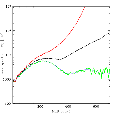
Figure 12: Comparison of the total (CMB+foregrounds+noise) power spectra of the WMAP team internal linear combination map BennettForegs (top curve) and our cleaned map (middle curve), both for our cleanest sky region. Both of these cleaned maps are seen to reproduce on large scales the CMB power spectrum measured by the WMAP team hinshawpower03 (lower wiggly curve), which has no net noise contribution because it is based on cross-correlations between channels. The lower smooth curve is the WMAP team’s best fit model Spergel03 ; verde03 . As explained in the text, the noise contribution is seen to become important earlier in the WMAP team’s cleaned map than in ours because it is limited by the lowest resolution frequency bands. All power spectra have been smoothed with a boxchar filter of width $\Delta\l=10$ to reduce scatter.

III Discussion

We have performed an independent foreground analysis of the WMAP maps to produce a cleaned CMB map. The only assumption underlying our method is that the CMB contributes equally to all five channels. This assumption rests on very solid ground BennettWMAP . The basic reason for this is that the COBE/FIRAS determination of the CMB spectrum Mather94 is based on the absolute CMB signal, which is about $10^{5}$ times larger than the fluctuations that we have considered in this paper.

Figure 1 shows that our map agrees very well with the internal linear combination (ILC) map from the WMAP team on the scales $\mathrel{\hbox to0.0pt{\lower 3.0pt\hbox{$\mathchar 536\relax$}\hss}\raise 2.0pt\hbox{$\mathchar 318\relax$}}1^{\circ}$ where they can be compared. This is yet another testimony to the high signal-to-noise in the WMAP data and to the fact that unpolarized CMB foregrounds are manageable: the basic spatial features of the CMB are insensitive to the details of the foreground removal method used.

The basic advantage of our map is illustrated in Figure 12, which compares its all-sky power spectrum with that of the WMAP team ILC map. Both power spectra have had beam effects removed here; in Figure 1, our map is shown at the W-band resolution and the ILC map is shown at $1^{\circ}$ resolution as released.

The first thing to note from Figure 12 is that foregrounds appear highly subdominant in both maps, since their power spectra essentially coincide with the WMAP CMB power spectrum on large scales where noise becomes unimportant. Second, as expected, the main improvement in our map is seen to be on the smaller scales where noise is important, gaining a factor of 30% at the first acoustic peak and about a factor of two at the second peak where noise from the low frequency channels is beginning to exponentially dominate the ILC map.

We hope that our map will prove useful for a variety of scientific applications. For cross-correlation with external maps, its lowered noise power should be particularly advantageous for pulling out small-scale signals, for instance those associated with lensing and SZ clusters. Rather that attempting detailed modeling of the residual noise and foreground fluctuations in our map, a simple way to place error bars on such correlations will be repeating the analysis with a suite of rotated and flipped versions of our map as in, e.g., 19ghz .

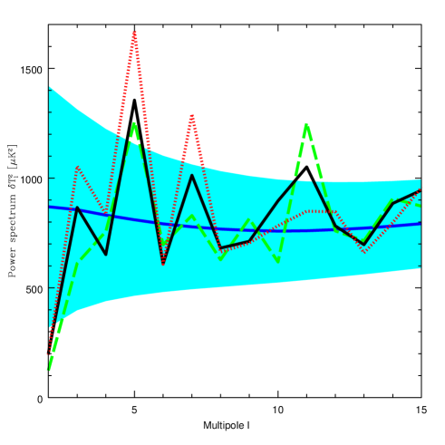
Figure 13: A heretic all-sky analysis of our cleaned map (solid jagged curve) gives a slightly less low quadrupole $\delta T_{2}^{2}$ than the cut-sky WMAP analysis hinshawpower03 (dashed curve), and also agrees well with the quadrupole from an all-sky analysis of the WMAP team cleaned map of BennettForegs (dotted curve). The smooth curve shows the WMAP team best fit model Spergel03 ; verde03 with the band indicating the cosmic variance errors (WMAP noise and beam effects are completely negligible on these scales).

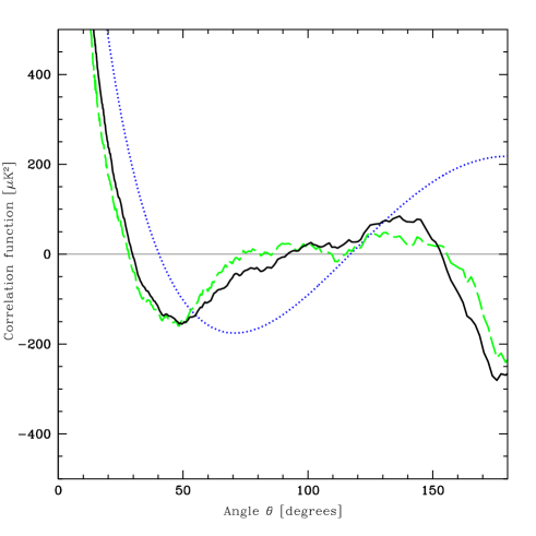
Figure 14: The angular correlation functions are shown corresponding to our all-sky cleaned map (solid curve), the cut-sky WMAP power spectrum (dashed curve) and the best-fit WMAP team cosmological model (dotted curve). This is simply the Legendre transform of the power spectra from the previous figure, i.e., $(4\pi)^{-1}\sum_{\l}(2\l+1)P_{\l}(\cos\theta)C_{\l}$, so the the quadrupole and octopole contributions are shaped as $3\cos^{2}\theta-1$ and $5\cos^{3}\theta-3\cos x$, respectively.

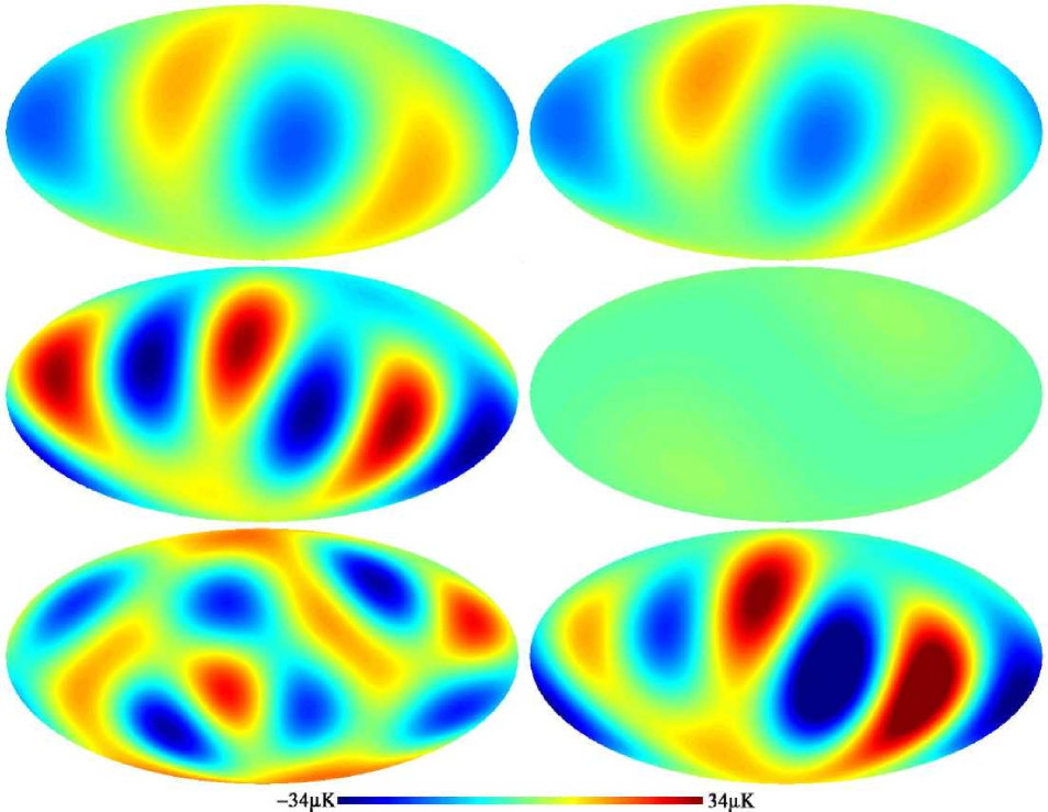
Figure 15: The left panel shows the quadrupole (top), octopole (middle) and hexadecapole (bottom) components of our cleaned all-sky CMB map from Figure 1 on a common temperature scale. Note that not only is the quadrupole power low, but both it and the octopole have almost all their power perpendicular to a common axis in space, as if some process has suppressed large-scale power in the direction of this axis. We computed the corresponding images for the WMAP team ILC map as well, and found them to be very similar. The right panel shows he cosmic quadrupole (top) after a correcting for a crude estimate of the dynamic quadrupole (middle) from our motion relative to the CMB rest frame. The bottom right map shows the sum of the quadrupole and octopole maps from the left panel.

Table 1 – Measurements of the CMB quadrupole and octopole.

Measurement	$\delta T_{2}^{2}$ $[\mu$K${}^{2}]$	p-value	$\delta T_{3}^{2}$ $[\mu$K${}^{2}]$
Spergel et al. model	869.7		855.6
Hinshaw et al. cut sky	123.4	1.8%	611.8
ILC map all sky	195.1	4.8%	1053.4
Cleaned map all sky	201.6	5.1%	866.1
Cosmic quadrupole	194.2	4.7%
Dynamic quadrupole	3.6

Let us close by returning from small to large angular scales. The surprisingly small CMB quadrupole has intrigued the cosmology community ever since if was first observed by COBE/DMR Smoot92 , and simulations by Spergel03 ; verde03 show that the low value observed by WMAP is sufficiently unlikely to warrant serious concern. The WMAP team measured the quadrupole using only the part of the sky outside of their Galactic cut, and stress that the dominant uncertainty in its value is foreground modeling. While we agree with this assessment, it should be borne in mind that noise variance and beam issues are completely negligible on these huge angular scales, so this does not imply that the foreground uncertainties are large compared to the signal itself. Indeed, Figure 12 suggests that foregrounds are subdominant to the intrinsic CMB signal even without any Galaxy cut if a foreground-cleaned map is used. While the reader may feel disturbed by the clearly visible Galactic residuals in Figure 1 (in both the top and bottom maps), it is important to bear in mind that these signals are present in only a tiny fraction of the total sky area and therefore contribute little to the total power spectrum.

To quantify the impact of the Galactic plane, we computed a sequence of all-sky power spectra for both our map and the ILC map. We first used the unadulterated maps, then repeated the calculation after repacing the dirtiest of the nine regions from Figure 8 with zeroes, then zeroed our the 2nd dirtiest region as well, etc. This zeroing procedure obviously biases the measurements by removing power, by an amount related to the zeroed area, but provides a powerful test of how sensitive the results are to Galactic plane details. We also band-pass filtered the resulting maps to produce spatial plots of the quadrupole, octopole and hexadacapole. We found that zeroing out the dirtiest parts of the Galactic plane had a negligible effect on both the power spectrum and on the spatial structure of these lowest multipoles. Specifically, we could zero out all but the three cleanest regions Figure 8 (everything with $T>1$mK) without the quadrupole or octopole changing substantially. The spatial morphology of the quadrupole, octopole and hexadecapole for the all-sky analysis agrees well between our map and the ILC map, again showing insensitivity to galaxy modeling details (in particular, the ILC map is likely to have less contamination in the Galactic plane due to more subdivisions there).

Although more detailed foreground modeling would be needed to rigorously quantify the foreground contribution to low multipoles, let us, encouraged by the above-mentioned tests, tentatively assume that this contribution is unimportant and perform an all-sky analysis of our cleaned map. The resulting power spectrum is shown in Figure 13, which is simply a blow-up of the leftmost part of the previous figure, and the corresponding angular correlation function is shown in Figure 14.

Table 1 summarizes the quadrupole and octopole results. We see that although the quadrupole is still low, it is not quite as low as that from the cut-sky WMAP team analysis of hinshawpower03 . Moreover, our map has a quadrupole virtually identical to the WMAP team ILC map despite the differences in foreground modeling, further supporting our hypothesis that the quadrupole is not strongly affected by foregrounds. The second column in Table 1 shows the probability of the quadrupole in our Hubble volume being as low as observed if the best-fit WMAP team model from Spergel03 ; verde03 is correct. This is computed for the all-sky case where $\delta T^{2}_{2}$ has a $\chi^{2}$-distribution with 5 degrees of freedom, so the probability tabulated is simply $1-\gamma[5/2,(5/2)T^{2}_{2}/855.6\mu{\rm K}^{2}]/\Gamma(5/2)$, where $\gamma$ and $\Gamma$ are the incomplete and complete Gamma functions, respectively. We see that the statistical significance of the low quadrupole problem drops substantially with our all-sky analysis, below the 95% significance level, requiring merely a one-in-twenty fluke.

To understand why the all-sky quadrupole is larger than the cut-sky one measured by the WMAP team, we plot the lowest three multipoles of our cleaned map in Figure 15, all on the same temperature scale. Several features are noteworthy. First of all, the quadrupole is low with an interesting alignment. A generic quadrupole has three orthogonal pairs of extrema (two maxima, two minima and two saddle points). We see that the actual CMB quadrupole has its strongest pair of lobes, apparently coincidentally, fall near the Galactic plane. Applying a Galaxy cut therefore removes a substantial fraction of the quadrupole power. The saddle point is seen to be close to zero. In other words, there is a preferred axis in space along which the observed quadrupole has almost no power.

Second, the observed quadrupole is the sum of the cosmic quadrupole and the dynamic quadrupole due to our motion relative to the CMB rest frame - see KamionKnox02 for a detailed discussion. Since this motion is accurately known from the CMB dipole measurement Smoot92 ; BennettWMAP , the dynamic quadrupole can and should be subtracted when studying the cosmic contribution. Figure 15 shows the dynamic quadrupole approximated by $(v/c)^{2}(\cos\theta^{2}-1/3)$, where $v\approx 369km/s$ towards $(l,b)\approx(264,48)$ is the velocity of the Solar System relative to the CMB BennettWMAP and $\theta$ is the angle relative to this velocity vector. This is a small correction with peak-to-peak amplitude $(v/c)^{2}\sim 4\mu{\rm K}$, and Table 1 shows that it reduces the cosmic quadrupole slightly. This approximation is crude since the dynamic quadrupole in fact depends on frequency KamionKnox02 , and therefore may have been either over- or under-estimated in our foreground cleaned map - we have shown it here merely to illustrate its spatial orientation and give an order-of-magnitude estimate of its importance.

Third, although the overall octopole power is large, not suppressed like the quadrupole, it too displays the unusual property of a preferred axis along which power is suppressed. Moreover, this axis is seen to be approximately aligned with that for the quadrupole. The reason that our measured octopole in Figure 13 is larger than that reported by the WMAP team is therefore, once again, that much of the power falls within the Galaxy cut. In contrast, the hexadecapole is seen to exhibit the more generic behavior we expect of an isotropic random field, with no obvious preferred axis.

How significant is this quadrupole-octopole alignment? As a simple definition of preferred axis for an arbitrary sky map, smalluniverse computes the unit vector $\widehat{{\bf r}}$ around which the angular momentum dispersion $\langle(\widehat{{\bf r}}\cdot\L)^{2}\rangle=\sum_{m}m^{2}|a_{\l m}(\widehat{{\bf r}})|^{2}$ is maximized. Here $a_{\l m}(\widehat{{\bf r}})$ denotes the spherical harmonic coefficients of the map in a rotated coordinate system with its $z$-axis in the the $\widehat{{\bf r}}$-direction. The preferred axes $\widehat{{\bf r}}_{2}$ and $\widehat{{\bf r}}_{3}$ for the quadrupole and octopole, respectively, are

$$\widehat{{\bf r}}_{2} = (-0.1145,-0.5265,0.8424),$$

$$\widehat{{\bf r}}_{3} = (-0.2578,-0.4207,0.8698),$$ (40)

i.e., both roughly in the direction of $(l,b)\sim(-110^{\circ},60^{\circ})$ in Virgo. The angle between these two axes is merely $10.3^{\circ}$, and the probability that a random axis falls inside a circle of radius $10.3^{\circ}$ around the quadrupole axis is simply the area of this circle over the area of the half-sphere, about $1/62$. In other words, if the CMB is an isotropic Gaussian random field, then a chance alignment this good requires about a 1-in-62 fluke. This issue is discussed in greater detail in smalluniverse .

What does this all mean? Although we have presented these low multipole results merely in an exploratory spirit, and more thorough modeling of the foreground contribution to $\l=2$ and $\l=3$ is certainly warranted, it is difficult not to be intrigued by the similarities of Figure 13 with what is expected in some non-standard models, for instance ones involving a flat “small Universe” with a compact topology as in Starobinsky ; Stevens ; bb1 ; bb2 ; Levin01 ; Rocha and one of the three dimensions being relatively small (of order the Horizon size or smaller). This could have the effect of suppressing the large-scale power in this particular spatial direction in the same sense as is seen in Figure 13. As so often in science when measurements are improved, WMAP has answered old questions and raised new ones.

We thank the the WMAP team for producing such a superb data set and for promptly making it public via the Legacy Archive for Microwave Background Data Analysis (LAMBDA). Support for LAMBDA is provided by the NASA Office of Space Science. We thank Krzysztof Górski and collaborators for creating the HEALPix package healpix1 ; healpix2 , which we used both for harmonic transforms and map plotting. Thanks to Ed Bertschinger, Gary Hinshaw, Jim Peebles, Ned Wright and Matias Zaldarriaga for helpful comments. This work was supported by NSF grants AST-0071213, AST-0134999, & AST-0205981, and by NASA grants NAG5-10763 & NAG5-11099. MT was supported by a David and Lucile Packard Foundation fellowship and a Cottrell Scholarship from Research Corporation.

References

- (1) C. L. Bennett et al., astro-ph/0302207 (2003).
- (2) C. L. Bennett et al., astro-ph/0301158 (2003).
- (3) C. L. Bennett et al., astro-ph/0302208 (2003).
- (4) C. Barnes et al., astro-ph/0301159 (2003).
- (5) C. Barnes et al., astro-ph/0302215 (2003).
- (6) G. Hinshaw et al., astro-ph/0302217 (2003).
- (7) G. Hinshaw et al., astro-ph/0302222 (2003).
- (8) N. Jarosik et al., astro-ph/0301164 (2003).
- (9) N. Jarosik et al., astro-ph/0302224 (2003).
- (10) A. Kogut et al., astro-ph/0302213 (2003).
- (11) E. Komatsu et al., astro-ph/0302223 (2003).
- (12) M. Limon et al., astro-ph/ (2003).
- (13) L. Page et al., astro-ph/0301160 (2003).
- (14) L. Page et al., astro-ph/0302214 (2003).
- (15) L. Page et al., astro-ph/0302220 (2003).
- (16) H. V. Peiris et al., astro-ph/0302225 (2003).
- (17) D. N. Spergel et al., astro-ph/0302209 (2003).
- (18) L. Verde et al., astro-ph/0302218 (2003).
- (19) H. V. Peiris and D. N. Spergel, ApJ 540, 605 (2000).
- (20) S. P. Boughn R. G. Crittenden, and G. Koehrsen P, ApJ 580, 672 (2002).
- (21) J. Diego M, and J. Silk, astro-ph/0302268 (2003).
- (22) Y. S. Song A. Cooray L. Knox, and M. Zaldarriaga, ApJ 590, 664 (2002).
- (23) A. Cooray, PRD 65, 103510 (2002).
- (24) C. M. Hirata and U. Seljak, PRD 67, 043001 (2003).
- (25) Z. Haiman, and G. P. Holder, astro-ph/0302403 (2003).
- (26) G. Holder Z. Haiman M. Kaplinghat, and L. Knox, astro-ph/0302404 (2003).
- (27) L. Hui, and Z. Haiman, astro-ph/0302439 (2003).
- (28) M. Tegmark, and G. Efstathiou, MNRAS 281, 1297 (1996).
- (29) M. Tegmark, D. J. Eisenstein, W. Hu, and A. de Oliveira-Costa, ApJ 530, 133 (2000).
- (30) A. de Oliveira-Costa et al., astro-ph/0212419 (2002).
- (31) A. de Oliveira-Costa, and M. Tegmark (Ed.), ASP (1999).Conf.Ser., Microwave Foregrounds (San Francisco: ASP)
- (32) A. de Oliveira-Costa et al., ApJ 567, 363 (2002).
- (33) F. R. Bouchet et al., Space Science Rev. 74, 37 (1995).
- (34) F. R. Bouchet and R. Gispert, New Astron. 4, 443 (1999).
- (35) F. R. Bouchet, R. Gispert, and J. L. Puget 1996, in Unveiling the Cosmic Infrared Background, ed. E. Dwek (AIP: Baltimore;255)F. R. Bouchet, S. Prunet, and S. K. Sethi, MNRAS 302, 663 (1999).
- (36) M. Tucci, E. Carretti, S. Cecchini, R. Fabbri, M. Orsini, and E. Pierpaoli, New Astr 5, 181 (2000).
- (37) C. Baccigalupi, C. Burigana, Perrotta F, G. De Zotti, L. La Porta, D. Maino, M. Maris, and R. Paladini, A&A 372, 8 (2001).
- (38) C. Burigana, and L. La Porta, astro-ph/0202439 (2002).
- (39) M. Bruscoli, M. Tucci, V. Natale, E. Carretti, R. Fabbri, C. Sbarra, and S. Cortiglioni, New Astr 7, 171 (2002).
- (40) M. Tucci, E. Carretti, S. Cecchini, L. Nicastro, R. Fabbri, B. M. Gaensler, J. M. Dickey, and N. M. McClure-Griffiths, ApJ 579, 607 (2002).
- (41) G. Giardino, A. J. Banday, K. M. Gorski, K. Bennett, J. L. Jonas, and J. Tauber, A&A 387, 82 (2002).
- (42) K. M. Górski, E. Hivon, and B. D. Wandelt 1999; astro-ph/9812350, in Evolution of Large-Scale Structure, ed. A. J. Banday, R. S. Sheth, and L. (. da CostaPrintPartners Ipskamp: Nethernalds), p37
- (43) K. M. Górski, B. D. Wandelt, Hansen F K, and A. Banday J, astro-ph/9905275 (1999).
- (44) E. L. Wright et al., astro-ph/9601059 (1996).
- (45) M. Tegmark, ApJL 480, L87 (1997).
- (46) P. F. P. Natoli.. Muciaccia,, and N. Vittorio, ApJ 488, 63 (1997).
- (47) L. Knox, Phys. Rev. D 48, 3502 (1995).
- (48) M. Tegmark, ApJ 502, 1 (1998).
- (49) E. Hivon, K. M. Górski, C. B. Netterfield, B. P. Crill, S. Prunet, and F. Hansen, ApJ 567, 2 (2002).
- (50) J. E. Ruhl, astro-ph/0212229 (2002).
- (51) M. Tegmark, Phys. Rev. D 55, 5895 (1997).
- (52) N. Wiener, Extrapolation and Smoothing of Stationary Time Series (Wiley, New York, 1949).
- (53) G. B. Rybicki and W. H. Press, ApJ 398, 169 (1992).
- (54) O. Lahav et al., ApJ 423, L93 (1994).
- (55) K. B. Fisher et al., MNRAS 272, 885 (1995).
- (56) S. Zaroubi et al., ApJ 449, 446 (1995).
- (57) J. R. Bond, Phys. Rev. Lett. 74, 4369 (1995).
- (58) E. F. Bunn, Y. Hoffmann, and J. Silk, ApJ 464, 1 (1996).
- (59) M. Tegmark et al., ApJL 474, L77 (1996).
- (60) J. Mather et al., ApJ 420, 439 (1994).
- (61) A. de Oliveira-Costa et al., ApJL 509, L9 (1998).
- (62) G. F. Smoot et al., ApJ 396, L1 (1992).
- (63) M. Kamionkowski and L. Knox, PRD;67;063001 (2003).
- (64) A. de Oliveira-Costa, M. Tegmark, M. Zaldarriaga, and A. J. S Hamilton, astro-ph/0307282 (2003).
- (65) n. n. Starobinsky, JETP Lett. 57, 622 (1993).
- (66) D. Stevens, D. Scott, and J. Silk, PRL 71, 20 (1993).
- (67) A. de Oliveira-Costa and G. F. Smoot, ApJ 448, 477 (1995).
- (68) A. de Oliveira-Costa, G. F. Smoot, and A. A. Starobinski, ApJ 468, 457 (1996).
- (69) J. Levin, Phys. Rep. 365, 251 (2002).
- (70) G. Rocha et al., astro-ph/0205155 (2002).