Studying clusters with Planck

Abstract

We use mock Sunyaev-Zel’dovich effect (SZE) maps to investigate how well the Planck mission might find and characterize clusters of galaxies. We discuss different combinations of frequency maps and different methods for identifying cluster candidates. For the simplest methods, the catalogues are not complete even for relatively high mass thresholds, but the full sky nature of the mission ensures a large sample of massive, high-$z$ clusters which will be ideal for many studies. We make a preliminary attempt to identify the X-ray, optical and weak lensing properties of the Planck sample.

1. Introduction

The Planck mission will provide all-sky maps of superb resolution at 9 frequencies, ranging from $30\,$GHz to $850\,$GHz, with unprecedented signal-to-noise. One of the science goals that this enables is the construction of a catalogue of galaxy clusters detected through the Sunyaev-Zel’dovich effect (SZE: Sunyaev & Zel’dovich (SZ72 (1972, 1980)); for recent reviews see Rephaeli Rep (1995) and Birkinshaw Bir (1999)) and a study of the residual SZ emission once these clusters are removed. In this paper we investigate some of the ways a survey with the characteristics of the Planck survey will advance our understanding of cluster physics and cosmology, building on the earlier work of many authors (Aghanim et al. Aghanim (1997); Kay, Liddle & Thomas KayLidTho (2001); Vielva et al. VBHMLST (2001); Herranz et al. HSHBDML (2002); Diego et al. Diego (2003); Hobson & McLachlan HobMcL (2003)). We discuss the sample Planck will select, what observations it can give of previously known clusters, and some of the properties of the clusters which will be useful for followup.

Exploring the expected Planck sample is a complex problem, involving several different but interlocking facets. Our aim here is to focus on one, while treating the others in as simple a manner as is consistent with what we know. This investigation is thus by nature preliminary, but we believe that the simulations upon which it is based provide an advance over what has been used in the past and illuminate several issues future Planck work will need to address. We use mock SZ maps drawn from a large volume, high resolution N-body simulation. These maps capture much of the physics behind the SZ effect, with the sources (groups and clusters) situated correctly in their cosmological context. Due to the current uncertainty in the amplitude of both the SZ signal and the relevant astrophysical foregrounds, a detailed modeling of the ‘noise’ is not possible. However we shall investigate signal-to-noise levels which should span the allowed range. Our investigations lead us to conclude that constructing a catalogue of clusters from Planck will be a difficult undertaking, but one which is worth a great deal of effort. Which are the optimal methods for foreground subtraction, cluster finding and modeling the selection function are all open questions currently, and this work will only begin to explore some of the relevant issues. Also uncertain is the most efficient way of collecting relevant information during the pre-launch phase of Planck.

The outline of the paper is as follows. In §2 we describe our methodology for isolating the SZ signal from the other astrophysical components (including the CMB) in our simulated observations, and the simulations we are using to model the SZ effect itself. We describe two methods for finding cluster candidates in our simulated maps in §3 and how well they do in §4. We discuss using the lower frequency channels of Planck in order to reduce IR point source contamination in §5. In §6 we describe the properties of our cluster sample from the point of view of X-ray, optical and weak lensing followup. The dependence of our results on our cosmological and foreground modeling is discussed in §7 and our conclusions are presented in §8.

2. Simulated observations

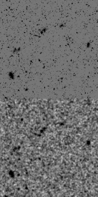
Figure 1.— One of our simulated maps: $\Delta T(353)-\Delta T(217)$. (Top) the input SZ signal, converted to $\Delta T$ at $353\,$GHz but without noise or smoothing. (Bottom) the same map, with $40\,\mu$K of noise and $5^{\prime}$ smoothing. In both panels the greyscale is linear in $\Delta T$ ranging from $-100\,\mu$K (white) to $+100\,\mu$K (black).

The thermal SZE signal is likely to be dominated by virialized objects whose typical angular size is around $1^{\prime}$. Thus if we can achieve a suitably low noise level, including foreground subtraction, the Planck channels which will be best suited to studying the SZE signal from galaxy clusters will be those at higher frequency, where the angular resolution is best. If it turns out that high frequency foregrounds are particularly troublesome, and cannot be removed to a suitable level, we may need to consider moving to lower frequencies, and resolutions, where the ‘noise’ is lower. We shall consider both approaches here, beginning with the high frequency option. We shall return to the lower frequency option in §5.

The first step in studying the SZE is to use the multi-frequency capability of Planck to isolate the SZ signal from that of the foregrounds and the background (see Herranz et al. HSHBDML (2002) for a summary of recent work and Gomez et al. A3266 (2002) for a recent example using real data). We expect the foregrounds at high and low frequency to be different, with only the CMB in common across the channels. We shall phrase the effects of foreground removal in terms of an increase in the effective “noise” of our SZE maps. This is appropriate in the sense that finding clusters in Planck maps is a very local procedure. The clusters are (at most) a few arcminutes on a side and the map covers 40,000 square degrees so mostly what matters is the S/N in the map at the position of the cluster. By quantifying the required S/N in this way we are attempting to decouple cluster finding from the details of foreground subtraction. Isolating the different parts of the problem in this way is appropriate during this exploratory stage and our current knowledge of the relevant foregrounds is sufficiently imprecise that our simplistic treatment offers several advantages.

Let us first consider the SZE ‘signal’, then the CMB ‘background’ and then the other astrophysical ‘foregrounds’. While in general we expect the foregrounds to have unknown, spatially varying spectral characteristics, for SZE studies we are aided by the fact that the spectral shape of our primary CMB ‘background’ and SZE ‘signal’ are very well known. In thermodynamic units the thermal SZE scales, for non-relativistic $T_{e}$, as

$${\Delta T\over T} = \phantom{-2}y\left(x{{\rm e}^{x}+1\over{\rm e}^{x}-1}-4\right)$$ (1)

$$\simeq -2y\qquad\mbox{for }\ x\ll 1\,,$$ (2)

where $x=h\nu/kT_{\rm CMB}\simeq\nu/56.85\,$GHz is the dimensionless frequency, and the second expression is valid in the Rayleigh-Jeans limit. The quantity $y$ is known as the Comptonization parameter and is given by

$$y\equiv\sigma_{T}\int d\ell\ {n_{e}k(T_{e}-T_{\rm CMB})\over m_{e}c^{2}}\,,$$ (3)

where the integral is performed along the photon path. Since $T_{e}\gg T_{\rm CMB}$ the integrand is proportional to the integrated electron pressure along the line of sight. For frequencies below approximately $217\,$GHz the SZE is a decrement in the CMB while above this frequency it is an increment.

Obviously the CMB has a constant temperature in thermodynamic units. In removing this background we could in principle use many of the Planck channels, however the differing beam sizes represents a potential problem if we wish to work at high angular resolution. All of the channels above $217\,$GHz have a $5^{\prime}$ FWHM beam, the lower frequency channels have beams ranging from $33^{\prime}$ (30GHz) to $7^{\prime}$ (143GHz). The fluctuations measured at any point on the sky by a beam of width $\theta$ differs from that measured with $5^{\prime}$ resolution by a ‘noise’

$$\Delta T^{2}={1\over 4\pi}\sum_{\ell}(2\ell+1)C_{\ell}\left(\Delta B_{\ell}\right)^{2}$$ (4)

where $C_{\ell}$ is the angular power spectrum of the CMB at multipole moment $\ell$ and $B_{\ell}$ is the (Legendre) transform of the beam. For a COBE normalized $\Lambda$CDM model this typically ranges from $5\,\mu$K at $7^{\prime}$ through $14\,\mu$K at $10^{\prime}$ to $50\,\mu$K at $33^{\prime}$ (we use thermodynamic temperatures throughout). The difference in the CMB signals measured by the $217\,$GHz channel and frequency channels below $100\,$GHz is thus comparable to the noise ($13\,\mu$K) in the $217\,$GHz channel itself. Thus only the $143\,$GHz channel provides any strong additional estimate of the CMB temperature at $5^{\prime}$ scales, the lower frequency channels serve primarily to guard against low frequency foregrounds.

At $5^{\prime}$ Planck has 4 channels: $217\,$GHz, $353\,$GHz, $545\,$GHz and $857\,$GHz. For simplicity we shall neglect the finite width of the Planck bands. If the frequency dependence of the signals is known and the bands are well characterized (Church, Knox & White ChuKnoWhi (2003)) the bandwidth presents no additional problems in principle, and we lose nothing by neglecting it here.

Finally we consider the astrophysical foregrounds, which we assume will be dominated by extra-galactic point sources at the relevant frequencies. We therefore implicitly assume that any dust emission has been removed using a combination of the high frequency channels and/or spatial filtering, or we are working in a (rare) low dust region of the sky. If the frequency dependence of the dust is known, or we need only fit a single extra parameter (e.g. a power-law index for $h\nu\ll kT_{\rm dust}$) the high frequency channels form an excellent dust monitor even on a pixel-by-pixel basis. In fact, detailed simulations suggest that dust can be removed quite well from the Planck maps (Vielva et al. VBHMLST (2001), Table 2 or Stolyarov et al. SHAL (2002) Table 2).

The extra-galactic source counts at $353\,$GHz can be taken from observations with the Submillimeter Common-User Bolometer Array (SCUBA; Holland et al. Holland (1999)) on the James Clerk Maxwell Telescope. SCUBA has been used to make several deep observations (Barger et al. Barger (1998), Eales et al. Eales (1998), Holland et al. Holletal (1998), Hughes et al. Hughes (1998), Smail et al. SIB (1997)) from which we can extract source counts. Using the model in Scott & White (ScoWhi (1999)) we predict that residual point sources should contribute around $70\,\mu$K per $5^{\prime}$ beam at $353\,$GHz if we subtract all sources brighter than 4-$5\sigma$ at $545$ and $857\,$GHz. The source counts, and hence this normalization, are uncertain at the 50% level. An additional uncertainty comes from the fact that the sources relevant to Planck are the bright end of the SCUBA population. Since SCUBA has surveyed only a small area of sky, our extrapolations are uncertain, especially if the nature of the brightest sources differs from the majority of SCUBA sources.

We implicitly assume that the sources are uncorrelated with the clusters that Planck will detect. At low frequencies we know radio point sources can be correlated with clusters, but we do not know much about the sub-population which could be detected above $100\,$GHz. Extrapolations from the recent WMAP data (Bennett et al. WMAP (2003)) suggest radio sources will be a negligible contaminant above $100\,$GHz. If the IR sources arise from high redshift, as current theories suggest, they are likely to be uncorrelated with massive clusters. However this assumption is an idealization which needs to be revisited in future work.

Our procedure is as follows: of these 4 high resolution bands we will use the two higher frequency maps to veto or remove the foregrounds and brightest point sources (if their spectrum is known). We use the first two bands to isolate the CMB signal from the SZE signal. For primary CMB anisotropies and SZ signal, the signal-independent, unbiased, minimum variance estimate of the SZ component is simply the difference of the two channels, as we would have naively guessed. We will therefore use the simplest possible filtering scheme: differencing the $353\,$GHz and $217\,$GHz channels. The difference map is dominated by the noise in the $353\,$GHz channel, which is roughly $40\,\mu$K per beam. We assume that foreground contamination in the $217\,$GHz channel is dominated by that in the $353\,$GHz channel and that the foregrounds become worse as we go to higher frequencies.

Specifically our first results will be drawn from maps which consist of SZE, converted to $\Delta T$ at $353\,$GHz and smoothed to an angular resolution of $5^{\prime}$, plus noise. Consistent with our philosophy of isolating different physical effects, we model the pixel noise as Gaussian, white noise and choose three noise levels: $20\,\mu$K, $40\,\mu$K and $80\,\mu$K. The first corresponds to the noise near the poles where the integration time is the largest and we assume the sky is abnormally clean of point sources or perhaps if we additionally make use of the $143\,$GHz channel. It is likely a lower limit to the noise once additional complicating effects are included in the analysis. The second is our fiducial noise from the difference of the $353\,$GHz and $217\,$GHz channels. The third includes the contribution from extra-galactic point sources, using the model above, assuming that the sources which are not detected at $545$ or $857\,$GHz can be modeled simply as additional Gaussian noise at $353\,$GHz. The assumption of Gaussianity implicitly assumes a ‘central limit’ argument, the treatment of the additional signal as noise assumes the foregrounds are uncorrelated with the CMB or SZE signal and that we don’t know the true sky monopole (and so subtract a mean from all of the maps). Our treatment should therefore be regarded as a simple 1-parameter “effective” noise level which will set a target for foreground removal methods to meet. We do not consider higher levels of noise/foregrounds as the cosmological signal becomes progressively harder to extract.

We construct maps of the SZE effect at various frequencies using the method outlined in Schulz & White (SchWhi (2003)). The maps are created from a large volume, high resolution N-body simulation containing a ‘fair sample’ of the universe, in a manner tuned to reproduce the results of the hydrodynamic simulations reported in White, Hernquist & Springel (WHS (2002)). The normalization has been adjusted to pass through the lower envelope of the CBI deep field results reported in Mason et al. (CBI (2003)) and through the BIMA point (Dawson et al. BIMA (2001)) at higher $\ell$. This is close to the power seen in more recent CBI data (A. Readhead, private communication) and a factor of approximately 4 (in power) larger than would be predicted by the simulations of the ‘concordance’ cosmology reported in White, Hernquist & Springel (WHS (2002)) – we shall discuss lower normalizations in §7. The N-body maps are not as realistic as those produced using full hydrodynamic simulations, but they come from a larger volume to provide a better sample of the rare, high mass clusters. By using such simulations we ensure that our SZE sources are situated in their proper cosmological context, including their relation to the overall growth of large-scale structure. We shall return to this issue in §7.

We generate 10 maps, each $10^{\circ}\times 10^{\circ}$ with $1024^{2}$ pixels, and for each map we produce from the underlying simulation a catalogue of the 3D positions and properties of the clusters in the field. While the maps, being drawn from the same underlying simulation, are not fully independent, they sample different line-of-sight projections and cluster orientations. This is important in that our model contains aspherical clusters with a range of sizes, sub-structures and properties in a range of environments, providing a more realistic model of what Planck should see than randomly placed, sphericized, analytic models.

To the maps we add Gaussian noise scaled to the pixel scale from the levels quoted above. Our noise is uniform and white, which will not be the case for the Planck mission. However the noise variations are expected to be on larger scales than are relevant for finding point-sources, so our approximation shouldn’t affect our results. An example of one of our maps, additionally smoothed by the beam to reduce the noise level per $\ll 5^{\prime}$ pixel, is shown in Fig. 1.

3. Finding clusters

We shall investigate two different methods for finding clusters in our simulated maps. The first simply flags local maxima in the (smoothed) map. The second uses a matched filtering algorithm similar in spirit to the (more sophisticated) algorithm discussed in Hobson & McLachlan (HobMcL (2003)) and in implementation to the matched filter described in White & Kochanek (WhiKoc (2002)).

The first, and simplest, method starts with a list of local maxima. Since our pixel scale is $\ll 5^{\prime}$ we first smooth the maps to reduce the noise level per pixel. We choose an additional smoothing of the same size as the beam. Fortunately, our results are not very dependent on this choice. If we increase the smoothing slightly we find more nearby clusters at the expense of distant clusters. The optimal filtering appears to be $20-40\%$ larger than the beam size, though it does depend on the noise level chosen. The smoothing filter could also be combined with a high pass filter (for example using the mexican hat wavelet; e.g. Cayon et al. CSBMVTSDA (2000), Herranz et al. HSHBDML (2002)) without changing our results. While an optimization of the filter would be an interesting exercise, the differences are slight and we shall neglect this extra degree of freedom here. Once we have a list of candidate clusters, we keep all whose peak value in the map lies above a given threshold, discussed below. We also keep track of which peaks match halos in our 3D catalogues. When matching peaks and halos we require that the center of the halo lie within $2^{\prime}$ (4 pixels) of the peak maximum.

The second method is a combination of a matched filter algorithm and a ‘CLEAN’-like algorithm (Högbom Hog (1974); Clark Cla (1980)). The key assumption is that clusters will look like point sources at the Planck resolution. Assuming that the clusters of interest are unresolved, we model clusters as Gaussian with the same width as the beam. We do not scan over a range of filter sizes as in Herranz et al. (HSHBDML (2002)). Given a map we evaluate the best fitting amplitude of a Gaussian for each pixel. The fit is done over $3^{\prime}$ around the central pixel to avoid overweighting the outskirts of the cluster. Our results are not very sensitive to this choice. The most significant detection is added to our peak list, and then the best fit Gaussian is subtracted from the map. This process is iterated until no further significant detections ($>3\sigma$) are found. One advantage of this method is that it can easily deal with edges and non-uniform noise while retaining the full resolution of the map (i.e. we avoid any additional smoothing). A disadvantage is that we implicitly assume the clusters are unresolved (i.e. beam shaped). As above, when matching peaks and halos we require that the center of the halo lie within $2^{\prime}$ (4 pixels) of the peak center.

Figure 2.— The clusters found and missed by matching peaks in maps with $20\,\mu$K of noise. We have kept all peaks above 50% reliability for halos more massive than $3\times 10^{14}\,h^{-1}M_{\odot}$. Crosses indicate clusters in the field which did not match any peak above the threshold, open circles the clusters which lay within $2^{\prime}$ of a selected peak. Crosses inside circles indicate clusters which were found in one orientation but missed in another (corresponding to different lines-of-sight with differing large-scale structure in projection etc). The solid lines show (left to right) lines of constant SZE flux (200mJy, 400mJy and 600mJy) in the idealized model described in the text.

Figure 3.— The redshift distribution of clusters above $5\times 10^{14}\,h^{-1}M_{\odot}$. (Top) The solid histogram shows all of the clusters in the 10 fields, which agrees quite well with the predictions of Press-Schechter theory (not shown) once masses are corrected to $M_{200}$. The dashed and dotted lines show those clusters which lay within $2^{\prime}$ of a peak above the threshold for the indicated level of noise in the map. (Bottom) The fraction of clusters found.

4. Results

We present our results in terms of the completeness and efficiency (or reliability) of the method in finding clusters above a mass threshold. Completeness is the ratio of the number of clusters we found using the mock SZE observation to the total number of massive clusters in the field of view. Out of the total number of cluster candidates that we identify in our SZE maps, only some of them will actually be clusters with a mass above the threshold of interest. We allow more than one cluster to match a peak, under the assumption that any confirmation procedure would likely detect both clusters and thus we would have ‘found’ both. On the other hand, we make no correction for edge effects so our completeness will typically be underestimated by a few percent. Efficiency (or reliability) will measure the ratio of clusters found to the total number of candidates, and is a measure of the amount of contamination suffered when using the SZE technique.

Often completeness and efficiency are phrased not in terms of finding clusters above a fixed mass but rather in terms of finding clusters above a certain flux threshold. Since there is scatter in the relation between mass and flux the conversion between these definitions is non-trivial. Even a sample which is 100% complete and efficient in flux selection will be incomplete above a given mass threshold if the scatter is non-zero. In terms of the physical properties of the clusters that Planck finds the selection in terms of mass is most useful, and that is why we focus on it here. It is possible, indeed likely, that for characterizing the sample and selection effects at a later stage a flux limit may be more appropriate.

Despite the added complexity we find that our matched filter method performs worse than the simple peak finding on smoothed maps, missing more of the high mass clusters. This suggests that at $5^{\prime}$ our assumption that all of the SZE signal is unresolved, or that the peaks are beam shaped, is not true. To improve upon the method would require us to perform an expensive search through non-circular, arbitrary sized shapes. For this reason we shall concentrate here primarily on the results from the peak finding algorithm. We find that for all levels of noise and smoothing in the maps our efficiency/reliability drops rapidly as we lower the candidate threshold. We shall adjust our threshold for each map so that our reliability is 50% (and we have searched at least 10 peaks). The precise value this takes will depend on the noise, smoothing and the mass threshold for halos we are considering. For a cut at $5\times 10^{14}\,h^{-1}M_{\odot}$ these thresholds are approximately 40, 80 and $160\,\mu$K, with a slight variation from map to map. It is unlikely that a lower threshold would be chosen, so this is the most optimistic assumption in terms of finding clusters.

We show in Fig. 2 the distribution of halos which are found in our lowest noise fields. We see immediately that Planck finds all of the highest mass clusters in the field out to $z\simeq 0.8$, but only about half of the clusters at lower masses even with this optimistic noise level. Based on this figure we shall set our mass threshold for candidates at $5\times 10^{14}\,h^{-1}M_{\odot}$. This is somewhat larger than thresholds which have been quoted in earlier papers, but based on Fig. 2 we expect a small fraction of the clusters less massive than this will be detected by Planck using this peak finder. We also show on Fig. 2 some lines of constant SZE ‘flux’, assuming infinite resolution. These lines are computed following Kay, Liddle & Thomas (KayLidTho (2001)) Eq. (14), which gives the integral of the SZE over the virialized region of the (isothermal) cluster as

$$S_{\nu}(353\,{\rm GHz}) \simeq 75\,{\rm mJy}\ \left({M_{200}\over 10^{14}\,h^{-1}M_{\odot}}\right)^{5/3}$$

$$\times\left({D_{A}\over 500\,h^{-1}{\rm Mpc}}\right)^{-2}(1+z)$$

where $D_{A}$ is the angular diameter distance. Beware that these lines do not include the effects of the finite resolution of Planck. They are included to show how closely the selection corresponds to an intrinsic flux cut.

There are some clusters which appear in Fig. 2 as both ‘found’ and ‘missed’. For these clusters the detection depends upon the orientation of the line-of-sight, and we have simulated several orientations. Due to a combination of line-of-sight projection and asphericity effects the cluster is easier to find in some orientations than others. This kind of effect is absent in analytic models based on spherical clusters placed randomly in background fields.

Finally we show the redshift projection in Fig. 3. Above $5\times 10^{14}\,h^{-1}M_{\odot}$ the completeness is relatively good for ‘local’ clusters, but drops below 50% beyond $z\sim 0.5$. Since the volume is a rapidly rising function of redshift many of the Planck clusters will lie beyond $z=0.5$, they will not however be a very complete sample.

Our investigations suggest that the noise level is quite important in the Planck cluster yield. We find most of the massive clusters in the deepest, cleanest parts of the sky (our $20\,\mu$K example). This degrades somewhat by $40\,\mu$K. By $80\,\mu$K we are finding very few of even the most massive clusters. Our estimate of the unresolved point source contribution, from the SCUBA counts, suggests that the latter situation is the most likely over much of the sky.

5. Working at lower frequency

If our estimates of the signal strength and foreground contamination are correct then (at least for simple peak finding) Planck will be ‘noise’ limited over most of the sky, with the noise dominated by unresolved IR point sources or residual dust emission. This suggests bringing in information from lower frequencies, where these foreground contributions are less (see also the discussion in Herranz et al. HSHBDML (2002)). The lower frequency foregrounds would then have to be controlled by the channels at $100\,$GHz and below (which emphasizes the importance of the wide frequency coverage of Planck) or perhaps reduced by high-pass filtering of the maps to remove diffuse emission.

For both the $143$ and $217\,$GHz channels the unresolved IR point source contributions are comparable to the instrument noise in those channels while the lower frequency foregrounds are expected to be below the noise. Thus if we difference the $143\,$GHz and $217\,$GHz channels to isolate CMB from SZ, and we assume that the lower frequency channels have been used to remove the residual low frequency emission, we will be dominated by the noise (and foregrounds) in the $217\,$GHz channel: we will use $15\,\mu$K per $7^{\prime}$ pixel. Our SZ signal will now come from $143\,$GHz which gives thermodynamic temperature fluctuations a factor $\sim 2$ lower at the same $y$ value. Our procedure is exactly as outlined above, except that we increase the matching radius to $3^{\prime}$ (6 pixels) since our smoothing length has correspondingly increased. This relaxed matching criterion, which allows 40% more sky area, should be borne in mind when comparing the different frequencies.

Figure 4.— The clusters found and missed by matching peaks in our low-frequency maps with $15\,\mu$K of noise. We have kept all peaks above 50% reliability for halos more massive than $5\times 10^{14}\,h^{-1}M_{\odot}$. Crosses indicate clusters in the field which did not match any peak above the threshold, open circles the clusters which lay within $3^{\prime}$ of a selected peak. Crosses inside circles indicate clusters which were found in one orientation but missed in another (corresponding to different lines-of-sight with differing large-scale structure in projection etc).

At $7^{\prime}$ the correspondence between peaks in the temperature map and massive clusters is becoming loose. The large smoothing means that the cluster signal is significantly diluted and clusters in overdense regions have a higher chance of being included in the sample than relatively isolated clusters. Our matched filter now does as well as simply smoothing the maps and looking for local maxima, suggesting that the peaks are now well approximated by the shape of the beam, but it still does not perform significantly better so we shall stick to the simpler method for comparison with §4. Fig. 4 illustrates the situation in the same format as Fig. 2. The completeness is intermediate between the $5^{\prime}$ cases with $40\,\mu$K and $80\,\mu$K noise across the entire range of redshifts and we do not show it explicitly.

This suggests that a Planck sample obtained from the lower frequencies is indeed an option should the situation at higher frequencies be closer to (or higher than) the $80\,\mu$K figure than the $40\,\mu$K in the patch of sky under consideration. Viewed another way, the overlap of two catalogues produced at these two frequencies would provide an important cross check. We defer consideration of optimal combinations of the channels to a future paper.

6. Follow up

Figure 5.— The expected X-ray flux of clusters detected as peaks in the $353\,$GHz channel with $40\,\mu$K of noise per $5^{\prime}$ beam in our 10 maps of 100 sq. deg. each.

The majority of the Planck cluster sample will be unresolved, so the exploitation of the data for cluster science rests on their combination and correlation with independent data sets. For this reason, and more generally, it is of some interest to ask what are the optical and X-ray properties of the cluster sample we have identified here. These properties will determine the optimal follow-up procedures and set the scope for any pre-launch work which could aid in cluster finding (see also Diego et al. DMSBS (2002)).

We will use simple models to make a rough estimate of the X-ray, optical and lensing properties of Planck clusters (see Table 1). Firstly, a cluster of $10^{15}\,h^{-1}M_{\odot}$ has a (1D) velocity dispersion of $1100$km/s at $z=0$, scaling as $(E(z)M_{200})^{1/3}$ where $E(z)=H(z)/H_{0}$ is the evolution parameter or dimensionless Hubble parameter. For the X-ray properties we make use of measured scaling relations between mass, temperature and luminosity. Given the mass and redshift of a cluster we compute the cluster temperature from (Finoguenov, Reiprich & Böhringer FRB (2001))

$${T\over 1{\rm keV}}=\left({M_{500}\over 2\times 10^{13}\,h^{-1}M_{\odot}}\right)^{2/3}\ E^{2/3}(z)$$ (6)

where the redshift evolution has been taken to follow self-similar collapse. The conversion from temperature to luminosity is still somewhat uncertain, depending on assumptions made about cooling flows and other corrections. For example, Allen & Fabian (AllFab (1998); Model C) quote a conversion between temperature and (bolometric) luminosity as

$$L=5\times 10^{44}\left({T\over 6\,{\rm keV}}\right)^{2.33}\ h^{-2}{\rm ergs}\,{\rm s}^{-1}\qquad,$$ (7)

For comparison, a slightly different conversion is given by Markevitch (Mar (1998))

$$L=3\times 10^{44}\left({T\over 6\,{\rm keV}}\right)^{2.64}\ h^{-2}{\rm ergs}\,{\rm s}^{-1}\qquad.$$ (8)

We shall use the Markevitch relation, with its more conservative assumptions, and assume that the $L-T$ relation does not evolve with redshift, but the difference between these two relations should be taken as an indication of the uncertainty. We apply the bolometric and K-corrections from Romer et al. (RVLM (2001)) and compute the flux from the X-ray luminosity through

$$f={L\over 4\pi D_{L}^{2}}$$ (9)

where $D_{L}$ is the luminosity distance to the cluster redshift. The corrections work at the few percent level, compared to the exact calculations using XSPEC (Arnaud XSPEC (1996)) which is more than adequate for our purposes (A.K. Romer, private communication). Throughout we shall quote fluxes in the $0.5-2.0$keV band. Using these scalings the distribution of fluxes is as shown in Fig. 5, peaking near $10^{-12}\,{\rm ergs}\,{\rm s}^{-1}\,{\rm cm}^{-2}$ with a tail to $10^{-13}$ and a bright end as high as $10^{-10}$. Many of these clusters will be detectable in reasonable (several ksec) integrations with existing X-ray telescopes if they are still operating. Of the existing X-ray surveys, those based on the RASS (Trümper et al. RASS91 (1991), Voges et al. RASS99 (1999); e.g. Reflex: Bohringer et al. Reflex (2001); MACS: Ebeling, Edge & Henry MACS (2001); NEP: Henry et al. NEP (2001); BCS: Ebeling et al. BCS (1998)) have the combination of sensitivity and sky coverage to provide the best pre-launch catalogues for Planck. In the fields where XMM and Planck overlap there should be strong X-ray detections in the XCS (Romer et al. RVLM (2001)). There will additionally be many clusters in the deep optical surveys which will be completed by the time Planck launches (see below).

Figure 6.— The number of galaxies brighter than $R=25$ within the virial radius of our Planck cluster sample. The number within the core region, where the contrast against the background is higher, would be about 10% of $N_{\rm gal}(<r_{200})$. Again the clusters are those in the $353\,$GHz channel with $40\,\mu$K of noise per $5^{\prime}$ beam and 10 maps of 100 sq. deg. each.

Optical and near-IR emission is still the least expensive way of measuring cluster redshifts. Without redshift information, the distance to the cluster is essentially unknown and so the physical interpretation of the cluster sample depends on our ability to detect clusters in optical light and determine their redshifts.

Figure 7.— The weak lensing signal-to-noise, assuming the parameters described in the text, of clusters detected as peaks in the $353\,$GHz channel with $40\,\mu$K of noise per $5^{\prime}$ beam and 10 maps of 100 sq. deg. each.

In order to determine how many clusters we could find or study from optical imaging it is useful to have an estimate of the cluster richness. For our purposes a rough estimate suffices, so we model the (R-band) luminosity function of cluster galaxies after that of Coma, for which a Schechter function with $M_{\ast}=-20.9$ and $\alpha=-1.2$ is a reasonable fit (Beijersbergen et al. ComaLF (2002)). The normalization should scale roughly with the mass, $\phi_{\ast}\propto M$, but the overall value is uncertain. We will assume 20 galaxies within the virial radius brighter than $L_{\ast}$ for a $10^{15}\,h^{-1}M_{\odot}$ halo. The number in the core region, where the contrast against the background is the highest, will obviously be smaller. If the galaxies follow the mass, approximately 20% of the galaxies lie within the break radius ($0.2r_{200}$) and 8% within the core radius ($0.1r_{200}$) of a rich cluster. Assuming pure luminosity evolution, $L_{\ast}$ scales as $10^{0.4z}$ (van Dokkum et al. Dokkum (1998)). For simplicity we use the K-corrections appropriate to elliptical galaxies for the Sloan $r^{\prime}$ band from Fukugita, Shimasaku & Ichikawa (FSI (1995)).

We see from Fig. 6 and Table 1 that we will find a significant number of very massive, high-$z$ clusters which should contain many galaxies within the virial radius brighter than $R=25$ ($5\sigma$ photometry to $R=25$ takes approximately 1 hour on a 4m class telescope). Even taking into account that we will have to work at a small fraction of the virial radius, the Planck sample will be ideal for studying the galaxies in the most massive and distant clusters. Since the Planck sample is biased towards the most massive clusters, which should contain a red-sequence, this also suggests that deep 2-band photometry would be an efficient way to verify cluster candidates and obtain an approximate redshift (Gladders & Yee GlaYee (2000)) for those which have not already been detected by SDSS (Bartelmann MB (2001)) or other galaxy surveys. Once the candidates are confirmed as clusters, with an approximate redshift, it will be possible to target a sub-sample for spectroscopy. Above $R=22$, which is achievable on a 10m telescope with a moderate (30min) integration, the number of galaxies is approximately $1/3$ of the number shown in Fig. 6.

The gravitationally lensing subsample of the Planck clusters has been investigated by Bartelmann (MB (2001)), who showed that many of the clusters Planck will detect should also give measurable weak lensing signatures. Following Bartelmann we have computed the $S$-statistic, giving the signal to noise for 30 galaxies per arcmin² at $z=1.5$, for the weak lensing signal on $1^{\prime}$. This is optimistic for current observations, but may be attainable by future facilities. Figure 7 shows that almost the entire Planck cluster sample will be excellent targets for weak lensing surveys, having extremely high signal to noise. Though line-of-sight projection can be a significant contaminant for weak lensing studies of the general cluster population (Metzler, White & Loken MetWhiLok (2001); White, van Waerbeke & Mackey WhivWaMac (2002)) it is less of a problem for the Planck sample which consists primarily of the most massive systems. Our conclusions are thus in line with, though slightly stronger than, those of Bartelmann who suggested that Planck clusters would form an excellent sample for weak lensing follow-up. It also follows from this that many of the Planck clusters will produce measurable lensing features in the CMB itself, although the resolution of Planck is not well matched to mapping the majority of these clusters.

$M_{200}$	$z$	$L_{X}$	$f_{X}$	$T_{X}$	$S$	$N_{\rm gal}$
3	0.2	0.7	1.3	5.2	7	350
3	0.4	0.9	0.3	5.6	11	190
3	0.6	1.0	0.1	6.1	11	90
3	0.8	1.3	0.0	6.6	11	45
3	1.0	1.5	0.0	7.1	8	20
10	0.2	2.9	5.0	11	10	1100
10	0.4	3.5	1.3	12	15	600
10	0.6	4.3	0.6	13	17	300
10	0.8	5.2	0.4	14	16	150
10	1.0	6.4	0.2	15	12	60

Table 1Cluster properties, computed with our simple scaling laws. The mass is quoted in $10^{14}\,h^{-1}M_{\odot}$, luminosity in $10^{44}\,h^{-2}\,{\rm ergs}\,{\rm s}^{-1}$, flux in $10^{-12}\,{\rm ergs}\,{\rm s}^{-1}\,{\rm cm}^{-2}$, temperature in keV, lensing as a SNR and number of galaxies within the virial radius brighter than $R=25$.

We show the cluster properties from our simple model in Table 1 for a range of redshifts. Because we are holding the mass fixed, the X-ray temperature (and thus luminosity) are increasing functions of redshift. The lensing signal peaks half way between $z=0$ and $z=1.5$, around $z\simeq 0.6$.

7. Cosmology dependence

We have assumed a particular cosmological and foreground model for our study, and it is important to ask how sensitive our results are to this assumption. Our neglect of dust emission is clearly optimistic. Our ‘foreground noise’ is matched to the SCUBA counts at $353\,$GHz, but these counts are uncertain at the 50% level, leading to a similar uncertainty in our noise level. We have assumed a fairly steep frequency dependence in extrapolating to lower frequencies, and this may not be true of all the sources. Conversely, the brightest IR sources may also be bright in some other waveband (e.g. radio), which may provide additional leverage in removing them. On the cosmological side the $\Lambda$CDM paradigm seems to be fairly secure, and the values of the matter density and Hubble constant we have chosen are quite standard. However all of the calculations presented above had the SZ signal normalized to match the CBI and BIMA results. If the CBI signal is not dominated by thermal SZ then the SZ signal from clusters may be lower than we have assumed. This scenario would suggest using a lower matter power spectrum normalization ($\sigma_{8}$) than we have used throughout.

To this end we have run another simulation, identical to that described in §2, except that $\sigma_{8}=0.8$. As expected the lower $\sigma_{8}$ reduces the number of the most massive and high redshift clusters. Our redshift distributions are then shifted slightly to lower $z$. The number of massive clusters which Planck can see is reduced compared to the number of lower mass SZE sources, which slightly increases the confusion. Neither of these two effects alters our conclusions, so the main impact is that there are fewer clusters overall. Simply rescaling the total number of clusters doesn’t have a large impact on our conclusions, it only makes our statistics more susceptible to Poisson fluctuations from the relatively small simulation volume. Thus running the simulation with $\sigma_{8}=1$ can be regarded as a simple way to increase the statistics on rare objects while keeping the box size small and hence the mass and force resolution high.

We have used a cluster mass-temperature normalization close to that predicted by the hydrodynamic simulations, chosen to match the level of power seen by CBI. However, X-ray observations suggest that clusters at a fixed mass may be hotter than most simulations predict (see e.g. Table 1 of Muanwong et al. MTKP (2002) or Fig. 2 of Huterer & White HutWhi (2002)). If this holds across the whole cluster, and the temperature estimated by X-ray observations is close to a mass weighted temperature, this would imply an increase in the SZ signal per cluster. An increase, at the 20-50% level, in the SZ signal per cluster is possible. A simple rescaling of the noise, which is anyway uncertain at this level, would mimic any such change.

Thus we expect that our simulations, while not perfect, should provide a fair guide to the expected size of the SZ signal based on our current knowledge. If anything the indications are that our simulations may predict too many clusters, especially at high redshift, and that each cluster may produce slightly too little SZ signal. At present it is not unreasonable to assign a factor of 2 uncertainty to the signal-to-noise in our maps.

8. Conclusions

The SZE offers a new and potentially very powerful method for finding high redshift clusters of galaxies, and the Planck mission will be unique in producing all-sky maps at the relevant frequencies with high angular resolution and sensitivity.

We have presented a preliminary investigation of the cluster sample which Planck should provide. We used mock SZ maps drawn from a large volume, high resolution N-body simulation. These maps capture much of the physics behind the SZ effect, with the sources (groups and clusters) situated correctly in their cosmological context. To these maps we add ‘noise’ arising from the detectors and from incomplete foreground subtraction. Our foreground modeling has been highly simplistic and idealized, both because cluster finding is a local process and because we wish to decouple that degree of uncertainty from the main focus of this work. Uncertainty in cluster physics and our foreground model suggests that our signal-to-noise may be uncertain at (up to) the factor of 2 level. For this reason we have simulated a range of ‘effective’ noise amplitudes at fixed signal. Improving our normalization of the sources will require a moderate sample of clusters whose integrated SZ signal and X-ray temperature or velocity dispersion is known, for comparison with the simulations used here. Our high frequency foreground uncertainty will be improved by better measurements of the dust emission and the bright end of the source luminosity function and the frequency dependence of the sources. The sources of interest for Planck are the rarer sources brighter than a few tens of mJy.

We have used combinations of only 2 frequency maps, plus vetoing regions where the $545$ and $857\,$GHz maps show strong dust/sources, to disentangle the SZ signal from the CMB and astrophysical foregrounds. This is perhaps the simplest method, and the easiest to understand. It remains to be seen how it compares with more complex algorithms and more realistic treatments of foregrounds.

We have found cluster candidates in our simulated difference maps either by flagging local maxima or using a point-source optimized matched filter algorithm. We find the former is at least as successful as the latter, suggesting that even at $5^{\prime}$ a significant fraction of the detections will not be beam shaped and would be missed by algorithms optimized to find point sources. For our lowest noise levels we show that Planck detects almost all of the nearby, massive clusters and a significant fraction of the massive clusters out to $z\sim 1$. The completeness in our 10 fields ranges from $40-70\%$ for all clusters above $5\times 10^{14}\,h^{-1}M_{\odot}$. At intermediate noise levels the range is $10-30\%$ while at the highest noise level we consider (our fiducial model), our algorithm recovers only a small fraction of even the richest clusters ($2-10\%$). We expect the foreground contamination to be less at lower frequencies, and even with the corresponding decrease in angular resolution cluster finding is better done with $217\,$GHz and below if the signal-to-noise ratio in a given region of sky is as low as in our fiducial model. The combination of candidates from both the high and low frequency methods, perhaps used in different parts of the sky, would provide an interesting cross check on foreground contamination which we shall defer to future work. The uncertainties in the amplitude of the power spectrum, the signal and noise levels, the sky distribution of the foregrounds and the optimal methods for identifying clusters make predictions of the number of clusters that will be found by Planck highly uncertain. Nominally Planck should detect from several thousand to more than ten thousand rich clusters. Even very pessimistic assumptions give the return at several hundred clusters, suggesting that the Planck catalogue will be a fertile ground for future investigations.

Using simple minded scaling arguments we have estimated the X-ray, optical and weak lensing properties of the Planck cluster sample. We find that most of the sample will be strong weak lensing sources, and will contain a large number of galaxies. The X-ray emission from many sources will be detectable with relatively deep integrations with existing facilities should they still be operational. However, given the high-$z$ and all-sky nature of the expected cluster yield, pre-launch samples will most likely be constructed with dedicated SZ instruments, optical or weak lensing surveys.

An all-sky sample of massive clusters with a well understood selection function would be a goldmine for cosmology. Planck should be the first mission capable of producing such a catalogue. However the $5^{\prime}$ resolution of Planck, along with noise from astrophysical and detector sources, make understanding of the selection function highly non-trivial. Better algorithms for extracting clusters from the multi-frequency maps need to be developed and more realistic simulations performed before precision cosmology can be extracted from future Planck SZE cluster observations. To aid in this endeavor the maps, cluster catalogues and derived quantities from this work are available to the public at http://mwhite.berkeley.edu/. It is to be hoped that these simulations will be replaced by deep, high resolution, wide field SZE survey data as it becomes available.

I would like to thank A.K. Romer for helpful discussions on X-ray fluxes and K-corrections, H. Mo and D. Eisenstein for discussions on optical K-corrections, M. Davis for discussions on spectroscopic follow-up and C. Kochanek for numerous discussions on cluster related issues. I thank A. Amblard for help with the IRAS data and J. Diego, M. Hobson, C. Lawrence and D. Scott for helpful comments on an earlier draft of this work. The simulations used here were performed on the IBM-SP2 at the National Energy Research Scientific Computing Center. This research was supported by the NSF and NASA.

References

- (1) Aghanim N., da Luca A., Bouchet F.R., Gispert R., Puget J.L., 1997, A&A, 325, 9
- (2) Allen S.W., Fabian A.C., 1998, MNRAS, 297, 57
- (3) Arnaud K.A., 1996, ASP Conf. Ser. 101, Astronomical Data Analysis and Software Systems V., ed. G.H. Jacoby & J. Barnes (San Francisco; ASP), 17
- (4) Barger A.J., Cowie L.L., Sanders D.B., Taniguchi Y. 1998, Nature, 394, 248 [astro-ph/9806317]
- (5) Bartelmann M., 2001, A&A, 370, 754 [astro-ph/0009394]
- (6) Beiersbergen M., Hoekstra H., van Dokkum P.G., van der Hulst T., 2002, MNRAS, 329, 385
- (7) Bennett C.L., et al., 2003, ApJ, in press [astro-ph/0302208]
- (8) Birkinshaw M., 1999, Phys. Rep., 310, 98
- (9) Böhringer H., et al., 2001, A&A, 369, 826
- (10) Cayon L., Sanz J.L., Barreiro R.B., Martinez-Gonzalez E., Vielva P., Toffolatti L., Silk J., Diego J.M., Argueso F., 2000, MNRAS315, 757
- (11) Church S., Knox L., White M., 2003, ApJ, 582, L63 [astro-ph/0210247]
- (12) Clark B.G., 1980, A&A, 89, 377
- (13) Dawson K.S., Holzapfel W.L., Carlstrom J.E., Joy M., LaRoque S.J., Reese E.D., 2001, ApJ, 553, L1
- (14) Diego J.M., Vielva P., Martinez-Gonzalez E., Silk J., Sanz J.L., 2002, MNRAS, 336, 1351
- (15) Diego J.M., Martinez-Gonzalez E., Sanz J.L., Benitez N., Silk J., 2002, MNRAS, 331, 556
- (16) van Dokkum P.G., Franx M., Kelson D.D., Illingworth G., 1998, ApJ, 504, L17
- (17) Eales S., Lilly S., Gear W., Dunne L., Bond J.R., Hammer F., Le Fevre O., Crampton D. 1999, ApJ, 515, 518 [astro-ph/9808040]
- (18) Ebeling H., Edge A.C., Bohringer H., Allen S.W., Crawford C.S., Fabian A., Voges W., Huchra J.P., 1998, MNRAS, 301, 881
- (19) Ebeling H., Edge A.C., Henry J.P., 2001, ApJ, 553, 668
- (20) Finoguenov A., Reiprich T.H., Bohringer H., 2001, A&A, 368, 749
- (21) Fukugita M., Shimasaku K., Ichikawa T., 1995, PASP, 107, 945
- (22) Gladders M.D., Yee H.K.C., 2000, AJ, 120, 2148
- (23) Gomez P.L., Romer A.K., Peterson J.B., Cantalupo C.M., Holzapfel S.W.L., Kuo C.L., Newcomb M., Ruhl J., Goldstein J., Torbet E., Runyan M.C., 2002, in “Matter and Energy in Clusters of Galaxies”, ASP Conf. Ser., Tapei, ed. S. Bowyer and C.-Y. Hwang [astro-ph/0301024]
- (24) Henry J.P., et al., 2001, ApJ, 553, L109
- (25) Herranz D., Sanz J.L., Hobson M.P., Barreiro R.B., Diego J.M., Matinez-Gonzalez E., Lasenby A.N., 2002, MNRAS, 336, 1057 [astro-ph/0203486]
- (26) Högbom J., 1974, A&AS, 15, 417
- (27) Hobson M.P., McLachlan C., 2003, MNRAS, 338, 765 [astro-ph/0204457]
- (28) Holland W.S., et al. 1998, Nature, 392, 788
- (29) Holland W.S., et al. 1999, MNRAS, 303, 659
- (30) Hughes D.H., et al. 1998, Nature, 394, 241
- (31) Huterer D., White M., 2002, ApJ, 578, L95 [astro-ph/0206292]
- (32) Kay S.T., Liddle A.R., Thomas P., 2001, MNRAS, 325, 835 [astro-ph/0102352]
- (33) Markevitch M., 1998, ApJ, 504, 27
- (34) Mason B.S., et al., 2003, ApJ, in press [astro-ph/0205384]
- (35) Metzler C., White M., Loken C., 2001, ApJ, 547, 560 [astro-ph/0005442]
- (36) Muanwong O., Thomas P.A., Kay S.T., Pearce F.R., 2002, MNRAS, 336, 527
- (37) Rephaeli Y., 1995, ARA&A, 33, 541
- (38) Romer A.K., Viana P.T.P., Liddle A.R., Mann R.G., 2001, ApJ, 547, 594 [astro-ph/9911499]
- (39) Scott D., White M., 1999, A&A, 346, 1 [astro-ph/9808003]
- (40) Schulz A., White M., 2003, ApJ, 586, 723 [astro-ph/0210667]
- (41) Smail I., Ivison R.J., Blain A.W. 1997, ApJ, 490, L5
- (42) Stolyarov V., Hobson M.P., Ashdown M.A.J., Lasenby A.N., 2002, MNRAS, 336, 97 [astro-ph/0105432]
- (43) Sunyaev R.A., Zel’dovich Ya. B., 1972, Comm. Astrophys. Space Phys., 4, 173
- (44) Sunyaev R.A., Zel’dovich Ya. B., 1980, ARA&A, 18, 537
- (45) Trümper J., 1991, Nature, 349, 579
- (46) Vielva P., et al., 2001, MNRAS, 328, 1 [astro-ph/0105387]
- (47) Voges W., et al., 1999, A&A, 349, 389
- (48) White M., Kochanek C., 2002, ApJ, 574, 24 [astro-ph/0110307]
- (49) White M., van Waerbeke L., & Mackey J., 2002, ApJ, 575, 640 [astro-ph/0111490].
- (50) White M., Hernquist L., Springel V., 2002, ApJ, 579, 16 [astro-ph/0205437]