$N$-body simulations with
two-orders-of-magnitude higher performance
using wavelets

Abstract

Noise is a problem of major concern for $N$-body simulations of structure formation in the early Universe, of galaxies and plasmas. Here for the first time we use wavelets to remove noise from $N$-body simulations of disc galaxies, and show that they become equivalent to simulations with two orders of magnitude more particles. We expect a comparable improvement in performance for cosmological and plasma simulations. Our wavelet code will be described in a following paper, and will then be available on request.

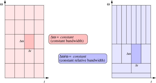
Figure 1: Time-frequency resolution of the windowed Fourier transform (left) vs. time-frequency resolution of the wavelet transform (right), where $\Delta t$ is the time resolution, $\Delta\omega$ is the frequency resolution, and $\Delta t\cdot\Delta\omega=\mathit{constant}\geq\frac{1}{2}$ (Heisenberg uncertainty principle).

1 INTRODUCTION

$N$-body simulations of structure formation in the early Universe, of galaxies and plasmas are limited crucially by noise (e.g., Dawson 1983; Birdsall & Langdon 1991; Pfenniger 1993; Pfenniger & Friedli 1993; Splinter et al. 1998; Baertschiger & Sylos Labini 2002; Hamana, Yoshida & Suto 2002; Huber & Pfenniger 2002; Semelin & Combes 2002). The number of particles $N$ that can be used is several orders of magnitude smaller than the real number of bodies. This implies that fluctuations of physical quantities become drastically exaggerated, and that their contribution to the overall dynamics can even become dominant. One way to reduce noise in simulations is to soften the interaction at short distances. Softening can be optimized so as to suppress small-scale fluctuations while respecting the large-scale dynamical properties (Romeo 1994, 1997, 1998a, b; Dehnen 2001; see also Byrd 1995 and references therein). On the other hand, noise also manifests itself as large-scale fluctuations, and the only known way to reduce them is to increase $N$. This is very uneconomical because the computational cost scales at best linearly with $N$.

Wavelets are a new mathematical tool that has proved to be of great help for noise reduction in digital signal/image processing (see the beautiful presentation by Mackenzie et al. 2001; see also Bergh, Ekstedt & Lindberg 1999). The basic idea behind wavelets is that they provide a multi-resolution view of the signal. The signal is analysed first at the finest resolution consistent with the data, and then at coarser and coarser resolution levels. Doing so, wavelets probe the structure of the signal and the contributions from its various scales. This is fundamental for noise reduction, since noise is present on all scales in the signal. Using wavelets we can thus remove most of the noise without altering the inherent structure of the signal. And we can do this very quickly because the algorithm is even faster than the fast Fourier transform.

So why not use wavelets for reducing noise in simulations? This is indeed the goal of our paper. The idea behind such an application is to de-noise simulations at each timestep. The resulting improvement is of unprecedented level compared with classical techniques: wavelet de-noising makes the simulation equivalent to a simulation with two orders of magnitude more particles.

We provide convincing evidence that our wavelet method works so successfully by making a detailed prediction and carrying out three hard tests. The prediction is based on the improvement in signal-to-noise ratio for initial models of disc galaxies. The tests are devoted to probing the effects of both noise and wavelet de-noising on the simulations, with $N$ spanning two orders of magnitude. Specifically:

1. The first test concerns the fragmentation of a cool galactic disc, which is the onset of a gravitational instability (see, e.g., Binney & Tremaine 1987). We show that the time at which the disc fragments is artificially shortened in simulations with moderate $N$, whereas wavelet de-noising produces an output comparable to simulations with very large $N$, as predicted.

2. The second and third tests concern the heating and accretion following the fragmentation, respectively. These are fundamental processes in the dynamical evolution of disc galaxies, which is induced by gravitational instabilities via the outward transport of angular momentum and energy (see, e.g., Binney & Tremaine 1987). So these tests also have a clear physical motivation. Simulations with moderate $N$ show artificially enhanced heating and accretion, whereas wavelet de-noising produces an output consistent with the prediction.

Even though the prediction and the tests are specific to disc galaxies, our wavelet method is also expected to work successfully when applied to cosmological and plasma simulations. This is because the result depends mainly on the intrinsic properties of wavelets and on the type of noise in the simulation, as we explain incisively in the discussion.

The rest of our paper is organized as follows. The method is presented in Sect. 2, where we give an overview of wavelets and data de-noising using wavelets, and explain how to use them for de-noising $N$-body simulations. The prediction is made in Sect. 3, the three tests are carried out in Sect. 4, and further points are discussed in Sect. 5. Finally, the conclusion is drawn in Sect. 6.

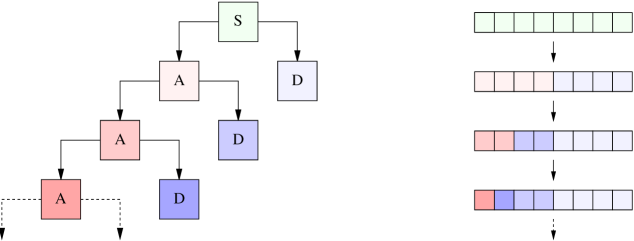
Figure 2: Action of the fast wavelet transform (left) and structure of the transformed signal (right), where ‘S’ is the signal, ‘A’ are the approximations produced by low-pass filtering and down-sampling, and ‘D’ are the details produced by high-pass filtering and down-sampling.

2 METHOD

2.1 Wavelets

Wavelets are a new, very successful, tool for analysing signals, which has exciting applications in physics, apart from engineering and mathematics (see, e.g., Mallat 1998; Bergh et al. 1999). In general, real signals are nonstationary, cover a wide range of frequencies, contain transient components; and the characteristic frequencies of given segments of the signal are correlated with their time durations, in the sense that low/high frequencies imply long/short times. The standard Fourier analysis is inappropriate for such signals because it loses all information about the time localization of a given frequency component, is very uneconomical and highly unstable with respect to perturbations. So real signals require a simultaneous time-frequency analysis.

In general, a linear time-frequency transform can be written as

$$s(t)\mapsto S(a,b)=\int_{-\infty}^{\infty}\psi_{ab}^{\ast}(t)s(t)\mathrm{d}t,$$ (1)

where $s(t)$ is the signal, $S(a,b)$ is the transformed signal at scale $a$ (frequency $\sim 1/a$) and position $b$, and $\psi_{ab}(t)$ is the analysing function. In the windowed Fourier transform,

$$\psi_{ab}(t)=\mathrm{e}^{\mathrm{i}t/a}\psi(t-b),$$ (2)

where the $a$-dependence is a modulation, the $b$-dependence is a translation, and hence the windows $\psi_{ab}(t)$ have the same width as the basic $\psi(t)$. Fig. 1 (left) shows that this transform has a fixed time-frequency resolution. In the wavelet transform,

$$\psi_{ab}(t)=\frac{1}{\sqrt{a}}\psi\left(\frac{t-b}{a}\right),$$ (3)

where the $a$-dependence is a dilation ($a>1$) or a contraction ($a<1$), the $b$-dependence is a translation, and hence the wavelets $\psi_{ab}(t)$ are self-similar to the basic $\psi(t)$. Fig. 1 (right) shows that such a transform has an adaptive time-frequency resolution, which is an important property in favour of its choice. The inverse wavelet transform is

$$S(a,b)\mapsto s(t)=\frac{1}{c_{\psi}}\int_{-\infty}^{\infty}\mathrm{d}b\int_{0}^{\infty}\frac{\mathrm{d}a}{a^{2}}\psi_{ab}(t)S(a,b),$$ (4)

where $c_{\psi}$ is a normalization constant; and, under rather general assumptions, the admissibility condition for its existence is

$$\int_{-\infty}^{\infty}\psi(t)\mathrm{d}t=0,$$ (5)

i.e. wavelets have zero mean. A more general requirement is

$$\int_{-\infty}^{\infty}t^{n}\psi(t)\mathrm{d}t=0\;\;\;(n=0,1,\ldots,N),$$ (6)

i.e. wavelets have a certain number $N+1$ of vanishing moments. This and other requirements for the choice of $\psi(t)$ are discussed in Sect. 2.2. Summarizing in other words, the continuous wavelet transform has the meaning of a local filtering, both in time and in scale, and is non-negligible only when the wavelet matches the signal.

The continuous wavelet transform can be extended to 2-D signals (images) by operating not only a scaling and a translation but also a rotation on the basic wavelet. And it can also be extended to signals defined on more general manifolds via group representation theory.

The wavelet transform can be discretized by setting $a=2^{j}$ and $b=k\cdot 2^{j}$ ($j,k$ integers), but this condition alone does not guarantee that the set of wavelets is an orthogonal basis. Orthogonality is an important property because it means non-redundancy and thus fast algorithms, and besides it is a physically useful requirement (see Sect. 2.2). Orthogonal and bi-orthogonal wavelet bases can be constructed with a mathematical technique known as multi-resolution analysis. The resulting algorithm is the fast wavelet transform and its complexity is $4MN_{\mathrm{d}}$, where $M$ is the size of the wavelet and $N_{\mathrm{d}}=2^{J}$ ($J$ positive integer) is the size of the discrete signal. This algorithm is faster than the fast Fourier transform, whose complexity is $2N_{\mathrm{d}}\log_{2}\!N_{\mathrm{d}}$, and has a data storage of comparable efficiency. Fig. 2 shows how the fast wavelet transform acts on the signal. The signal is decomposed into two parts: an approximation and a detail. The approximation is produced by passing the signal through a low-pass filter and rejecting every other data point. Analogously, the detail is produced by high-pass filtering and down-sampling. The approximation is then itself decomposed into two parts: a coarser approximation and a coarser detail; and the decomposition is iterated. While the wavelet analysis consists of decomposing the signal by filtering and down-sampling, the wavelet synthesis consists of reconstructing the signal by up-sampling and filtering, and the resulting algorithm is the inverse fast wavelet transform.

The fast wavelet transform can be extended to images and $n$-D signals. The discussion basically follows the 1-D case, except that the signal is decomposed into $2^{n}$ parts: 1 approximation and $2^{n}-1$ details, one for each axis and each diagonal; and so on.

2.2 Data de-noising using wavelets

Note that in this section ‘signal’, ‘time’ and ‘frequency’ also mean ‘image’, ‘space’ and ‘wavevector’, or higher-dimensional counterparts, respectively.

2.2.1 Why do wavelets serve to filter noise so effectively?

The adaptive time-frequency resolution and the non-redundancy of the fast wavelet transform have an important practical application: given a noisy signal, the underlying regular part gets mostly concentrated into few large wavelet coefficients, whereas noise is mostly mapped into many small wavelet coefficients. This means that, if we identify a correct threshold, then we can set all the small coefficients to zero and get back a signal almost decontaminated from noise. This is the idea behind data de-noising and explains why wavelets serve to filter noise so effectively, independent of general properties of the data such as the number of dimensions or the presence of symmetries (see, e.g., Mallat 1998; Bergh et al. 1999).

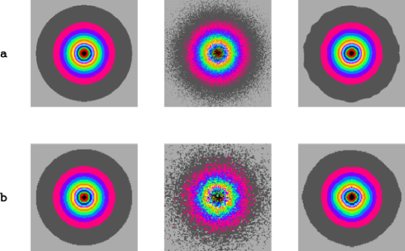
Figure 3: Wavelet de-noising in action. a: set of models with $N=10^{6}$ particles, and with a physical grid of $N_{\mathrm{c}}=512\times 512$ cells and cell size $\Delta_{\mathrm{c}}=0.125$ kpc. The particle distribution is shown for the theoretical model (left), the noisy model (middle) and the wavelet de-noised model (right). In the noisy model the signal-to-noise ratio $\mathit{SNR}\simeq 9.0$, whereas in the wavelet de-noised model $\mathit{SNR}\simeq 85.4$. Thus we predict that wavelet de-noised simulations using this initial model are equivalent to noisy simulations with approximately 90 times more particles, given the Poissonian statistics of noise. b: set of models with $N=10^{5}$, $N_{\mathrm{c}}=256\times 256$ and $\Delta_{\mathrm{c}}=0.25$ kpc, organized as above (from left to right). In the noisy model $\mathit{SNR}\simeq 5.7$, whereas in the wavelet de-noised model $\mathit{SNR}\simeq 37.2$. Thus we predict that wavelet de-noising improves the performance of the relevant simulations by approximately a factor of 42. Such a prediction is tested in Figs 4–6.

2.2.2 Handling two relevant types of noise

In the case of Gaussian white noise, a correct threshold can be identified rigorously if the wavelet basis is orthogonal. The threshold is proportional to the standard deviation of noise, which can be robustly estimated from the smallest-scale detail coefficients, and the proportionality factor depends on the size of the signal.

In the case of Poissonian noise, there is a method that produces good results. The method is to transform the Poissonian data $Y_{\mathrm{P}}$ into data $Y_{\mathrm{G}}$ with (additive) Gaussian white noise of standard deviation $\sigma_{\mathrm{G}}=1$:

$$Y_{\mathrm{G}}=2\,\sqrt{Y_{\mathrm{P}}+{\textstyle\frac{3}{8}}}$$ (7)

(Anscombe 1948), which can then be de-noised as discussed above. Specifically, the Anscombe transformation has the property to help achieving additivity, normalization and variance stabilization (Stuart & Ord 1991). On the other hand, it has a tendency to fail locally where the data have small values or large variations (e.g., Kolaczyk 1997; Starck, Murtagh & Bijaoui 1998). Those features may give rise to negative values in the de-noised data, which can be set to zero. The Anscombe transformation also introduces a bias in the data (e.g., Kolaczyk 1997; Starck et al. 1998). The bias is additive and bounded, can be estimated analytically as

$$\mathit{BIAS}\simeq-\frac{1}{4}\left(1-\frac{1}{N_{\mathrm{d}}}\right)\sigma_{\mathrm{G}}^{2}$$ (8)

(Stuart & Ord 1991) or computed numerically and removed from the de-noised data.

2.2.3 How should we choose the wavelet?

In order to optimize data de-noising, we should choose a wavelet that satisfies the following requirements: (1) it has a small compact support and is symmetric, for a good time localization; (2) it has a large number of vanishing moments and is regular, for a good frequency localization; (3) it is orthogonal, for a correct threshold identification. On the other hand, orthogonal wavelets are not symmetric, with one uninteresting exception. The best alternative is to choose a symmetric bi-orthogonal wavelet that is also quasi-orthogonal. These rules select a few wavelets, from the more than a hundred commonly used. The final choice depends on the resolution required by the data.

2.3 De-noising of $N$-body simulations using wavelets

2.3.1 How does it work?

$N$-body simulations commonly use a grid for tabulating the particle density, and for computing the potential and the field (see, e.g., Hockney & Eastwood 1988). The number of particles $n$ in each cell shows fluctuations $|\delta n|/\langle n\rangle\sim\langle n\rangle^{-1/2}$ with respect to an average $\langle n\rangle$. This means that the particle distribution is corrupted by noise that is basically Poissonian, whereas the noise induced in the potential and in the field is of a more complex nature. Using wavelets we can thus de-noise the particle distribution at each timestep and make the simulation equivalent to a simulation with many more particles. This is how it works.

2.3.2 Which choices of the wavelet are appropriate?

A very appropriate choice for de-noising of $N$-body simulations is the wavelet ‘rbio 6.8’, described in the documentation of the Matlab Wavelet Toolbox (Misiti et al. 1997). This wavelet differs significantly from zero in an interval of approximately three mesh sizes, which is consistent with the effective spatial resolution of the simulations. In simulations dominated by small-scale structures, the wavelet ‘rbio 4.4’ may be a better choice.

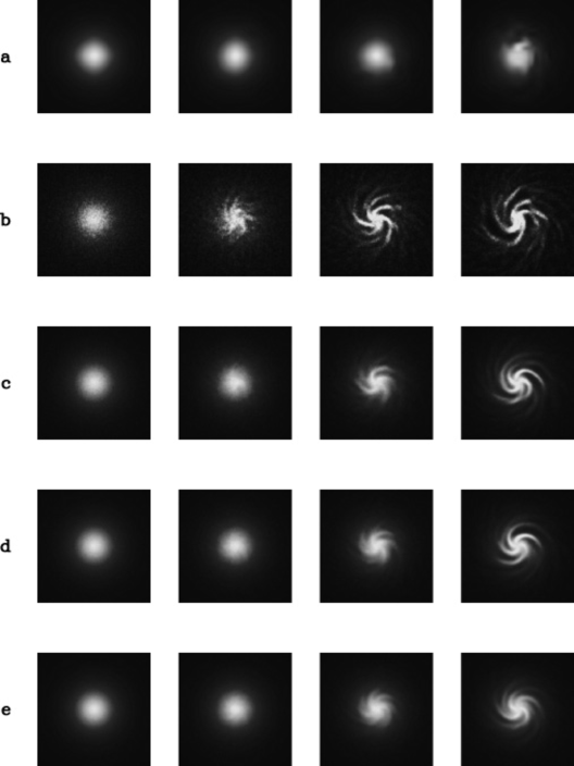
Figure 4: Fragmentation of a cool galactic disc. a: wavelet de-noised simulation with $N=10^{5}$; b: noisy simulation with $N=10^{5}$; c: noisy simulation with $N=1.8\times 10^{6}$; d: noisy simulation with $N=4.2\times 10^{6}$; e: noisy simulation with $N=9\times 10^{6}$. Apart from the number of particles, the initial models are the same as in Fig. 3b. For each simulation, the particle distribution is shown from 0 Myr to 150 Myr at intervals of 50 Myr (from left to right). The time $\tau$ at which the initial axial symmetry breaks is a measure of the effect of noise on the simulation: a long $\tau$ means a weak effect. As expected, $\tau$ increases from b to e. Note that $\tau$ is longer in a than in e. Thus wavelet de-noising improves the performance of the simulation by more than a factor of 90, according to the $\tau$-diagnostic. Such an improvement is well beyond the predictions based on the initial models (cf. Fig. 3b and text).

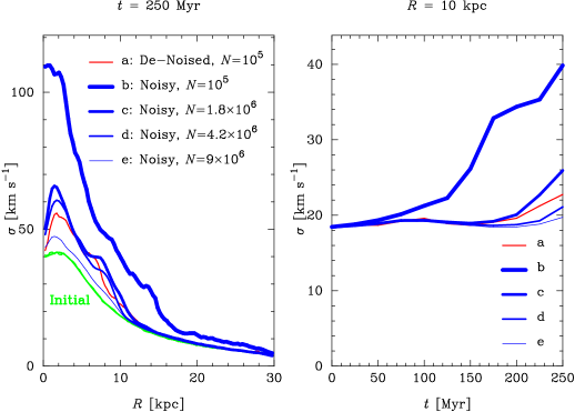
Figure 5: Heating following the fragmentation of a cool galactic disc. The simulations are the same as in Fig. 4. The velocity dispersion $\sigma$ is shown as a function of radius $R$ at the initial and final times, and as a function of time $t$ at an intermediate radius. The increase of velocity dispersion $\Delta\sigma(R)$ from the initial to the final value is a measure of the effect of noise on the simulation: a small $\Delta\sigma$ means a weak effect. In all simulations, except b, heating is significant only for $R\la 10$ kpc. As expected, $\Delta\sigma_{\mathrm{b}}>\cdots>\Delta\sigma_{\mathrm{e}}$. Note that $\Delta\sigma_{\mathrm{a}}<\Delta\sigma_{\mathrm{d}}$ for $R\la 5$ kpc and $\Delta\sigma_{\mathrm{a}}\sim\Delta\sigma_{\mathrm{d}}$ with oscillations for $R\ga 5$ kpc. Thus wavelet de-noising improves the performance of the simulation by a factor of 42 or more, according to the $\Delta\sigma$-diagnostic. This improvement is better than predicted with the initial models (cf. Fig. 3b and text).

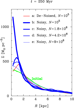
Figure 6: Accretion following the fragmentation of a cool galactic disc. The simulations are the same as in Fig. 4. The mass density $\Sigma$ is shown as a function of radius $R$ at the initial and final times. The peak of final mass density $\hat{\Sigma}$ near the centre gives an estimate of the effect of noise on the simulation: a low $\hat{\Sigma}$ suggests a weak effect. As expected, $\hat{\Sigma}_{\mathrm{b}}>\cdots>\hat{\Sigma}_{\mathrm{e}}$. Note that $\hat{\Sigma}_{\mathrm{a}}<\hat{\Sigma}_{\mathrm{d}}$. Thus wavelet de-noising improves the performance of the simulation by a factor of 42 or more, according to the $\hat{\Sigma}$-diagnostic. This improvement is better than predicted with the initial models (cf. Fig. 3b and text).

3 PREDICTION

In order to make specific predictions, we focus on $N$-body simulations of disc galaxies, and adopt a widely used Cartesian code (Combes et al. 1990). We choose realistic theoretical models that represent a truncated Kuzmin disc of scale length $a_{\mathrm{d}}=5$ kpc and cut-off radius $R_{\mathrm{cut}}=30$ kpc for various $N$, $N_{\mathrm{c}}$ and $\Delta_{\mathrm{c}}$, where $N$ is the number of particles, $N_{\mathrm{c}}$ is the number of cells in the physical grid and $\Delta_{\mathrm{c}}$ is the cell size (see, e.g., Binney & Tremaine 1987). We then create noisy simulation models by generating random particle positions and tabulating $n$ at this initial time. We finally de-noise such models using the wavelet ‘rbio 6.8’. The amount of noise in the models is quantified by the signal-to-noise ratio

$$\mathit{SNR}=\left[\frac{{\displaystyle\sum}\,X_{ij}^{2}}{{\displaystyle\sum}\,(Y_{ij}-X_{ij})^{2}}\right]^{1/2}\,,$$ (9)

where $X_{ij}$ are the theoretical data and $Y_{ij}$ are either the noisy data or the wavelet de-noised data. In the de-noised data, $\mathit{SNR}$ means the inverse of an appropriately defined estimation error.

Fig. 3 illustrates wavelet de-noising in action in a high-resolution case (Fig. 3a) and in a low-resolution case (Fig. 3b). First of all, note that in the noisy simulation models $\mathit{SNR}\propto\sqrt{\bar{n}}$ for a given grid size $\sqrt{N_{\mathrm{c}}}\cdot\Delta_{\mathrm{c}}$, where $\bar{n}=N/N_{\mathrm{c}}$ is the average number of particles per cell. This is consistent with the fact that the noise is basically Poissonian. Then it follows that wavelet de-noising can improve the signal-to-noise ratio by one order of magnitude, as if the noisy model had two orders of magnitude more particles (cf. Fig. 3a). Even in noisy models with low signal-to-noise ratios the improvement is comparable (cf. Fig. 3b). The natural prediction is that the improvement shown for the initial models implies a comparable improvement in performance for the simulations.

4 TESTS

4.1 Fragmentation of a cool galactic disc

In order to test such a prediction, we explore a hard problem: the fragmentation of a cool galactic disc (e.g., Semelin & Combes 2000; Huber & Pfenniger 2001). A rotating disc with low velocity dispersion is gravitationally unstable and therefore sensitive to perturbations, which are amplified and break the initial axial symmetry of the system. The time that characterizes symmetry breaking clearly depends on the initial amplitude of the perturbations, for small perturbations need a long time to grow into an observable level. In particular, this is true for the fluctuations imposed by granular initial conditions. Thus the symmetry-breaking time is a clear diagnostic for quantifying the effect of noise on the simulation. Our initial models are as in Fig. 3b, with the following additional specifications (irrelevant in that context): disc mass $M_{\mathrm{d}}=5\times 10^{10}$ M_⊙, Plummer bulge-halo of comparable mass and scale length, Plummer softening with softening length $s=0.25$ kpc, Safronov-Toomre parameter $Q=0.7$ (see, e.g., Binney & Tremaine 1987). We vary $N$ so as to test in detail the improvements predicted by Fig. 3b, and by an analogous examination of the gravitational field of the disc (a factor of 18). We run the simulations for 250 Myr, a typical dynamical time.

Fig. 4 illustrates that in the wavelet de-noised simulation the symmetry-breaking time is even longer than in the best noisy simulation, which uses the largest number of particles allowed by computer memory. This is a strong piece of evidence that wavelet de-noising outperforms the predictions.

4.2 Heating following the fragmentation of a cool galactic disc

As an additional test, we investigate the heating following the fragmentation of a cool galactic disc. When spiral gravitational instabilities reach a sufficiently large amplitude, the velocity dispersion of the disc starts to increase by collective relaxation (e.g., Zhang 1998; Griv, Gedalin & Yuan 2002). The heat produced in a dynamical time is low if the initial amplitude of the instabilities is small. Therefore the increase of velocity dispersion is another diagnostic for quantifying the effect of noise on the simulation.

Fig. 5 illustrates that, on the whole, in the wavelet de-noised simulation the increase of velocity dispersion is smaller than in the noisy simulation with 42 times more particles. This is a further piece of evidence that wavelet de-noising outperforms the predictions.

4.3 Accretion following the fragmentation of a cool galactic disc

As a further test, we analyse the accretion following the fragmentation of a cool galactic disc. The amplification of spiral gravitational instabilities produces not only heating but also re-distribution of matter in the disc, which appears more evidently as accretion near the centre (e.g., Zhang 1998; Griv et al. 2002). The mass accreted in a dynamical time is low if the initial amplitude of the instabilities is small. So the peak of mass density is still another diagnostic for quantifying the effect of noise on the simulation.

Fig. 6 strengthens our result by confirming, once again, that wavelet de-noising outperforms the predictions.

5 DISCUSSION

Wavelet de-noising suppresses almost all the noise but introduces slight local biases, which have no significant effect on the conservation of angular momentum and energy. In fact, the deviations are less than 0.04% and 0.06% per dynamical time, respectively, and compare well with those typical of the code (Combes et al. 1990). The improvement in performance concerns not only the fidelity of simulations to real systems, shown in Figs 3–6 and discussed above, but also the standard computational issues (time, memory and storage). This improvement is by one/two orders of magnitude in the low/high-resolution case examined. Note in this context that an important, albeit non-classical, reason for increasing the number of particles is to improve the resolution. Optimal choices of $N$, $\Delta_{\mathrm{c}}$ and $s$ are interdependent (e.g., Hernquist, Hut & Makino 1993; Dehnen 2001), and besides they strongly depend on the physical problem under investigation (Romeo 1998a; Dehnen 2001). Wavelet de-noising acts so as to increase the equivalent number of particles, therefore analogous considerations apply. Further points are discussed below.

5.1 Large vs. small spatial scales

The spatial scales on which noise is ‘significant’ depend upon what physical quantity is considered: the particle density, the potential, the field, or other quantities related to the dynamical effect of noise such as the relaxation time (in this case one often refers to the relative contribution of distant and close encounters; e.g., Dehnen 2001). In particular, the particle distribution is affected by noise that is basically Poissonian and white, and hence significant on all scales. As noted in Sect. 2.2 and adapted to the present context, wavelets succeed in suppressing this type of noise not only on small but also on large scales, without damping real instabilities. Indeed, this is what makes wavelets so successful in comparison with other methods of noise reduction (see the literature quoted).

5.2 3D vs. 2D, and initial (a)symmetry

The prediction and the tests shown in previous sections concern disc galaxies, whose simulation models are commonly flat and initially axisymmetric. Appropriate 3-D tests regarding this or other types of galaxies would demand an exceedingly large number of particles, $N\sim 10^{8}\mbox{--}10^{9}$, in order to have a satisfactory signal-to-noise ratio in the basic simulation (an average of a few particles per cell) and in order to be able to run simulations with two orders of magnitude more particles. On the other hand, as noted in Sect. 2.2.1, the remarkable efficiency of wavelets in suppressing noise is an intrinsic property of such functions, which has been tested extensively in the literature. Because of that the initial symmetry is also irrelevant, apart from the fact that it breaks quickly. If any remark should be made, then note that axisymmetry is an unfavourable initial condition since the fast wavelet transform has privileged directions: the Cartesian axes and diagonals (see Sect. 2.1). Thus the result of our paper is also expected to hold in 3D, with or without initial symmetry.

5.3 Plasma and cosmological vs. galaxy simulations

Can our wavelet method be applied to plasma and cosmological simulations?

The case of plasma simulations is rather clear. Even if the initial models are non-noisy, Poissonian noise develops in few dynamical times (see, e.g., Dawson 1983; Birdsall & Langdon 1991). Wavelet de-noising can be applied from the start, since it prevents the onset of noise without affecting the quiet model.

The case of cosmological simulations is more complex but is also quite clear. The initial conditions consist of setting up a non-noisy uniform particle distribution, and of imposing small random fluctuations with Gaussian statistics and a given power spectrum (e.g., Efstathiou et al. 1985; Sylos Labini et al. 2002). Poissonian noise develops naturally, as a reaction of the system to the initial order and hence reduced entropy. The onset of Poissonian noise is especially quick in cold-dark-matter simulations, where structures form bottom-up and the first virialized systems contain a small number of particles (e.g., Binney & Knebe 2002). There is a natural way to apply our wavelet method to cold-dark-matter simulations. It is to de-noise them only over a range of scales that is adapted to the phase of clustering: from the cell size to the size of the structures that have formed latest. Analogous ideas can be implemented in the context of other cosmological models. In this way wavelet de-noising prevents the onset of Poissonian noise without affecting the imposed fluctuations, or the quiet background.

Thus our wavelet method can be applied not only to galaxy but also to cosmological and plasma simulations, with minor adaptions.

6 CONCLUSION

The conclusion of this paper is that wavelet de-noising allows us to improve the performance of $N$-body simulations up to two orders of magnitude. This result has been shown for simulations of disc galaxies, and can be generalized to other grid geometries and particle species than those used here. Besides, wavelet de-noising can be adapted for a variety of constraints (e.g., partial de-noising at given scales or at a pre-assigned level) and initial conditions (e.g., partially noisy or quiet starts), and thus have important applications also in cosmological and plasma simulations.

Our wavelet code will be described in a following paper, and will then be available on request.

References

- [1] Anscombe F. J., 1948, Biometrika, 35, 246
- [2] Baertschiger T., Sylos Labini F., 2002, Europhys. Lett., 57, 322
- [3] Bergh J., Ekstedt F., Lindberg M., 1999, Wavelets. Studentlitteratur, Lund
- [4] Binney J., Knebe A., 2002, MNRAS, 333, 378
- [5] Binney J., Tremaine S., 1987, Galactic Dynamics. Princeton University Press, Princeton (errata in astro-ph/9304010)
- [6] Birdsall C. K., Langdon A. B., 1991, Plasma Physics via Computer Simulation. Institute of Physics Publishing, Bristol
- [7] Byrd G., 1995, in Hunter J. H. Jr., Wilson R. E., eds, Ann. N. Y. Acad. Sci. 773, Waves in Astrophysics. N. Y. Acad. Sci., N. Y., p. 302
- [8] Combes F., Debbasch F., Friedli D., Pfenniger D., 1990, A&A, 233, 82
- [9] Dawson J. M., 1983, Rev. Mod. Phys., 55, 403
- [10] Dehnen W., 2001, MNRAS, 324, 273
- [11] Efstathiou G., Davis M., Frenk C. S., White S. D. M., 1985, ApJS, 57, 241
- [12] Griv E., Gedalin M., Yuan C., 2002, A&A, 383, 338
- [13] Hamana T., Yoshida N., Suto Y., 2002, ApJ, 568, 455
- [14] Hernquist L., Hut P., Makino J., 1993, ApJ, 402, L85 (erratum in ApJ, 411, L53)
- [15] Hockney R. W., Eastwood J. W., 1988, Computer Simulation Using Particles. Institute of Physics Publishing, Bristol
- [16] Huber D., Pfenniger D., 2001, A&A, 374, 465
- [17] Huber D., Pfenniger D., 2002, A&A, 386, 359
- [18] Kolaczyk E. D., 1997, ApJ, 483, 340
-
[19]
Mackenzie D. et al., 2001,
in Beyond Discovery: The Path from Research to Human Benefit –
Wavelets: Seeing the Forest and the Trees. National Academy of
Sciences, Washington (
http://www.BeyondDiscovery.org/) - [20] Mallat S., 1998, A Wavelet Tour of Signal Processing. Academic Press, San Diego
- [21] Misiti M., Misiti Y., Oppenheim G., Poggi J.-M., 1997, Wavelet Toolbox for Use with Matlab: User’s Guide. The MathWorks, Natick
- [22] Pfenniger D., 1993, in Combes F., Athanassoula E., eds, -Body Problems and Gravitational Dynamics. Observatoire de Paris, Paris, p. 1
- [23] Pfenniger D., Friedli D., 1993, A&A, 270, 561
- [24] Romeo A. B., 1994, A&A, 286, 799
- [25] Romeo A. B., 1997, A&A, 324, 523
- [26] Romeo A. B., 1998a, A&A, 335, 922
- [27] Romeo A. B., 1998b, in Salucci P., ed., Dark Matter. Studio Editoriale Fiorentino, Firenze, p. 177
- [28] Semelin B., Combes F., 2000, A&A, 360, 1096
- [29] Semelin B., Combes F., 2002, A&A, 388, 826
- [30] Splinter R. J., Melott A. L., Shandarin S. F., Suto Y., 1998, ApJ, 497, 38
- [31] Starck J.-L., Murtagh F., Bijaoui A., 1998, Image Processing and Data Analysis: The Multiscale Approach. Cambridge University Press, Cambridge
- [32] Stuart A., Ord J. K., 1991, Kendall’s Advanced Theory of Statistics – Vol. 2: Classical Inference and Relationship. Hodder & Stoughton – Arnold, London
- [33] Sylos Labini F., Baertschiger T., Gabrielli A., Joyce M., 2002, in press (astro-ph/0211058)
- [34] Zhang X., 1998, ApJ, 499, 93