Multi-Color Light Curves of Type Ia Supernovae on the Color-Magnitude Diagram: a Novel Step Toward More Precise Distance and Extinction Estimates

Abstract

We show empirically that fits to the color-magnitude relation of Type Ia supernovae after optical maximum can provide accurate relative extragalactic distances. We report the discovery of an empirical color relation for Type Ia light curves: During much of the first month past maximum, the magnitudes of Type Ia supernovae defined at a given value of color index have a very small magnitude dispersion; moreover, during this period the relation between $B$ magnitude and $B-V$ color (or $B-R$ or $B-I$ color) is strikingly linear, to the accuracy of existing well-measured data. These linear relations can provide robust distance estimates, in particular, by using the magnitudes when the supernova reaches a given color. After correction for light curve strech factor or decline rate, the dispersion of the magnitudes taken at the intercept of the linear color-magnitude relation are found to be around 0^m.08 for the sub-sample of supernovae with $(B_{max}-V_{max})$ $\leq\ 0^{m}.05$, and around 0^m.11 for the sub-sample with $(B_{max}-V_{max})$ $\leq\ 0^{m}.2$. This small dispersion is consistent with being mostly due to observational errors. The method presented here and the conventional light curve fitting methods can be combined to further improve statistical dispersions of distance estimates. It can be combined with the magnitude at maximum to deduce dust extinction. The slopes of the color-magnitude relation may also be used to identify intrinsically different SN Ia systems. The method provides a tool that is fundamental to using SN Ia to estimate cosmological parameters such as the Hubble constant and the mass and dark energy content of the universe.

1 Introduction

SNe Ia provide reliable measurements of extragalactic distances. The conventional method depends on accurate observations near optical maxima and detailed light curve shapes to deduce luminosity corrections from the initial decline rates or the time scale stretch factor of the light curves (Pskovskii, 1977; Phillips, 1993; Perlmutter et al., 1997), or luminosity corrections from lightcurve shape fits (Riess et al., 1996). Existing observations and theories indicate that SN Ia are indeed excellent distance indicators in spite of concerns about several systematic effects such as gray dust, evolution and asymmetry. Relative magnitudes accurate to about $15\%$ have been deduced based on supernovae observed in the redshift range from about 3000 km/sec to 30,000 km/sec (Hamuy et al., 1994; Riess et al., 1996; Phillips et al., 1999). It has also been shown that a two parameter luminosity correction which employs fits to $\Delta m_{15}$ and $(B_{max}-V_{max})$ can further reduce the magnitude dispersion (Tripp, 1997; Tripp & Branch, 1999).

All of the existing light curve analysis methods aim at deriving magnitudes at maximum light and the parameters governing the shapes of the observed light curves. The method by Hamuy et al. (1993); Phillips (1993) employs a number of well observed supernova light curves to model observed light curves to derive simultaneously the magnitude at maximum and the light curve decline rate $\Delta m_{15}$ (the $B$ magnitude decline from the peak at 15 days after explosion). Another approach called the multi-color light curve shape method (MLCS) was introduced by Riess et al. (1996, 1999) which makes joint fits to light curves at different colors to obtain simultaneously the magnitudes at different colors, the light curve shape corrections to the magnitudes, and the color-excesses (Riess et al., 1996). This approach attempts, within a certain class of models, to statistically determine the best indicator of luminosity. Alternatively, Perlmutter et al. (1997) introduced a time-scale stretch parameter to quantify the shapes of SN light curves. It was found that stretch describes the observed $B$ and $V$ band light curves well over a month around maximum (Goldhaber et al., 2001). Attempts to derive other parameters from the morphology of Type Ia light curves that are correlated with the magnitude at optical maximum are reported in Hamuy et al. (1996a, b).

While the magnitude at maximum has been used as a standard value, there is no physical reason as to why this magnitude is superior to the magnitude at other epochs. As shown by the various published analyses, the maximum magnitudes can be corrected by a one or two parameter relation to reduce the scatter in absolute magnitude to less than 15%. If SNe Ia are indeed a one or two parameter family, it is in principle possible to deduce distance measurements from any points on the light curve, provided that required parameters for correcting the measured magnitudes can be found, by methods such as light curve shapes or spectroscopy (e.g. Nugent et al. 1995; Riess et al. 1998).

In this paper, we outline a Color-Magnitude Intercept Calibration (CMAGIC) method that concentrates on multi-color post-maximum light curves of SNe Ia and makes use of their color information. We discovered an empirical color relation for Type Ia light curves: During much of the first month past maximum, the magnitudes of Type Ia supernovae defined at a given value of color index have a very small magnitude dispersion; moreover, during this period the relation between $B$ magnitude and $B-V$ color (or $B-R$ or $B-I$ color) is strikingly linear, to the accuracy of existing well-measured data. We will employ the extinctions given by Phillips et al. (1999) for most of this study, but we will also show that our method can provide reliable independent estimates of extinction. We show that accurate calibration can be obtained without data around optical maximum. This method suggests new observational strategies to obtain accurate distance estimates. The complete analysis presented in this paper was made for $B$-magnitude vs $B-V$ Color. We will also discuss $B-R$ and $B-I$ colors, but will present a more thorough study in a later paper. We emphasize that this is a new method for calibrating SN Ia as distance measurements and more work is in progress.

2 The Method

We analyze the data of the nearby supernova samples published by Hamuy et al. (1996a), Riess et al. (1999), and Krisciunas et al. (2001). For each supernova we study the relationship between $B$ and $B-V$ (the “Color-Magnitude” or “CMAG” plot) as shown in the bottom panels of Figures 1-4 for a few example supernovae. The complete set of CMAG plots of well-measured supernovae are shown in Appendix A. Figures A1, A2, and A3 are for $B$ versus $B-V$, $B$ versus $B-R$, and $B$ versus $B-I$, respectively.

The immediate post-maximum CMAG evolution of all these supernovae except SN 1992K show a period during which the observed $B$ magnitude and the various colors are linearly related. The examples shown in Figures 1-4 exhibit some variations in behavior outside this linear region. In general, it is convenient to write the color-magnitude relations as

$$B\ =\ B_{BV}\ +\ \beta_{BV}\ (B-V)$$

$$B\ =\ B_{BR}\ +\ \beta_{BR}\ (B-R)$$

$$B\ =\ B_{BI}\ +\ \beta_{BI}\ (B-I)$$

Here $\beta_{BV}$, $\beta_{BR}$, and $\beta_{BI}$ give the slopes of the curves, and for linear $B$ versus $B$-$V$, $B$-$R$, and $B$-$I$ relations, $B_{BV}$, $B_{BR}$, and $B_{BI}$ are constants in time for each fit to an individual supernova. The slopes $\beta$ are defined equivalently by

$$\beta_{BV}\ =\ \dot{B}/(\dot{B}-\dot{V})$$

$$\beta_{BR}\ =\ \dot{B}/(\dot{B}-\dot{R})$$

$$\beta_{BI}\ =\ \dot{B}/(\dot{B}-\dot{I})$$

Note that equations (2) are valid not only in the linear regime of the CMAG relation but can also be used to describe the non-linear parts of the CMAG curves, although this study is dedicated only to the linear regime of the CMAG relation. As we will see in the following sections, the supernovae behave very uniformly in the linear region, but less so in the before and after regions, therefore we will focus only on the linear region in this study.

The linear regime can be explored for its uniformity and applications to distance determination. Direct extrapolation of the linear fits to $(B-V)$ = 0, $(B-R)$ = 0, and $(B-I)$ = 0 would give values for intercepts $B_{BV}$, $B_{BR}$, and $B_{BI}$. However, these values would introduce extrapolation errors correlated with the errors in $\beta_{BV}$, $\beta_{BR}$, and $\beta_{BI}$. In practice, such correlated errors can be minimized by calculating a magnitude close to the mean of the various colors. In this study, we focus only on $B$ and $V$ band data. As we shall see, the mean color $<B-V>$ is typically around 0${}^{m}.6$ and the $K$-corrected $<$$\beta_{BV}$$>$ is typically 1.94. For consistency across different studies, it is convenient to define an arbitrary reference color that is close to the color average for each pair of bands. The intercept of $B-V$ = 0^m.6 and the line describing the linear region (as given in equations (1a) and (2a)) defines a magnitude $B_{BV0.6}$ that is least correlated to the errors of fitting slope. For convenience in comparing to $B_{max}$, we will use $B_{BV}\ \equiv\ B_{BV0.6}\ -\ 1.94\times 0^{m}.6\ =\ \ B_{BV0.6}\ -\ 1^{m}.164$ throughout this paper as the standard color magnitude intercept.

The fitted values of $B_{BV}$ and $\beta_{BV}$ are shown in Table 1 for all of these supernovae for which more than 3 data points on the post maximum linear region of the CMAG plot are available. A two day gap is introduced around the Transition-Date (cf §2.1 and captions to Figure 1) where the data points are not included in the linear fits. Various SNe exhibit different color behavior during the epoch before and after the linear region but nearly all show very similar behavior during the linear region with small variations in the value of the slope.

Table 1: Fits to Post-Maximum Light Curves of SN Ia

SN	$log_{(}cz)$	B${}_{BV}(\sigma)$	B${}^{fix}_{BV}(\sigma)$	$\beta_{BV}(\sigma)$	Bmax	$(B_{max}-V_{max})$	$\Delta m_{15}$($\sigma$)	${E_{BV}}(B-V)$($\sigma$)	Hubble Type
(1)	(2)	(3)	(4)	(5)	(6)	(7)	(8)	(9)	(10)
1990O	3.957	16.53 (014 )	16.52 (047 )	2.07 (02 )	16.59 (08 )	0.01	0.96 (10 )	0.15 (03 )	SBa
1990T	4.080	17.22 (010 )	17.21 (008 )	1.88 (01 )	17.27 (20 )	0.04	1.15 (10 )	0.08 (04 )	SA(s)00
1990Y	4.070	16.95 (137 )	17.00 (028 )	2.05 (12 )	17.69 (20 )	0.33	1.13 (10 )	0.13 (06 )	E(M32?)
1990af	4.178	17.74 (037 )	17.71 (021 )	2.10 (08 )	17.91 (03 )	0.05	1.56 (05 )	0.08 (02 )	SB0
1991S	4.222	17.85 (084 )	17.87 (031 )	1.72 (15 )	17.78 (20 )	0.04	1.04 (10 )	0.04 (05 )	Sb
1991U	3.968	16.53 (047 )	16.53 (020 )	1.90 (05 )	16.67 (20 )	0.06	1.06 (10 )	0.10 (04 )	Sbc:pec
1991ag	3.617	14.76 (071 )	14.77 (014 )	1.96 (07 )	14.67 (13 )	0.08	0.87 (10 )	0.09 (04 )	SB(s)dmPec
1992J	4.137	17.44 (159 )	17.51 (019 )	2.08 (14 )	17.88 (20 )	0.12	1.56 (10 )	0.10 (04 )	S
1992ae	4.351	18.54 (051 )	18.52 (038 )	2.08 (08 )	18.64 (10 )	0.11	1.28 (10 )	0.09 (03 )	E1?
1992ag	3.890	16.23 (114 )	16.21 (068 )	1.80 (13 )	16.64 (05 )	0.13	1.19 (10 )	0.21 (05 )	S?
1992al	3.626	14.80 (013 )	14.72 (020 )	2.18 (04 )	14.59 (03 )	-0.05	1.11 (05 )	0.03 (01 )	SAB(s)c
1992aq	4.481	19.10 (063 )	19.16 (033 )	1.60 (14 )	19.39 (07 )	0.10	1.46 (10 )	0.12 (04 )	Sa?
1992au	4.261	18.13 (255 )	18.09 (046 )	1.71 (32 )	18.17 (20 )	0.05	1.49 (10 )	0.02 (06 )	E1
1992bc	3.773	15.61 (038 )	15.62 (017 )	1.93 (05 )	15.15 (03 )	-0.08	0.87 (05 )	0.02 (01 )	Sab
1992bg	4.029	17.19 (031 )	17.18 (026 )	2.11 (05 )	17.39 (05 )	-0.04	1.15 (10 )	0.20 (03 )	Sa
1992bh	4.131	17.47 (037 )	17.49 (030 )	2.05 (04 )	17.68 (05 )	0.08	1.05 (10 )	0.18 (03 )	Sbc
1992bk	4.240	18.06 (030 )	18.07 (044 )	1.64 (05 )	18.07 (08 )	0.00	1.57 (10 )	0.01 (04 )	S0-pec
1992bl	4.110	17.36 (055 )	17.34 (036 )	2.05 (09 )	17.34 (05 )	0.00	1.51 (10 )	0.01 (03 )	(R1)SB(s)0/a
1992bo	3.735	15.78 (036 )	15.78 (009 )	1.99 (06 )	15.85 (03 )	0.01	1.69 (05 )	0.03 (01 )	SB(s)00pec
1992bp	4.374	18.41 (057 )	18.46 (045 )	1.72 (11 )	18.53 (03 )	-0.05	1.32 (10 )	0.11 (03 )	E2/S0
1992br	4.420	19.14 (055 )	19.17 (076 )	1.64 (08 )	19.34 (16 )	0.04	1.69 (10 )	0.05 (05 )	E0
1992bs	4.279	18.33 (047 )	18.32 (030 )	2.02 (08 )	18.33 (06 )	0.07	1.13 (10 )	0.08 (03 )	Sc(s)II
1993B	4.326	18.36 (055 )	18.43 (033 )	1.61 (12 )	18.81 (09 )	0.12	1.04 (10 )	0.24 (05 )	SBb
1993H	3.862	16.30 (051 )	16.31 (021 )	2.00 (06 )	16.99 (05 )	0.23	1.69 (10 )	0.24 (04 )	SB(r)ab
1993O	4.192	17.76 (055 )	17.76 (023 )	2.08 (07 )	17.79 (03 )	-0.09	1.22 (05 )	0.09 (02 )	E5/S01
1993ac	4.169	18.14 (029 )	18.17 (026 )	2.18 (03 )	18.45 (15 )	0.20	1.19 (10 )	0.20 (04 )	E
1993ae	3.734	15.50 (115 )	15.54 (037 )	2.10 (13 )	15.40 (20 )	-0.07	1.43 (10 )	0.04 (05 )	E
1993ag	4.176	17.82 (046 )	17.82 (025 )	2.01 (06 )	18.30 (07 )	0.03	1.32 (10 )	0.24 (04 )	E3/S01
1993ah	3.947	16.52 (072 )	16.50 (063 )	1.65 (09 )	16.32 (20 )	-0.04	1.30 (10 )	0.02 (05 )	E
1994M	3.860	16.32 (074 )	16.27 (039 )	2.10 (22 )	16.35 (05 )	0.05	1.44 (10 )	0.04 (03 )	E
1994Q	3.939	16.39 (056 )	16.39 (019 )	1.95 (10 )	16.40 (19 )	-0.04	1.03 (10 )	0.06 (04 )	S0
1994S	3.686	15.06 (028 )	15.06 (013 )	1.97 (03 )	14.79 (07 )	-0.04	1.10 (10 )	0.02 (02 )	Sbc
1994ae	3.208	13.31 (040 )	13.31 (012 )	1.96 (06 )	13.21 (07 )	0.11	0.86 (05 )	0.10 (03 )	Sc
1995D	3.293	13.59 (023 )	13.53 (024 )	2.33 (05 )	13.44 (07 )	0.02	0.99 (05 )	0.08 (02 )	S0
1995E	3.540	15.33 (081 )	15.33 (020 )	1.95 (07 )	16.82 (07 )	0.73	1.06 (05 )	0.52 (04 )	Sb
1995ac	4.166	17.21 (027 )	17.19 (016 )	2.07 (05 )	17.19 (07 )	0.08	0.91 (05 )	0.13 (03 )	S
1995ak	3.824	16.05 (068 )	16.04 (025 )	1.90 (07 )	16.28 (10 )	0.10	1.26 (10 )	0.12 (04 )	Sbc
1995al	3.188	13.25 (124 )	13.23 (053 )	1.78 (15 )	13.36 (07 )	0.12	0.83 (05 )	0.12 (05 )	SA(rs)bc:
1995bd	3.681	15.99 (130 )	16.10 (027 )	2.14 (10 )	17.27 (10 )	0.79	0.84 (05 )	0.62 (07 )	S
1996C	3.955	16.66 (019 )	16.65 (018 )	1.83 (02 )	16.59 (10 )	0.07	0.97 (10 )	0.07 (04 )	Sa
1996X	3.308	13.17 (026 )	13.19 (033 )	2.15 (03 )	13.26 (07 )	0.05	1.25 (05 )	0.11 (02 )	E0
1996Z	3.357	13.84 (053 )	13.84 (031 )	2.46 (08 )	14.61 (10 )	0.36	1.22 (10 )	0.28 (04 )	Sb
1996bl	4.019	16.89 (033 )	16.88 (018 )	1.87 (03 )	17.08 (07 )	0.15	1.17 (10 )	0.17 (03 )	SBc
1996bo	3.714	15.32 (068 )	15.33 (021 )	1.99 (07 )	16.15 (10 )	0.41	1.25 (05 )	0.31 (04 )	Sc
1996bv	3.700	15.26 (053 )	15.26 (027 )	2.01 (08 )	15.77 (13 )	0.25	0.93 (10 )	0.26 (05 )	Scd:
1999dk	3.618	14.79 (092 )	14.78 (034 )	1.92 (14 )	15.06 (10 )	0.15	1.00 (10 )	0.16 (05 )	???
2000bk	3.902	16.55 (031 )	16.56 (011 )	1.99 (03 )	16.98 (20 )	0.17	1.63 (10 )	0.08 (04 )	???
2000ce	3.695	16.12 (141 )	16.16 (040 )	2.01 (11 )	17.24 (20 )	0.61	0.99 (10 )	0.22 (06 )	???

Note. — The columns are: (1) name of the supernova; (2) redshift; (3) the Color-Magnitude with errors in units of 0^m.001; (4) the Color-Magnitude for fixed slope fit with errors in units of 0^m.001; (5) the fitted slope with error in units of 0.01; (6) the magnitude at maximum as reported in Hamuy et al. (1996a); Riess et al. (1996); Krisciunas et al. (2001), with errors in 0^m.01; (7) the color at maximum; (8) $\Delta m_{15}$ as reported in Hamuy et al. (1996a); Riess et al. (1996); Krisciunas et al. (2001); (9) the host galaxy extinction derived from CMAGIC after applying the Bayesian prior as described in Phillips et al. (1999); (10) host galaxy type

Both colors and magnitudes are subject to observational errors. The errors on $B$-$V$ colors are not available for most of the supernovae; when unavailable they are constructed from the published errors of $B$ and $V$ by assuming uncorrelated errors and are calculated by the square root of the sum of the square of the errors on $B$ and $V$ for each SN. This is normally an overestimate of the errors in most cases, and the errors thus constructed are correlated to those at individual colors. These errors were taken into account in the linear fits and indeed, in most cases the resulting $\chi^{2}$ per degree of freedom values were less than one. Since it is hard to track the exact nature of the correlations of the errors we therefore scaled the color and magnitude errors to make $\chi^{2}_{\nu}\ =\ 1$. We note that this does not change the fitting parameters significantly, but only the final errors associated with them. Alternatively, one can also fit linear relations between $B$ and $V$ directly and then convert the fitted parameters to $B_{BV}$. We found no significant differences between the two approaches and will use the $B$ vs $B-V$ fits for clarity.

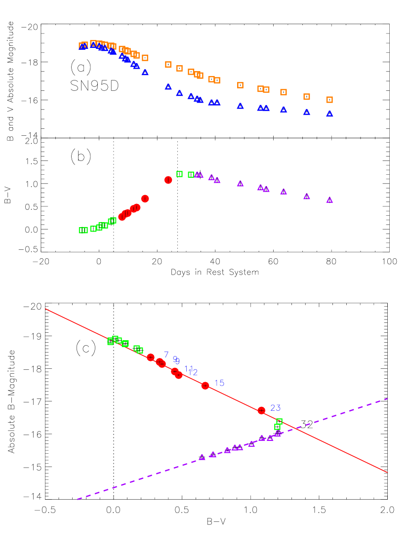
Figure 1: Example of a SNe that is typical of the majority of SNe in our sample. (a) The lightcurve in the B-band (blue triangles) and V-band (orange squares).(b) Color vs. Rest-frame day plot. The two vertical lines bracket the linear epoch. The green squares and purple triangles show data outside the linear region. The linear region is shown in red circles. (c) The Color-Magnitude plot. The epoch before and soon after the linear region is shown in green open squares. The epoch of the linear region is shown in red filled circles. The epoch after the linear region which corresponds to the nebular phase is shown in violet open triangles. For the linear region the rest frame days after $B$ maximum are given by the blue numbers. The red line is the CMAGIC fit to the linear region with slope $\beta_{BV}$. The violet dashed line is the fit to the nebular phase region. The intersection of these two lines is marked with the day (in black) of the abrupt change in color evolution.

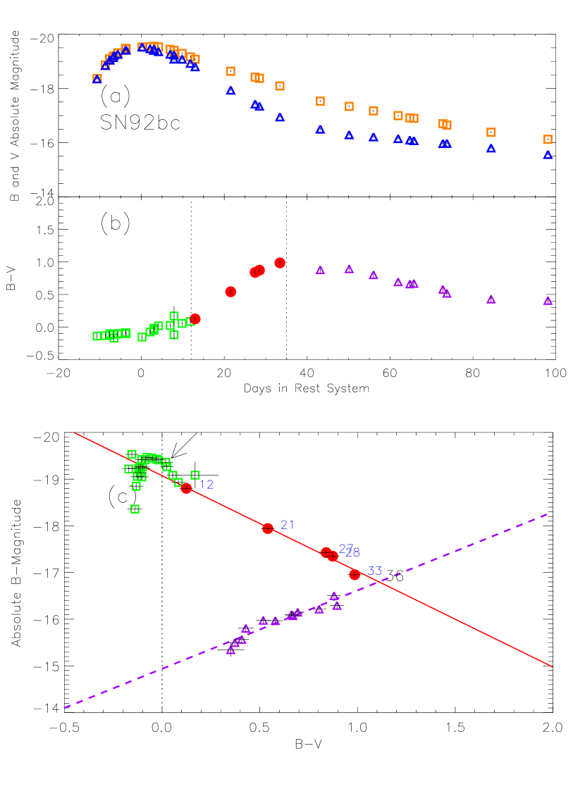
Figure 2: Example of a SNe that exhibits the “bump” feature (cf. §2.1). The bump is marked by the arrow in the figure. This SN which is very bright and has high stretch, low $\Delta m_{15}$ and low extinction. See caption to Figure 1.

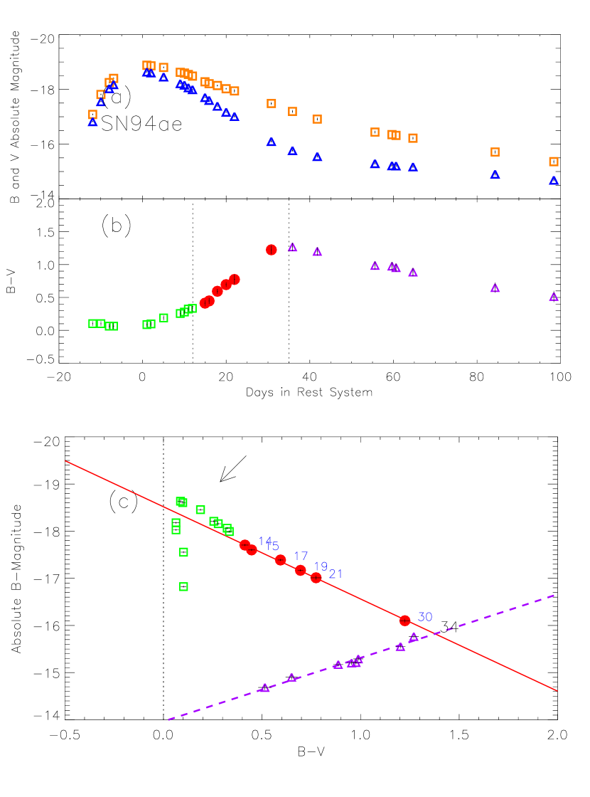
Figure 3: Example of another SNe that exhibits the “bump” feature. The bump is marked by the arrow in the figure. This SN has also a low $\Delta m_{15}$, with large dust extinction however. See caption to Figure 1.

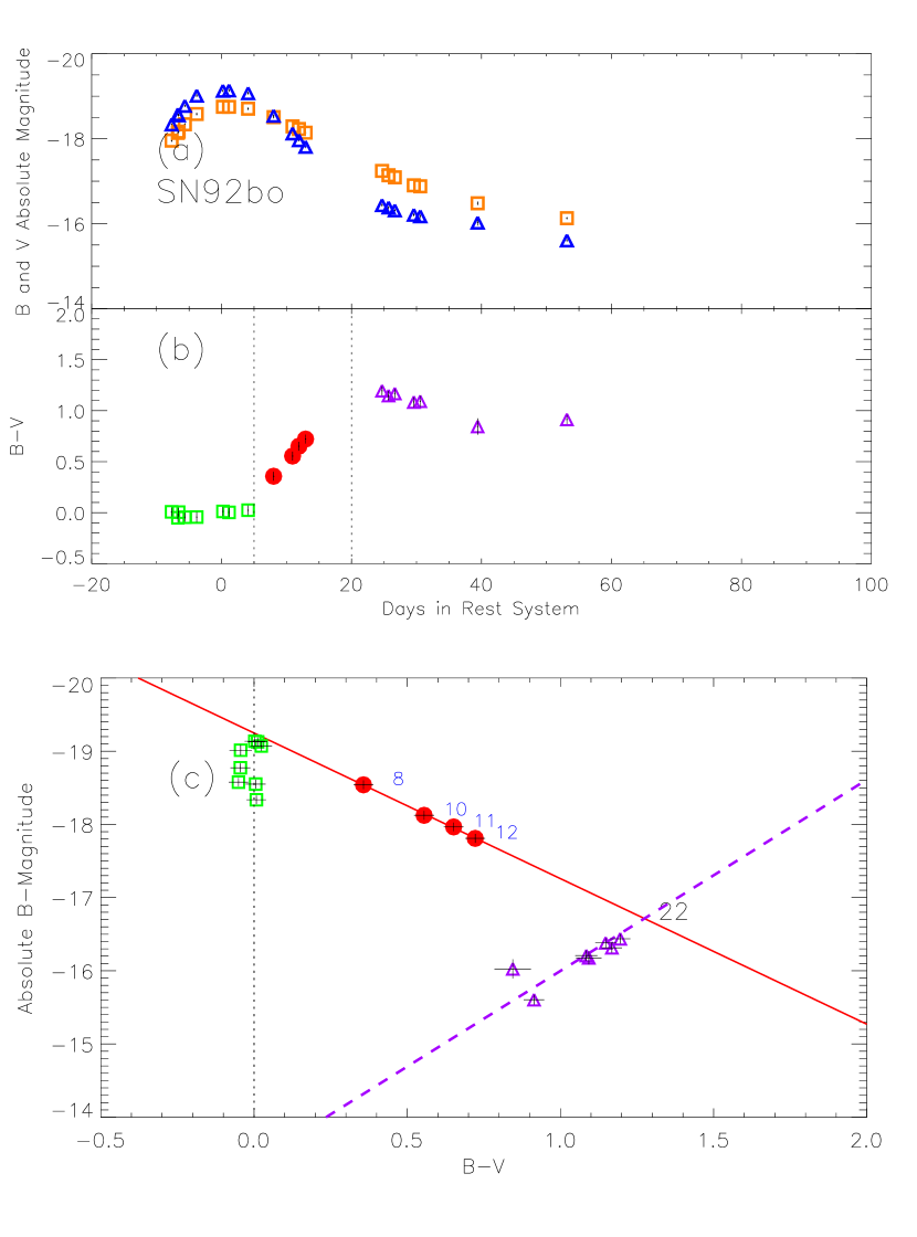
Figure 4: A second example of a SN that does not exhibit the “bump” feature. This SN is very dim with large $\Delta m_{15}$. The Transition-Date is earlier than for supernovae with smaller $\Delta m_{15}$. See caption to Figure 1.

SN 1992K is the only supernova in this sample which does not show a linear relation with $\beta_{BV}$ around 2. In fact, the $B-V$ and $B-I$ colors never exhibited a redward evolution during the course of the observations. It is an intrinsically dim SN Ia with a very fast light curve ($\Delta m_{15}\ =\ 1^{m}.93$) and spectral evolution that is very similar to that of SN 1991bg (Hamuy et al., 1994). This supernova was discovered after optical maximum. It is likely that the linear regime was either not observed, or does not exist for this particular peculiar supernova. For this reason, SN 1992K is excluded from further consideration. Such peculiar supernovae are easy to identify and can be excluded by the shape of the color-magnitude curve.

2.1 The Shapes of the Color-Magnitude Diagrams of Type Ia Supernovae

In Figures 1 to 4 we show a number of well measured SNe as examples to illustrate the CMAGIC method for the $B$-band with $B$-$V$ color. All data points shown in Figures 1 to 4 have been K-corrected to the rest system. In these Figures (a) we first plot the $B$ and $V$ lightcurves in absolute magnitudes (assuming $H_{0}$ = 65 km/sec/kpc). The color, for each set of data points, is then the difference between the two curves. In (b) we show the color vs the epoch in the SN rest frame. In (c) we show the absolute $B$-magnitude vs the color $B-V$. The linear regime is identified on the CMAG plot (c) and is marked by red points. As we will discuss, the epoch over which the linear region occurs varies in its starting and ending day, and these dates are correlated with the stretch factor or the rate of magnitude decline $\Delta m_{15}$. We have shown the early data before and around maximum light in green, the linear region in red and the tail or nebular phase region in violet. We have indicated the day for each data point for the linear region in blue. We have fitted the linear region (red data points) to obtain the slope $\beta_{BV}$. We have also fitted the nebular phase region shown in violet in Figures 1 to 4, which is also linear in this representation. The intersection of these two lines is marked with the day (in black) at which the color evolution changes abruptly from $B-V$ increasing linearly towards the red to decreasing linearly. For comparison, Lira (1995); Riess et al. (1996); Phillips et al. (1999) noticed a different linear relation between $B$ magnitude versus time during the nebular phase. Further analysis of supernovae well observed both around optical maxima and up to the nebular phase shows that $\Delta m_{15}$ are strongly correlated with the date the supernovae reaches maximum (reddest) $B-V$ values. This correlation can be seen in plots given in Phillips et al. (1999) and Garnavich et al. (2001). Details of this will be presented in another separate paper.

As shown in Figures 1-4, and A1, the evolution of a typical Type Ia supernova normally starts at $B-V$ around 0 or bluer before optical maximum, and it evolves rapidly to the red soon after optical maximum. In the tail region or during the “supernebular” phase the CMAG plot takes a sharp turn and then evolves rapidly towards the blue. This sharp turn defines another characteristic time – the Transition-Date at which the supernova reaches the nebular phase. This date corresponds approximately to the ”inflection point” on the light curves of SN Ia discussed in Pskovskii (1977), Pskovskii (1984), and Pavlyuk et al. (1998), or the ”intersection point” in Hamuy et al. (1996b). The morphology of the evolutionary track is determined by the derivatives given in equations (2). The shapes of the CMAG relations are therefore insensitive to extinction, redshift, and the stretch values of the light curves if $s_{B}\ \propto\ s_{V}$, where $s_{B}$ and $s_{V}$ are the stretch parameters in the $B$ and $V$ bands, respectively. Extinction only displaces the entire CMAG curve but does not change its shape. Redshift stretches the time coordinates, by $1+z$, equally in all colors and does not change the slopes given in equation (2). The shapes of the color-magnitude plots are dependent, but only indirectly, on redshift and extinction via K-correction. These properties as well as the simple linearity with very small dispersions make CMAG a powerful tool for studying intrinsic properties of supernovae.

We derive from Figures 1-4, and A1-3 the CMAGIC linear relation of Type Ia supernovae: linear relations between $B$ magnitude and $B-V$, $B-R$, and $B-I$ colors, universal to SN Ia during much of the first month past maximum exist for Type Ia supernovae.

The variations in CMAG curves outside the linear region indicate that Type Ia light curves are not a one parameter family. In a one parameter family, a supernova is characterized by a single variable such as the stretch factor, or $\Delta m_{15}$. In previous studies, it was found that the stretch factor of different colors are correlated. When the extended Leibundgut (1988) templates are used, a relation $s_{V}\ =\ s_{B}$ (Perlmutter et al., 1997, 1999; Goldhaber et al., 2001) was found to approximately describe the Type Ia light curves for matching $B$ and $V$ templates. Real scatter on the $s_{B}$ versus $s_{V}$ diagram was indeed observed but was difficult to distinguish from observational errors. The CMAG diagram provides a new way to investigate this issue. If a fixed linear relation exists for stretch at different colors and the light curve at each color is universal to all the supernovae with $s_{B}$ the only free parameter, to first order, we would expect the CMAG curves and $\beta_{BV}$ as defined in equations (2) to be universal as well. This would imply that regardless of the light curve shapes, all the Type Ia supernovae should show identical morphology on the CMAG diagram.

The CMAG diagrams shown in Figures 1 to 4 and Figures A1, A2, and A3 appear not to agree with the single parameter model outside the linear region. On these $B$ versus $(B-V)$ graphs, the $B$ magnitudes increase rapidly while the colors show relatively small evolution until the supernova reaches $B$ maximum. After that, the supernovae can be divided into at least two groups. The first group shows a “bump” of excess luminosity (typically before day 12) above the linear fits at around the maximum, and the other does not.

Examples of the SN Ia showing a bump are: SN 1992bc, SN 1994ae, SN 1995al, SN 1995bd, SN 1996C, and SN 1996ab. Members of this group are among the brightest Type Ia supernovae. Spectroscopic data identified 1995bd as a SN 1991T-like event (Garnavich et al., 1995). The $\Delta m_{15}$ values for these supernovae are around 0.87 – the lowest end of the templates used to determine these parameters (Phillips et al., 1999; Hamuy et al., 1996b; Riess et al., 1996). For this group of supernovae, the epochs at which the linear regimes apply are typically from 12 to 35, 11 to 33, and 11 to 32 days after optical maximum in the $B$ versus $B-V$, $B$ versus $B-R$, and $B$ versus $B-I$ diagrams, respectively. SN 1991ag and SN 1992P are the only two supernovae, in the sample studied, with $\Delta m_{15}$  about 0.87 for which the $B$ versus $(B-V)$ graphs do not show obvious bumps. This seems to be due mostly to the incomplete observation time coverages. For SN 1991ag, a hint of a bump can in fact be seen when a linear CMAG fit is applied to data between day 12 to 35. No color information is available between day 12 to 35 for SN 1992P. This group of supernovae includes also SN 1991T, SN 1997br (Li et al., 1999), and SN 2000cx (Li et al., 2001), not in our sample but well observed. However, it should be noted that the spectroscopically SN 1991T-like event - SN 1995ac (Filippenko & Leonard, 1995) does not show the bump that defines this group.

Most of the supernovae fall into the second group for which the CMAG diagrams are linear and without a bump. Typical epochs of the linear region ranges from day 5 to 27, 11 to 31, and 11 to 32 for $B$ versus $(B-V)$, $B$ versus $(B-R)$, and $B$ versus $(B-I)$, respectively. But some supernovae such as SN 1992bk, SN 1992bo, and SN 1993ae show a considerably shorter duration of the linear region which lasts only about 16 days from day 5 to 20 for $B$ versus $B-V$. These are typically intrinsically dimmer supernovae with values of $\Delta m_{15}$ above 1.4. We note that the peculiar SN 1991bg and SN 1999by (Garnavich et al., 2001) show linear regions on CMAG plot similar to the one shown in Figure 4. Other supernovae with comparable $\Delta m_{15}$  for which however not enough late epoch data are available to constrain their evolution around day 27, are SN 1992aq, SN 1992au, SN 1992br, SN 1993H, SN 1994M, and SN 1996bk. Their behavior on the CMAG diagram are similar.

In Figure 5 we show the composite residuals of the linear fits rebinned to $B-V$ intervals of 0.1. The value at each interval is given by the weighted average of all the residuals of the linear fits within that bin. Errors on both $B$ and $B-V$ were taken into account in these calculations. No systematic deviations from a straight line are observed down to the 0${}^{m}.01$ level to which this data is sensitive. For most of the very well observed supernovae, the fits usually give $\chi^{2}$ per degree of freedom well below 1, and typical scatter around the fits is less than 0^m.05. This demonstrates that on average linear fits indeed provide an accurate description of the observed data. At least for the currently available data, higher order fits, or more complicated color-magnitude templates are not necessary.

Figure 5: Mean composite residuals of the linear fits to the $B$ versus $B-V$ curves, binned to $B-V$ interval of 0.1. The small residual values indicate that the data can be very well described by a straight line.

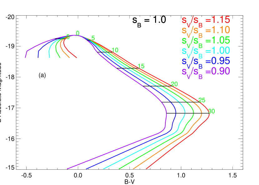
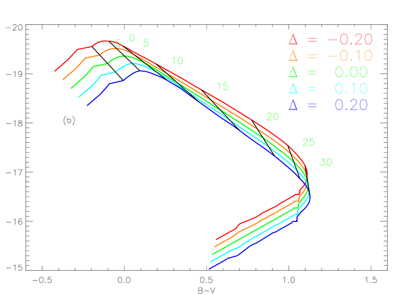
Figure 6: (a) Absolute Magnitude versus Color plot from $B$ and $V$ standard templates each stretched by $s_{B}$ and $s_{V}$ respectively. The small numbers correspond to the epoch of the light curve in days from $B$ maximum. In this illustrative example $s_{B}$ = 1.0 is kept fixed while $s_{V}$ varies from 0.90 to 1.15. Reading from left to right at day 15, the curves correpond to different stretch ratios from $s_{V}/s_{B}$ = 0.90 to 1.15. Note that the linear relations are qualitatively reproduced, and that both the light curves without a bump and with a bump are qualitatively reproduced from differences of stretched standard templates (Leibundgut, 1988; Perlmutter et al., 1997, 1999; Goldhaber et al., 2001). (b) The color curves obtained from the templates of Riess et al. (1996) with varying correction coefficients $\Delta$. Reading from bottom to top at day 15, the different curves correpond to $\Delta$ values from 0^m.2 to -0^m.2 as shown in the figure. The linear relations are well reproduced, but the templates fail to reproduce any supernovae with a bump.

A possible elaboration of the stretch fitting model to account for the the behavior on the CMAG Diagram outside the linear region can be constructed by assuming a series of different ratios of the $B$ and $V$ stretches $s_{B}/s_{V}$. This concept is shown in Figure 6 (a), where curves are given for a number of stretch ratios $s_{B}/s_{V}\ =\ 0.90\ -\ 1.15$. The template light curves are the $B$-template ’Parab20’ discussed in Goldhaber et al. (2001), the $V$-templates were treated in a similar fashion. Indeed, the morphology classes of the CMAG Diagram are qualitatively reproduced. Those with a bump typically have $B$ stretch larger than $V$ stretch values, whereas those without a bump have $B$ stretch values smaller or comparable to the $V$ stretch values. It seems that stretch values measured with lightcurves of different colors have the potential of measuring more subtle differences of the light curve properties. However, it should be noted that Figure 6 (a) does not provide quantitative fits to the observed morphology shown in Figures 1 to 4, and A1. The epochs of the linear regimes are inconsistent with the observed values.

For comparison, we plot in Figure 6 (b) the template spectra constructed by Riess et al. (1996) with varying correction coefficients, $\Delta$. The linear relation is successfully reproduced, but the templates fail to reproduce the bumps normally associated with the brightest supernovae. For these supernovae, this may lead to systematic errors in the color estimates near maximum which in turn lead to errors on extinction estimates.

$K$-correction (Oke & Sandage, 1968; Hamuy et al., 1993; Kim et al., 1996; Nugent & et al., 2002) affects the color magnitudes, and were applied to the observed magnitudes before the linear color-magnitude fits. We do not expect significant K-correction errors as the redshifts of the SN Ia are low ($z$ $\lesssim$ 0.1). The linearity of $B$ versus $B-V$, $B-R$, and $B-I$ relations implies that the $K$-correction would likely conserve the linearity of the linear section of the CMAG relation. At these redshifts, an approximate linear relation between the $K$-corrections and the observed colors can be constructed. Therefore for the CMAGIC method, $K$-corrections may be applied either before or after the linear fits to the observed data points. In this study, we have made the $K$-corrections after the linear CMAG fits of the observed data points.

2.2 The Characteristics of the Slope $\beta$

It is found from the relatively well calibrated sample that the mean slopes without $K$-corrections are: $<$$\beta_{BV}$$>\ =\ 2.07\pm 0.18$, $<$$\beta_{BR}$$>\ =\ 1.26\pm 0.10$, $<$$\beta_{BI}$$>\ =\ 0.88\pm 0.09$, where the errors are standard deviations from mean. Typical measurement errors for $\beta_{BV}$ are 0.2, and the measured $\beta$ values are quite consistent for all SN Ia. The small dispersions of the slopes are not a surprise and only confirm that Type Ia supernovae indeed form a relatively uniform class of objects.

Although to first order the slopes $\beta$ are extinction independent, they are weak functions of $K$-corrections which then implies that without applying $K$-corrections, $\beta$ will be a function of supernova redshift. The $K$-corrected fits of the $B$ versus $B-V$ color curves show slopes that are consistently smaller than those without $K$-correction. The $K$-corrected mean slope is $\beta_{BV}$ = $1.94\pm 0.16$.

Histograms of the distribution of the slope $\beta_{BV}$ are shown in Figure 7. To explore the potential of $\beta_{BV}$ as an indicator of intrinsic properties of SN Ia, we have plotted the $\beta_{BV}$ distribution in spirals and that in E+S0 galaxies separately. We have also constructed ideograms of the data by weighing each data point with associated errors (solid lines on Figure 7), and the expected distribution assuming a unique slope of 1.94 weighted by the fitted slope errors of each supernova (dotted lines on Figure 7). For the supernovae in spiral galaxies, the unique slope seems to provide an approximate description of the data. It is interesting to note, however, that the current data set is suggestive of an intrinsic difference between the slope distribution for supernovae in E+S0 galaxies and that in spirals. In particular, a hint of a secondary spike at $\beta_{BV}$ around 1.65 is found for SN Ia from E+S0 but not for those from spirals. Five out of 19 SN Ia with E+S0 hosts have $\beta_{BV}$ around 1.65, whereas only two of 28 in spirals were found to have $\beta_{BV}$ $\leq$ 1.65. The significance of these differences is hard to quantify considering the fact that the data collection process may not be entirely homogeneous. For example, most of the SNe showing slopes around 1.65 were observed around 1992 (cf. Figure 9) which may be indicative of observational biases in the reported magnitudes. A Kolmogorov-Smirnov test gives a probability of 19% for the two distributions to be identical. This is not sufficient to firmly establish a statistical conclusion. Future observations should be able to resolve these issues.

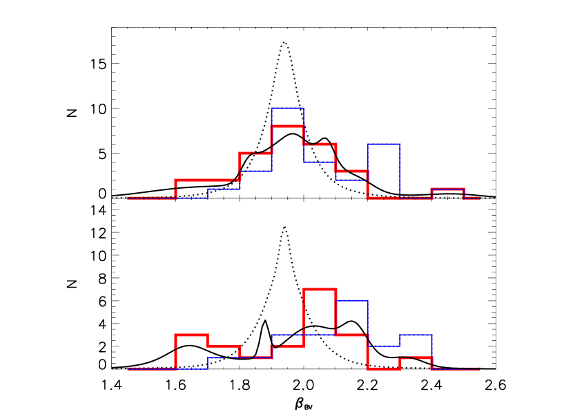
Figure 7: Histograms of the distributions of the slopes of the linear fits. The thin blue lines are without $K$-correction, and thick red lines are with $K$-correction. The smooth solid lines are the ideogram constructed by weighting each data point with associated errors. The dotted line shows the distribution assuming a unique slope of 1.94 and then weighted by the errors of each individual slope. The upper panel is for supernovae in spirals and the lower for supernovae in E+S0 galaxies. More data would help to determine if the distribution in E+S0 galaxies are different from that in spirals.

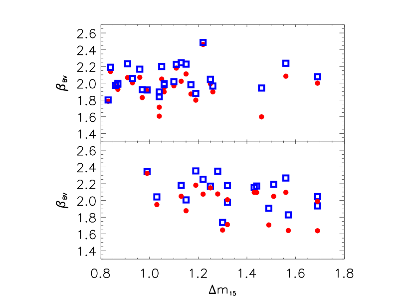
Figure 8: The slopes of the Color-Magnitude fits versus the light curve decline rate $\Delta m_{15}$ for supernovae from spiral(upper panel) and E+S0 (lower panel) hosts. Red circles are for the slopes after $K$-corrections, and blue squares are the data without $K$-corrections. No correlation is seen between the slopes and $\Delta m_{15}$, as is expected from the definitions in equation 2.

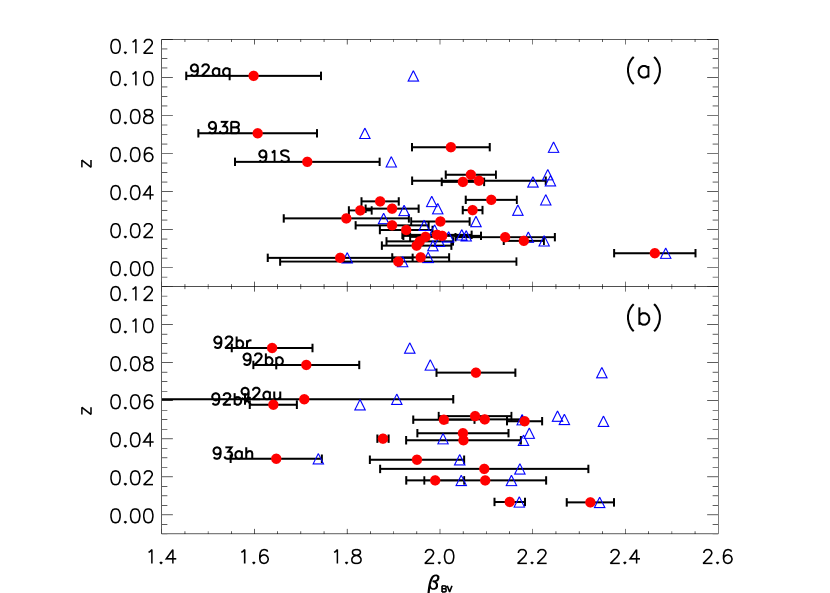
Figure 9: Redshift versus slopes with (filled red circles ) and without (blue triangles) K-corrections for supernovae from spiral (a) and E+S0 (b) galaxies. The secondary enhancement at $\beta_{BV}$ = 1.65 shown in Figure 7(b) is also apparent in (b). The data are suggestive of different branches of supernovae with intrinsically different slopes, but more data are needed to test such differences.

It is interesting to note that $K$-correction does not appreciably decrease the $\beta_{BV}$ dispersion. This might be an indication that we are indeed close to the limits of observational or $K$-correction errors. $K$-corrections are applied under the assumption that the supernovae under study are drawn from samples identical to those used to construct the $K$-corrections. If the assumption is correct, a reduction of slope dispersions is expected. In practice, the $K$-correction was constructed from a sample that is different in the mean from the larger sample we are studying, in a way such that some Type Ia with $\beta_{BV}$ $\sim 1.65$ may be under-represented. A large number of spectroscopically well-observed supernovae are required to construct well calibrated, $K$-corrected slope distributions for different filters. Such distributions can be used for self-consistency checks of evolutionary effect of more distant supernovae. It may even be necessary to employ separate $K$-corrections for SNe with different $\beta_{BV}$ values. Better $K$-corrections can be constructed in the future from systematic spectrophotometric supernova programs such as the Nearby Supernova Factory (Aldering et al., 2002a, b).

As we have already shown from discussions of equations (1) and (2), the slopes $\beta$ are uncorrelated or only weakly correlated to the decline rates or the stretch factors of the supernova light curves. This is easily understood from their definitions in equations (2) where a stretch of both the $B$ and $V$ light curves does not affect the values of the slopes. The slopes change only when the ratios of the $B$ and $V$ stretches varies. And, indeed, as is shown in Figure 8, no obvious correlations of $\beta_{BV}$ can be established with $\Delta m_{15}$, or the stretch factor.

As shown in the previous section and in Figure 6, the slopes of the linear fits are also functions of $K$-correction. For supernovae with stretch factor as the only characteristic parameter, applying $K$-corrections should remove the redshift dependence of $\beta_{BV}$. Figure 9 (a) and 9 (b) show $\beta_{BV}$ and redshift correlation for SNe of spiral and of E+S0 hosts, respectively. The data suggest strongly that the assumption of a single parameter family is not appropriate in describing the variations of $\beta_{BV}$ values. The possible $\beta_{BV}$ enhancement around 1.65 revealed in Figure 7 (b) is seen again in Figure 9 primarily for E+S0 hosts in Figure 9 (b). Comparing Figure 9 (a), and 9 (b) reveals that the incidence of SN Ia in E+S0 shows a possible deficit at $\beta_{BV}$ around 1.85 compared to those in spirals. Note also that SNe below $z\ <\ 0.04$ are more tightly clustered than those at higher redshifts; this is perhaps an indication of $K$-correction errors at higher redshifts.

2.3 The Characteristics of $B_{BV}$

$B_{BV}$  $B_{BR}$, and $B_{BI}$ by definition are characteristic magnitudes of the linear CMAG fits evaluated at certain values of $B-V$, $B-R$, and $B-I$, respectively. These magnitudes can be used to derive distances to the supernovae just as the magnitude at optical maximum, which has been used historically.

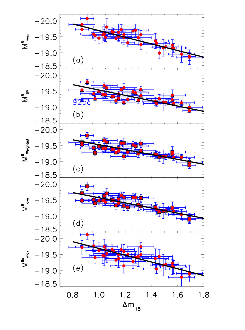
Figure 10: Fits to the magnitudes and $\Delta m_{15}$ relations for $B_{max}$ (a), $B_{BV}$ (b), weighted average of the $B_{max}$ and $B_{BV}$ (c), unweighted average of $B_{max}$ and $B_{BV}$ (d), and $B_{max}$ (e) corrected with extinctions derived from CMAGIC. $R_{B}\ =\ 4.1$ in all fits and the constraint $(B_{max}-V_{max})$ $<$ 0.2 is set to select the data points. In (b) SN 1992bc is rejected from the fits at 3 $\sigma$ level. The solid lines show results from linear fits to the magnitude-$\Delta m_{15}$ relations. The average and weighted average magnitude show moderate improvement over both the original maximum magnitudes and the CMAGs. The magnitude dispersions after the $\Delta m_{15}$ fits are shown in Table 2.

The most remarkable property of these color magnitudes is that extinction corrections to these magnitudes are not given by the conventional $A_{B}\ =\ R_{B}\cdot E(B-V)$. Instead, because of the color dependency of the magnitudes, extinction corrections are given by

$$A_{BV}\ =\ (R_{B}-\beta_{BV})\cdot E(B-V),$$

$$A_{BR}\ =\ R_{B}\cdot E(B-V)\ -\ \beta_{BR}\cdot E(B-R),$$

and

$$A_{BI}\ =\ R_{B}\cdot E(B-V)\ -\ \beta_{BI}\cdot E(B-I),$$

respectively.

With typical values of $R_{B}\ =\ 4.1$, $R_{V}\ =\ 3.1$, $R_{R}\ =\ 2.33$, and $R_{I}\ =\ 1.48$ and an extinction curve that is typical of the Galaxy (Cardelli et al., 1989), we then find

$$A_{BV}\ =(R_{B}\ -\beta_{BV})\cdot E(B-V),$$

$$A_{BR}\ =(R_{B}\ -\ 0.586R_{V}\beta_{BR})\cdot E(B-V),$$

and

$$A_{BI}\ =(R_{B}\ -\ 0.858R_{V}\beta_{BI})\cdot E(B-V),$$

¿From Table 1 where we found $\beta_{BV}$ $\approx$  2, we see that the extinction correction for $B_{BV}$ is typically reduced by nearly 50% of the extinction corrections needed for the original observed magnitudes. The CMAGs are therefore significantly less sensitive to errors in E(B-V) estimates. This is important because in the stretch or $\Delta m_{15}$ corrected magnitudes, errors in $E(B-V)$ are multiplied by about $R_{B}\ \approx\ 4.1$ and could easily become the dominate errors for distance measurements. A 50% reduction of this error is a significant improvement.

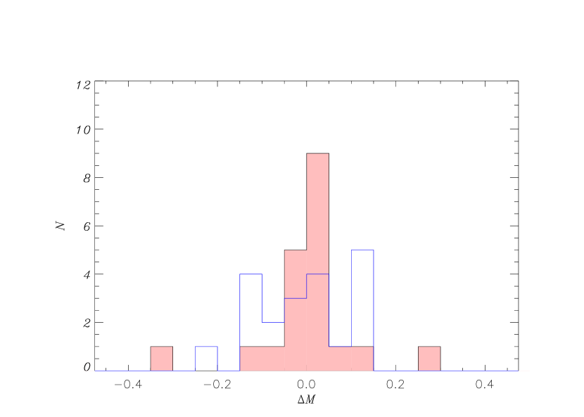
Figure 11: Histograms showing the distribution of the residuals after removing the $\Delta m_{15}$ dependence for a sample of low extinction supernovae with $(B_{max}-V_{max})$ $<\ 0^{m}.05$. Interstellar extinction by the host galaxy is removed assuming $R_{B}\ =\ 3.3$ which gives minimal magnitude dispersion. Apart from two apparent outliers (SN 1992bc and SN 1992bp), the Color-Magnitudes (pink shadowed line) show significantly smaller dispersion than that of the maximum magnitudes (blue solid line). Such improvement becomes less obvious for a larger sample with more highly extincted supernovae included (cf lowest section of Tables 2 and 3), but this tight dispersion may be hard to see given extinction correction uncertainties.

In the analyses that follow, we will only study the supernovae with redshift $z\ >\ 0.01$. To plot the various magnitudes on the Hubble diagram, we assume a peculiar velocity for all the SNe of 250 km/sec, and apply an extinction correction based on the $E(B-V)$ derived by Phillips et al. (1999).

With no $\Delta m_{15}$ or stretch correction, the mean and standard deviations of the absolute color magnitude $M^{B}_{BV}$ for the sample of supernovae with $(B_{max}-V_{max})$ $<\ 0^{m}.05$ are found to be -19^m.26 and 0^m.16, respectively. The corresponding numbers for $M^{B}_{max}$, the absolute magnitude at maximum are -19^m.38 and 0^m.26. This shows that for poorly observed data set where it is impossible to derive reliable $\Delta m_{15}$, the color magnitudes can provide better distance estimates than the magnitudes at maximum.

The magnitude derived above, just like the magnitude at maximum, shows correlations with the light curve decline rate. Figures 10 (a) and 10 (b) show linear fits of the conventional maximum magnitudes and $M^{B}_{BV}$ versus $\Delta m_{15}$, respectively. The fits were performed for supernovae with redshift above 0.01 and $(B_{max}-V_{max})$ $\leq$ 0.2 mag which excluded supernovae with large dust extinction. The color-magnitudes are correlated with $\Delta m_{15}$, as can be seen in Figure 10 (b), but the corrections for $\Delta m_{15}$ dependence are smaller as the slope of the $\Delta m_{15}$ dependence is less steep than that for the maximum magnitudes. Note that SN 1992bc, an SN with a bump on the CMAG plot, deviates more than 3 $\sigma$ from the fitted line for $B_{BV}$. This could be the combination of a few factors such as intrinsic differences of the supernovae and errors in extinction estimates.

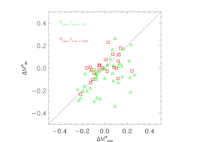
Figure 12: Residuals of the magnitude-$\Delta m_{15}$ relation fits for $M^{B}_{max}$ and $M^{B}_{BV}$ plotted against each other. The red squares are for the subsample of supernovae with the most restrictive color cut $(B_{max}-V_{max})$ $\leq\ 0^{m}.05$, and the green triangles subsample includes less restrictive color cut $(B_{max}-V_{max})$ $\leq\ 0^{m}.05$. Note that the supernovae that are common to both samples appear at different locations on this plot since the $\Delta m_{15}$ relations are different for the two samples. Significant differences between the two magnitudes (i. e., points far from the 45 degree line) are observed only for those with large extinctions.

Table 2: Fit Parameters for $\Delta m_{15}$ Corrections with $R_{B}\ =\ 4.1$

	No Outlier Rejections						Rejecting 3-$\sigma$ Outliers
$M^{B}$	a	$\sigma$a	b	$\sigma$b	$\sigma$	N	a	$\sigma$a	b	$\sigma$b	$\sigma$	N
(1)	(2)	(3)	(4)	(5)	(6)	(7)	(8)	(9)	(10)	(11)	(12)	(13)
Bmax-V${}_{max}\ \leq\ 0.05$ (most restrictive)
max	-19.57	0.04	0.95	0.15	0.10	20	-19.57	0.04	0.95	0.15	0.10	20
BV	-19.33	0.02	0.46	0.08	0.12	20	-19.37	0.03	0.60	0.10	0.10	19
Weighted	-19.40	0.03	0.62	0.10	0.08	20	-19.40	0.03	0.62	0.10	0.08	20
Ave	-19.44	0.03	0.68	0.11	0.09	20	-19.44	0.03	0.68	0.11	0.09	20
EF	-19.09	0.03	-0.07	0.11	0.16	20	-19.09	0.03	-0.07	0.11	0.16	20
${max}^{c}$	-19.58	0.04	1.01	0.12	0.12	20	-19.58	0.04	1.01	0.12	0.12	20
Bmax-V${}_{max}\ \leq\ 0.2$
max	-19.59	0.03	1.04	0.13	0.14	36	-19.59	0.03	1.04	0.13	0.14	36
BV	-19.41	0.02	0.69	0.08	0.16	36	-19.45	0.02	0.83	0.10	0.14	35
Weighted	-19.45	0.02	0.76	0.09	0.13	36	-19.45	0.02	0.76	0.09	0.13	36
Ave	-19.49	0.03	0.80	0.10	0.13	36	-19.49	0.03	0.80	0.10	0.13	36
EF	-19.17	0.02	0.14	0.11	0.21	36	-19.17	0.02	0.14	0.11	0.21	36
${max}^{c}$	-19.58	0.03	1.06	0.12	0.14	36	-19.58	0.03	1.06	0.12	0.14	36
Bmax-V${}_{max}\ \leq\ 0.5$
max	-19.61	0.03	1.12	0.13	0.16	40	-19.61	0.03	1.12	0.13	0.16	40
BV	-19.46	0.02	0.84	0.09	0.22	40	-19.48	0.02	0.89	0.09	0.16	38
Weighted	-19.49	0.02	0.88	0.10	0.18	40	-19.47	0.02	0.84	0.09	0.14	39
Ave	-19.53	0.03	0.89	0.10	0.15	40	-19.51	0.03	0.87	0.10	0.13	39
EF	-19.18	0.02	0.04	0.12	0.24	40	-19.18	0.02	0.04	0.12	0.24	40
${max}^{c}$	-19.58	0.03	1.02	0.11	0.15	40	-19.58	0.03	1.02	0.11	0.15	40

Note. — Fit results to the magnitude – $\Delta m_{15}$ relations for $R_{B}\ =\ 4.1$ expressed in terms of ${\bf M^{B}}\ =\ (a\pm\sigma{a})+(b\pm\sigma b)\cdot\Delta m_{15}$, where $M^{B}$represents one of $M^{B}_{max}$, $M^{B}_{BV}$, $M^{B}_{Weighted}$, $M^{B}_{Ave}$, $M^{B}_{EF}$, or $M^{Bc}_{max}$. Columns 6 and 12 give the weighted deviations from the linear fits, and colums 7 and 13 give the number of supernovae used in the fits.

Table 3: Fit Parameters for $\Delta m_{15}$ Corrections with $R_{B}\ =\ 3.3$

	No Outlier Rejections						Rejeting 3-$\sigma$ Outliers
MB	a	$\sigma$a	b	$\sigma$b	$\sigma$	N	a	$\sigma$a	b	$\sigma$b	$\sigma$	N
(1)	(2)	(3)	(4)	(5)	(6)	(7)	(8)	(9)	(10)	(11)	(12)	(13)
Bmax-V${}_{max}\ \leq\ 0.05$ (most restrictive)
max	-19.55	0.04	0.98	0.13	0.10	20	-19.55	0.04	0.98	0.13	0.10	20
BV	-19.32	0.02	0.50	0.07	0.11	20	-19.35	0.02	0.60	0.08	0.07	18
Weighted	-19.39	0.02	0.63	0.09	0.08	20	-19.39	0.02	0.63	0.09	0.08	20
Ave	-19.43	0.03	0.70	0.10	0.09	20	-19.43	0.03	0.70	0.10	0.09	20
EF	-19.13	0.02	0.14	0.09	0.13	20	-19.13	0.02	0.14	0.09	0.13	20
${max}^{c}$	-19.57	0.03	1.03	0.11	0.11	20	-19.57	0.03	1.03	0.11	0.11	20
Bmax-V${}_{max}\ \leq\ 0.2$
max	-19.55	0.03	1.03	0.12	0.14	36	-19.55	0.03	1.03	0.12	0.14	36
BV	-19.38	0.02	0.77	0.07	0.16	36	-19.38	0.02	0.72	0.08	0.11	32
Weighted	-19.42	0.02	0.81	0.08	0.13	36	-19.43	0.02	0.80	0.08	0.12	35
Ave	-19.45	0.02	0.80	0.09	0.12	36	-19.45	0.02	0.80	0.09	0.12	36
EF	-19.18	0.02	0.30	0.09	0.17	36	-19.18	0.02	0.30	0.09	0.17	36
${max}^{c}$	-19.56	0.03	1.06	0.11	0.14	36	-19.56	0.03	1.06	0.11	0.14	36
Bmax-V${}_{max}\ \leq\ 0.5$
max	-19.56	0.03	1.10	0.11	0.14	40	-19.56	0.03	1.10	0.11	0.14	40
BV	-19.42	0.02	0.84	0.08	0.19	40	-19.44	0.02	0.87	0.08	0.14	37
Weighted	-19.44	0.02	0.86	0.08	0.15	40	-19.43	0.02	0.83	0.07	0.12	38
Ave	-19.47	0.02	0.85	0.09	0.13	40	-19.46	0.02	0.84	0.09	0.12	39
EF	-19.20	0.02	0.26	0.09	0.19	40	-19.20	0.02	0.26	0.09	0.19	40
${max}^{c}$	-19.55	0.03	1.03	0.10	0.14	40	-19.55	0.03	1.03	0.10	0.14	40

Note. — Fit results to the magnitude – $\Delta m_{15}$ relations for $R_{B}\ =\ 3.3$ expressed in terms of ${\bf M^{B}}\ =\ (a\pm\sigma{a})+(b\pm\sigma b)\cdot\Delta m_{15}$, where $M^{B}$ represents one of $M^{B}_{max}$, $M^{B}_{BV}$, $M^{B}_{Weighted}$, $M^{B}_{Ave}$, $M^{B}_{EF}$, or $M^{Bc}_{max}$. Columns 6 and 12 give the weighted deviations from the linear fits, and collums 7 and 13 give the number of supernovae used in the fits.

We have also performed similar fits for different values of $R_{B}$ and color cuts. The resulting fitting parameters are shown in Tables 2 and 3 where we also show the results after rejecting data which deviate by more than 3 sigma from the linear fits. The fits of Tables 2, 3, and 4 were all performed on sub-samples with different cuts on color $(B_{max}-V_{max})$ $<\ 0^{m}.05$, $0^{m}.2$, and $0^{m}.5$. $(B_{max}-V_{max})$ is basically an extinction indicator but is also correlated with intrinsic brightness of a supernova. Although not a requirement of CMAGIC, this cut simultaneously rejects heavily reddened and intrinsically red supernovae above the given threshold. Most entries in Tables 2 and 3 are identical, but significant differences in dispersion (in bold face type) are observed for the sample with $(B_{max}-V_{max})$ $<\ 0^{m}.05$.

Since there is independent measurement error for the brightness near maximum and for the brightness at $B-V\ \sim\ 0^{m}.6$, these two measurements may be combined to get a better measurement. We test this by constructing different combinations of the maximum and color magnitudes,

$$B_{ave}\ =\ (B_{max}\ +\ B_{BV})/2,$$

or in general,

$$B_{Weighted}\ =\ B_{max}w\ +\ B_{BV}(1-w),$$

where $w$ is a weighting function that can be different for different supernovae. Figure 10 (c) shows fits to $M^{B}_{Weighted}$, the absolute magnitudes derived from the weighted average of the magnitudes at maximum and the color magnitudes as given in equation (5b), with the weighting function chosen to be proportional to the inverse of the associated errors of $B_{max}$ and $B_{BV}$ squared. Figure 10 (d) shows the fits to the absolute magnitudes of the unweighted average, $M^{B}_{ave}$, for the average given in equation (5a). A marginal improvement is seen when averaging the maximum and color magnitudes. However, the dispersions of the fits improve noticeably if we allow for rejection of a few outliers (cf Tables 2 and 3).

In Tables 2 and 3 we show the fits for the absolute magnitudes at maximum and $M^{B}_{BV}$ assuming two different values of $R_{B}\ =\ 4.1$ and $3.3$. The latter value is considerably smaller than the commonly adopted 4.1 of the Galactic extinction but seems to yields smaller dispersions for the $E(B-V)$ derived by Phillips et al. (1999). The reduction of dispersion for the CMAGIC fits can be dramatic in some cases, especially when significantly extincted supernovae are included in the fits. We see from Table 2 and 3, the dispersions of the magnitude versus $\Delta m_{15}$ linear fits are comparable for $M^{B}_{BV}$ and the $M^{B}_{max}$, but after rejecting two outliers that deviate more than $3\sigma$ from the fits, the low extinction sample shows much smaller dispersion for $M^{B}_{BV}$ ($\sigma_{B_{BV}}\ \sim\ 0^{m}.07$) than for $M^{B}_{max}$  ($\sigma_{M^{B}_{max}}\ \sim\ 0^{m}.10$). Histograms of the distributions of the residuals from the linear magnitude versus $\Delta m_{15}$ relations are shown in Figure 11 for $M^{B}_{max}$ and $M^{B}_{BV}$. It is clear that apart from the two obvious outliers (SN 1992bc and SN 1992bp), the distribution is suggestive of no significant intrinsic dispersion for $M^{B}_{BV}$.

To further understand the differences between $M^{B}_{max}$ and $M^{B}_{BV}$, we plot in Figure 12 the residuals of the magnitude versus $\Delta m_{15}$ fits for $M^{B}_{max}$ and $M^{B}_{BV}$. The sample of low extinction supernovae (with $(B_{max}-V_{max})$ $<$  0^m.05) is compared with another sample including more highly reddened supernovae (with $(B_{max}-V_{max})$ $<$  0.5). Note that the supernovae that are common to both samples appear at different locations on this plot since the $\Delta m_{15}$ relations are different for the two samples. It can be seen from Figure 12 that significant differences between the two residuals are observed mostly for those SNe with large extinctions. This shows also that extinction correction is indeed one of the dominant sources of errors.

In principle, we can also construct an E(B-V)-free magnitude combination,

$$B_{EF}\ =\ B_{max}-R_{B}(B_{max}-B_{BV})/\beta_{BV},$$

or equivalently,

$$B_{EF}\ =\ B_{BV}-(R_{B}-\beta_{BV})(B_{max}-B_{BV})/\beta_{BV},$$

It is easy to prove that the above equation is independent of $E(B-V)$. The only extinction sensitive parameter is $R_{B}$. Because it involves differences of the two magnitudes, this procedure usually introduces larger measurement errors when applying $\Delta m_{15}$ corrections (as shown in Tables 2 and 3) but it has the advantage of being insensitive to the systematics of extinction determinations. Note also that, as shown in Tables 2 and 3, $B_{EF}$ requires significantly smaller $\Delta m_{15}$ corrections. The E(B-V)-free estimator is useful when the supernovae are poorly observed and when E(B-V) or $\Delta m_{15}$ measurements are difficult.

3 Magnitude with Fixed slope $\beta_{BV}$

We have shown that $\beta$ is a parameter with mean value $<$$\beta_{BV}$$>=1.94\pm 0.16$. Although the current data do not allow for a definitive conclusion on the distribution of the slope values, the small dispersion is remarkable. During the epoch where the linear CMAGIC applies, typical B-V color varies from 0.2 to 1.0 mag. By choosing the CMAG intercept to be at $B-V\ =\ 0.6$, we see that the errors incurred by assuming a universal slope of $\beta_{BV}$ = 1.94 for an actual range of $\beta$ from 1.78 to 2.10 and the observed color $(B-V)_{obs}$ is around $0.16\ \times\ |(B-V)_{obs}-0.6|$, which is $\sim$ 0^m.06 if measured on the bluest or reddest ends of the linear regions. In practice, the errors are much smaller as the observations can be scheduled to obtain data close to $(B-V)_{obs}\ =\ 0^{m}.6$. The errors are then $\sim$ 0^m.03 for typical observations made around $0^{m}.4\ <\ (B-V)_{obs}\ <\ 0^{m}.8$ (which corresponds approximately to 10 to 20 days after $B$ maximum). In this section, we assume that $\beta\ =\ 1.94$ is universal for all of the supernovae, and use the linear part of the Color-Magnitude Diagram to fit the color magnitude intercepts.

Table 4: Fit Parameters for $\Delta m_{15}$ Corrections with $R_{B}$ = 3.3 and fixed $\beta_{BV}$

	No Outlier Rejections						Rejecting 3-$\sigma$ Outliers
MB	a	$\sigma$a	b	$\sigma$b	$\sigma$	N	a	$\sigma$a	b	$\sigma$b	$\sigma$	N
(1)	(2)	(3)	(4)	(5)	(6)	(7)	(8)	(9)	(10)	(11)	(12)	(13)
Bmax-V${}_{max}\ \leq\ 0.05$
max	-19.55	0.04	0.98	0.13	0.10	20	-19.55	0.04	0.98	0.13	0.10	20
BV	-19.33	0.02	0.53	0.07	0.12	20	-19.38	0.03	0.74	0.09	0.08	18
Weighted	-19.41	0.02	0.67	0.09	0.08	20	-19.41	0.02	0.67	0.09	0.08	20
Ave	-19.44	0.03	0.71	0.10	0.09	20	-19.44	0.03	0.71	0.10	0.09	20
EF	-19.13	0.02	0.14	0.09	0.13	20	-19.13	0.02	0.14	0.09	0.13	20
${max}^{c}$	-19.57	0.03	1.03	0.11	0.11	20	-19.57	0.03	1.03	0.11	0.11	20
Bmax-V${}_{max}\ \leq\ 0.2$
max	-19.55	0.03	1.03	0.12	0.14	36	-19.55	0.03	1.03	0.12	0.14	36
BV	-19.39	0.02	0.74	0.08	0.16	36	-19.41	0.02	0.80	0.09	0.12	33
Weighted	-19.43	0.02	0.83	0.08	0.13	36	-19.44	0.02	0.82	0.08	0.12	35
Ave	-19.46	0.02	0.81	0.09	0.12	36	-19.46	0.02	0.81	0.09	0.12	36
EF	-19.18	0.02	0.30	0.09	0.17	36	-19.18	0.02	0.30	0.09	0.17	36
${max}^{c}$	-19.56	0.03	1.06	0.11	0.14	36	-19.56	0.03	1.06	0.11	0.14	36
Bmax-V${}_{max}\ \leq\ 0.5$
max	-19.56	0.03	1.10	0.11	0.14	40	-19.56	0.03	1.10	0.11	0.14	40
BV	-19.42	0.02	0.83	0.08	0.19	40	-19.45	0.02	0.92	0.08	0.13	36
Weighted	-19.46	0.02	0.89	0.08	0.15	40	-19.45	0.02	0.86	0.08	0.12	38
Ave	-19.48	0.02	0.86	0.09	0.13	40	-19.47	0.02	0.85	0.09	0.12	39
EF	-19.20	0.02	0.26	0.09	0.19	40	-19.20	0.02	0.26	0.09	0.19	40
${max}^{c}$	-19.55	0.03	1.03	0.10	0.14	40	-19.55	0.03	1.03	0.10	0.14	40

Note. — Fit results to the magnitude – $\Delta m_{15}$ relations for $R_{B}\ =\ 3.3$ expressed in terms of ${\bf M^{B}}\ =\ (a\pm\sigma{a})+(b\pm\sigma b)\cdot\Delta m_{15}$, where M^B represents one of $M^{B}_{max}$, $M^{B}_{BV}$, $M^{B}_{Weighted}$, $M^{B}_{Ave}$, $M^{B}_{EF}$, or $M^{Bc}_{max}$. Collumns 6 and 12 give the weighted devaiations from the linear fits, and collums 7 and 13 give the number of supernovae used in the fits.

The resulting magnitudes are given in Table 1, column 4, and the corresponding fits to the $\Delta m_{15}$ relations are shown in Table 4 for $z\ >\ 0.01$ and $R_{B}\ =\ 3.3$. Two sets of fits are shown in the Table, one with all of the selected SNe, the other with all SNe whose magnitudes deviate by more than 3 $\sigma$ being rejected from the fits. It is clear that the fixed slope works remarkably well, and is in general comparable in quality to the variable slope fits. Typical dispersions for the sample with $(B_{max}-V_{max})$ $\leq\ 0^{m}.05$ are around $0^{m}.09$ for the color magnitudes and the various combinations of the color magnitudes and the magnitudes at maximum.

As shown in Table 1, the fixed slope method provides equally good estimates of CMAGs. It is interesting to note that in many cases the errors of magnitudes from the fixed slope method are smaller or comparable to those with variable slopes. The reason is obviously due to the fact that the intercept is more constrained in a fixed slope fit than in a variable slope fit.

Equation (6) can also be applied to the fixed slope method by replacing $\beta_{BV}$ with a constant. The corresponding $\Delta m_{15}$ corrections are given in Table 4, where most entries are close to those in Table 3.

4 E(B-V) from CMAGIC

Note that the last term of the color-excess free quantity given in equation (6a) is identical to the extinction corrections to $B_{max}$ with a color-excess of

$${\mathcal{E}}(B-V)\ =\ (B_{max}-B_{BV})/\beta_{BV}.$$

It is clear that ${\mathcal{E}}(B-V)$ is generally dependent on $\Delta m_{15}$ since both $M^{B}_{max}$ and $M^{B}_{BV}$ are $\Delta m_{15}$ dependent. The correlation of ${\mathcal{E}}(B-V)$ with $\Delta m_{15}$ is derived for the sample of SNe with $(B_{max}-V_{max})$ $<\ 0^{m}.05$. Each SN was corrected for Galactic dust extinction. The host galaxy extinction was corrected using $E(B-V)$ of Phillips et al. (1999); we do not expect significant errors from these assumptions for this low extinction sample. Linear fits to this sample of SNe gives

$${\mathcal{E}}_{0}\ =\ (-0.118\pm 0.013)+(0.249\pm 0.043)(\Delta m_{15}-1.1),$$

where ${\mathcal{E}}_{0}$ denotes the supernovae that are unlikely to suffer significant amounts of dust extinction. The results are shown in Figure 13.

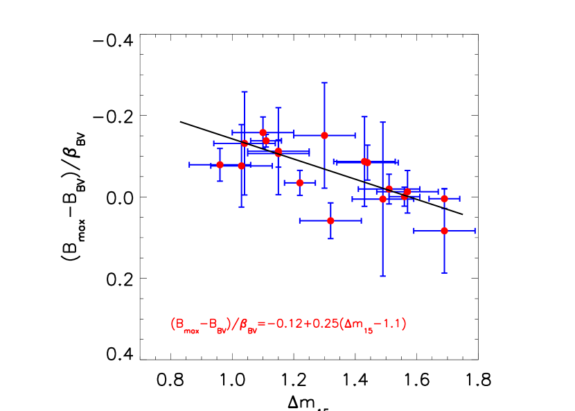
Figure 13: Fits to the $(B_{max}-B_{BV})/\beta_{BV}$ versus $\Delta m_{15}$ relation for a sub-sample of SNe with $(B_{max}-V_{max})$ $\leq$ 0^m.05. The quantity $(B_{max}-B_{BV})/\beta_{BV}$ can be used to estimate the color excess due to extinction.

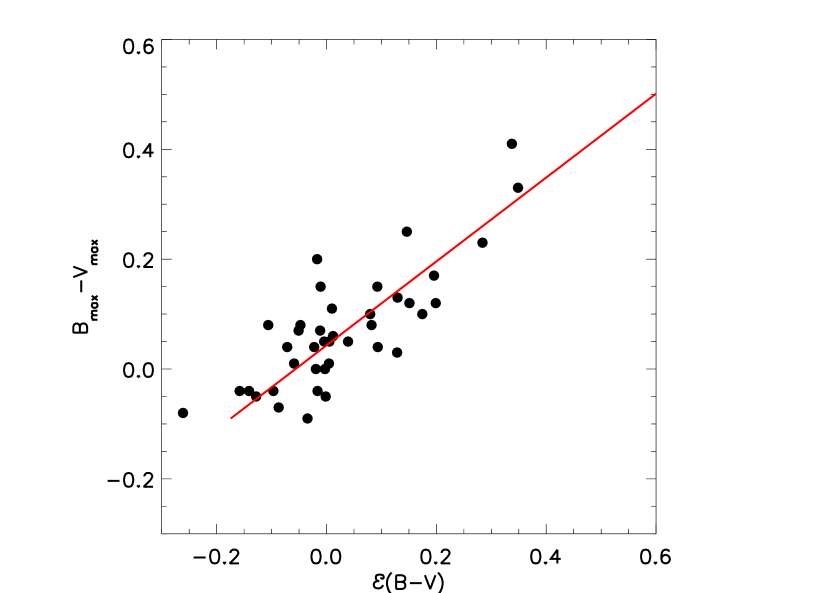
Figure 14: Correlations of ${E}_{BV}(B-V)\ =\ (B_{max}-B_{BV})/\beta_{BV}$ with $(B_{max}-V_{max})$ (a), and E_Ph(B-V) derived by Phillips et al (1999) (b). The Bayesian Prior described in Phillips et al. (1999) is used for both quantities in (b).

Assuming that the above equation represents the $\Delta m_{15}$ dependence of ${\mathcal{E}}_{0}$ for supernovae with negligible extinction, we can derive the color-excesses of any SN Ia using the formula,

$${E}_{BV}(B-V)\ ={\mathcal{E}}(B-V)\ -\ {\mathcal{E}}_{0}.$$

As a consistency check, we also analyzed the correlations between ${\mathcal{E}}(B-V)$ defined in equation (7) and $(B_{max}-V_{max})$. The results are shown in Figure 14(a) for the supernovae with $B_{max}-V_{max}\ <\ 0.5$. The solid line in Figure 14(a) corresponds to

$${\mathcal{E}}(B-V)\ =\ (-0.051\pm 0.011)+(1.000\pm 0.067)(B_{max}-V_{max}).$$

The relation given in equation (10) is interesting because the slope is consistent with 1. This means that ${\mathcal{E}}(B-V)$ is apparently a straightforward alternative to $(B_{max}-V_{max})$ for measuring the color-excess.

To compare with the color-excess $E_{Ph}(B-V)$ deduced by Phillips et al. (1999), we have made use of equation (9) to calculate $E_{BV}(B-V)$ and applied the same Bayesian prior used in Phillips et al. (1999). The estimated color-excess values are shown in Column 9 of Table 1 and in Figure 14(b). The corresponding correlation between the color excesses derived from ${E}_{BV}(B-V)$ and those derived by Phillips et al. (1999) is weaker than the one shown in Figure 14(a) but the values are nonetheless consistent. These are shown in Figure 14(b), where $E_{Ph}(B-V)$ denotes the color-excess derived by Phillips et al. (1999). The Bayesian Prior is so strong here that the correlation in Figure 14(b) becomes less obvious.

It appears that the dispersion of the magnitude at maximum after removing the $\Delta m_{15}$ dependence are comparable for the extinction corrections based on the color-excess derived from equation (9) and for those based on the color-excess of Phillips et al. (1999). The results of the $\Delta m_{15}$ fits are shown as $M^{Bc}_{max}$ in Tables 2, 3, and 4, which should be compared with $M^{B}_{max}$ since they differ only by the extinction estimates. Note also that by definition, applying the color-excess derived from equation (9) to $B_{max}$ and $B_{BV}$ produces identical results.

It is interesting to compare the method outlined in equations 6, 7, 8, and 9 with the method described in Tripp (1997) and Tripp & Branch (1999), in which maximum magnitudes were fitted by $\Delta m_{15}$ and $B_{max}-V_{max}$ simultaneously to account for both intrinsic differences of SN luminosity and extinctions. The dependence on $B_{max}-V_{max}$ has a slope close to 2 in Tripp & Branch (1999). This slope is apparently related to both the intrinsic properties of a supernova and the underlying extinction law which determines $R_{B}$. Phillips et al. (1999) found that a value around $R_{B}\ =\ 3.5$ provides better fits. In fact, we can also leave $R_{B}$ as a free parameter and make joint two parameter fits to $M^{B}_{max}$ versus $\Delta m_{15}$ and ${\mathcal{E}}(B-V)$. The current method will also be able to effectively separate the intrinsic color and the color-excess due to dust extinction, but we will leave these treatments and self-consistent dust extinction estimates for a later paper.

5 Observational Strategies for CMAGIC

It is noteworthy that the CMAGIC method is applicable in cases where the SN is first observed well past maximum light, an epoch at which the extrapolated fit to the light curve maximum becomes questionable. It can also simplify SN Ia observations for distance estimates. There are several strategies that may take advantage of this method, which we describe in order of increasing number of measurements needed on each SN.

First, in the extreme case, a single pair of data points with two color photometry from a color-excess free supernova such as those from E+S0 galaxies may be used to obtain a distance modulus estimate that is accurate to about 0.16 mag even without knowledge of the stretch factor if the co-moving frame $B$ and $V$ filters are used. As shown in §3, systematic errors introduced by assuming a universal $\beta_{BV}$ value are less than $\sim 0^{m}.06$ and more typically $\sim 0^{m}.03$ when $B-V$ is measured within $\pm 0^{m}.2$ of 0${}^{m}.6$. The observations have to be made in the linear regime, typically around day 10-20 so that CMAGIC is applicable. A rough estimate of the epoch and redshift must be obtained independently most likely by using a single spectrum (Riess et al., 1998). This simple method does not provide proper extinction estimates and can be applied only when extinction can be estimated independently. Such sparse data points may be useful for high redshift supernovae where detailed light curves are hard to obtain. This method might be termed the “CMAGIC-Snapshot” method, but should be applied with caution as there is no control of systematics.

A significant improvement is achieved if, in addition to color information around day 10-20, a single-band light curve is also obtained at a certain color that allows for a fit to the maximum magnitude and stretch factor as has been routinely done in current supernova observations. With such a data set, stretch/$\Delta m_{15}$ corrections can be applied, and a color-excess-free estimator can be constructed. It is also practical to estimate dust extinction using the method described above. Such data can be obtained for most of the Type Ia supernovae discovered by modern techniques, from low redshift to redshift as high as $\sim\ 0.85$ from the ground, but space-based observatories are needed to observe supernovae at even higher redshifts in the multiple bands to get extinction (Aldering et al., 2002a, b).

If more color information and light curve information is available, joint fits to stretch/$\Delta m_{15}$ correction and CMAGIC can be attempted to reduce errors on the color-excess free estimator and even absolute extinction $A_{\lambda}$ to achieve unbiased distances. In particular, we have shown that the color magnitude relation is a very robust relation that none of the current standard fitting procedures can match in quality. The Color Magnitudes are less sensitive to errors in extinction corrections. The corrections for light curve shapes are smaller and therefore are less sensitive to errors of $\Delta m_{15}$ or stretch. These properties make CMAGIC a more robust and reliable method for analyzing SN Ia light curves.

6 Discussions and Conclusions

We have presented in this study a new way to analyze photometric data of SN Ia for cosmological distance determinations. Our method is based on post-maximum observations of SN Ia and we find that a precise distance estimate which corrects simultaneously for the $\Delta m_{15}$/stretch relation and color-excess can be obtained with well-sampled light curves in different filters. We have seen that the magnitude of Type Ia SNe at a given color index has a very small dispersion for most of the first month past maximum, and the linear fit in this region is simple and robust for $B$, $V$, $R$, and $I$ data. Working in the color-magnitude plane rather than magnitude- or color-versus-time captures better the homogeniety of SN Ia. It also is less affected by errors in extinction estimates in most bands. Finally it allows a different part of the SN lightcurve to be explored in hunts for new evolutionary parameters. This method may be useful for ground- or space-based multi-color supernova surveys.

CMAGIC emphasizes post maximum data and gives zero weight for data taken outside the linear regime. Compared with other methods, CMAGIC is more transparent and error propagation is more straight forward. The fundamental difference between the CMAGIC approach and other approaches such as stretch fit (Perlmutter et al., 1997), template fit (Pskovskii, 1977; Phillips, 1993), and MLCS (Riess et al., 1996) is that CMAGIC uses the color magnitude plane and particularly the linear relation found for all Type Ia supernovae; it does not employ any template light curves. The differences in input mathematical models determine that CMAGIC is intrinsically different from MLCS. There is no reason to suppose that a linear sequence of time parametrized light curves, such as in MLCS, is guaranteed to capture all variations of Type Ia SNe. In particular, as shown in Figure 6b, the fitting templates of MLCS from Riess et al. (1996) can not reproduce the bump feature on the CMAG diagram which is observed for many intrinsically bright supernovae. (The magnitude dispersion on the Hubble Diagram given in Riess et al. (1996) is generally larger than what we derived from CMAGIC for comparable samples of supernovae.) Future versions of the MLCS, template fitting, or stretch fitting approaches may or may not be able to incorporate the CMAGIC empirical relation, but the current implementations do not.

One important application of the method is to derive color-excesses due to dust extinction. The method discussed in Phillips et al. (1999) which makes use of nebular phase data is hard to apply to faint distant supernovae. The extinction estimate provided in this study can be a useful tool for both high and low redshift supernovae.

Fitting the slope of CMAGIC may come as a handy parameter to probe the progenitor systems. The slope is an observable parameter and we have already seen from Figures 7 and 9 that there is an intrinsic dispersion of the slopes which can not be accounted for by observational errors. Figures 7 and 9 are suggestive that we may have seen a bifurcation of the slope distribution with one branch of SN Ia showing slopes of about $\beta_{BV}\ \sim\ 1.65$ and the other showing about $\beta_{BV}\ \sim\ 2.0$. If this is real, it implies that we may be witnessing some fundamentally different groups of supernovae with different chemical structures or evolutionary paths. These questions will be extremely interesting questions to be addressed by systematic supernova observation programs.

Detailed radiative transfer calculations are needed to understand the CMAGIC relations. A possible key factor for the success of CMAGIC is that the ejecta of Type Ia supernovae are more uniform in the zones of complete nuclear burning which are only visible after maximum light. The CMAGIC relations are determined mostly by the chemical and ionization structures close to the photosphere which for SNe Ia are perhaps more uniform as they lie in regions of complete thermal nuclear reaction (Höflich et al., 1998).

One other line of evidence for this homogeneity just past maximum light comes from polarization studies. Spectropolarimetry of SNe Ia indicate that the supernova photospheres are more asymmetric before and around optical maximum (Wang et al., 1996; Howell et al., 2001; Wang et al., 2002). The value representing the asphericity of the photosphere can be determined to be around 10%, which would introduce dispersions due to view-angle differences of up to 0.1 magnitude before and around optical maximum, but most post maximum observations show non-detectable polarizations down to about 0.2-0.3% (Wang et al., 1996; Wang et al., 2002), indicating that their post maximum behavior can be more uniform than before optical maximum.

The dramatic improvement in magnitude dispersion as implied in Figure 11, if borne out by future nearby supernova observations, would have important impact for the use of Type Ia supernovae as cosmological distance indicators.

Appendix A The Complete Set of Magnitude versus Color plots

We show in Figures A1, A2, and A3 the color-magnitude plots for B-V, B-R, and B-I colors, respectively. All these Figures represent the magnitudes and colors as measured with no extinction or $K$-corrections. Linear regimes can be identified for all the colors.

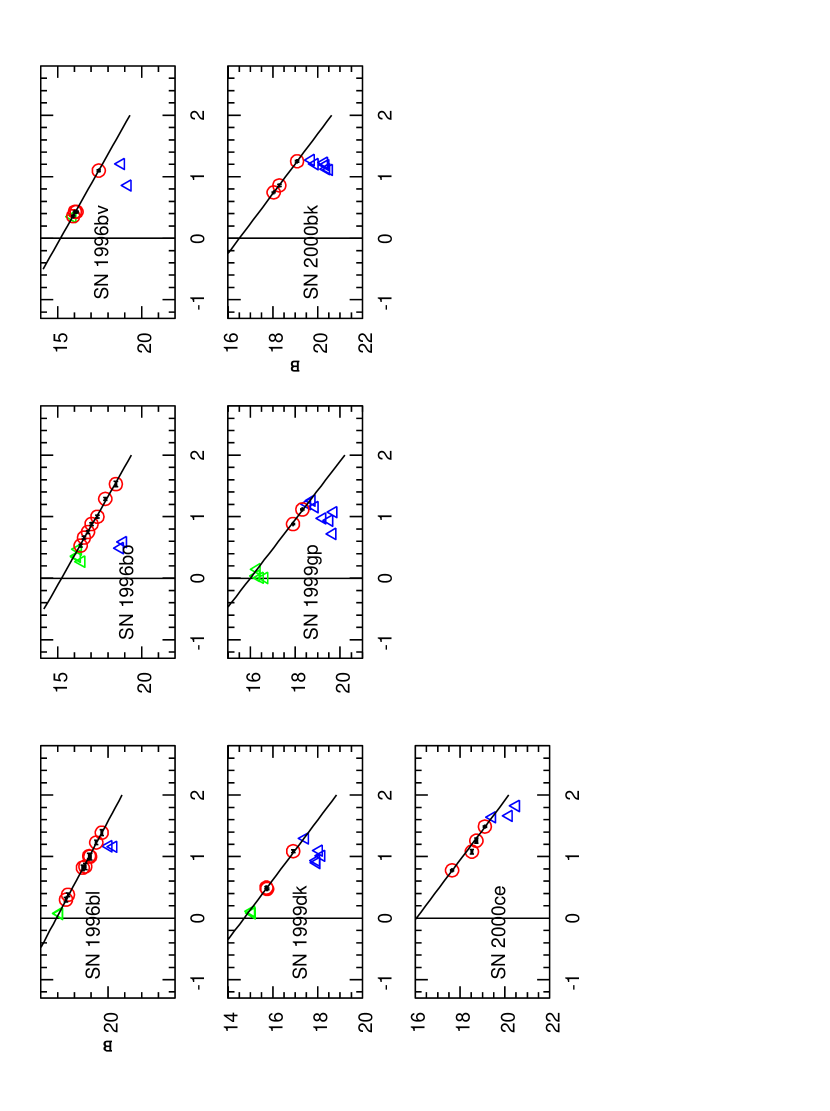
Figure A1: Observed B magnitude versus B-V for the sample of well observed SNe (Hamuy et al. 1996; Riess et al. 1999; Krisciunas et al. 2001). The linear fits are shown in solid lines. The data points used for the linear fits are shown as red circles. The green triangles show data points before the linear region, and the blue triangles show data after the linear region.

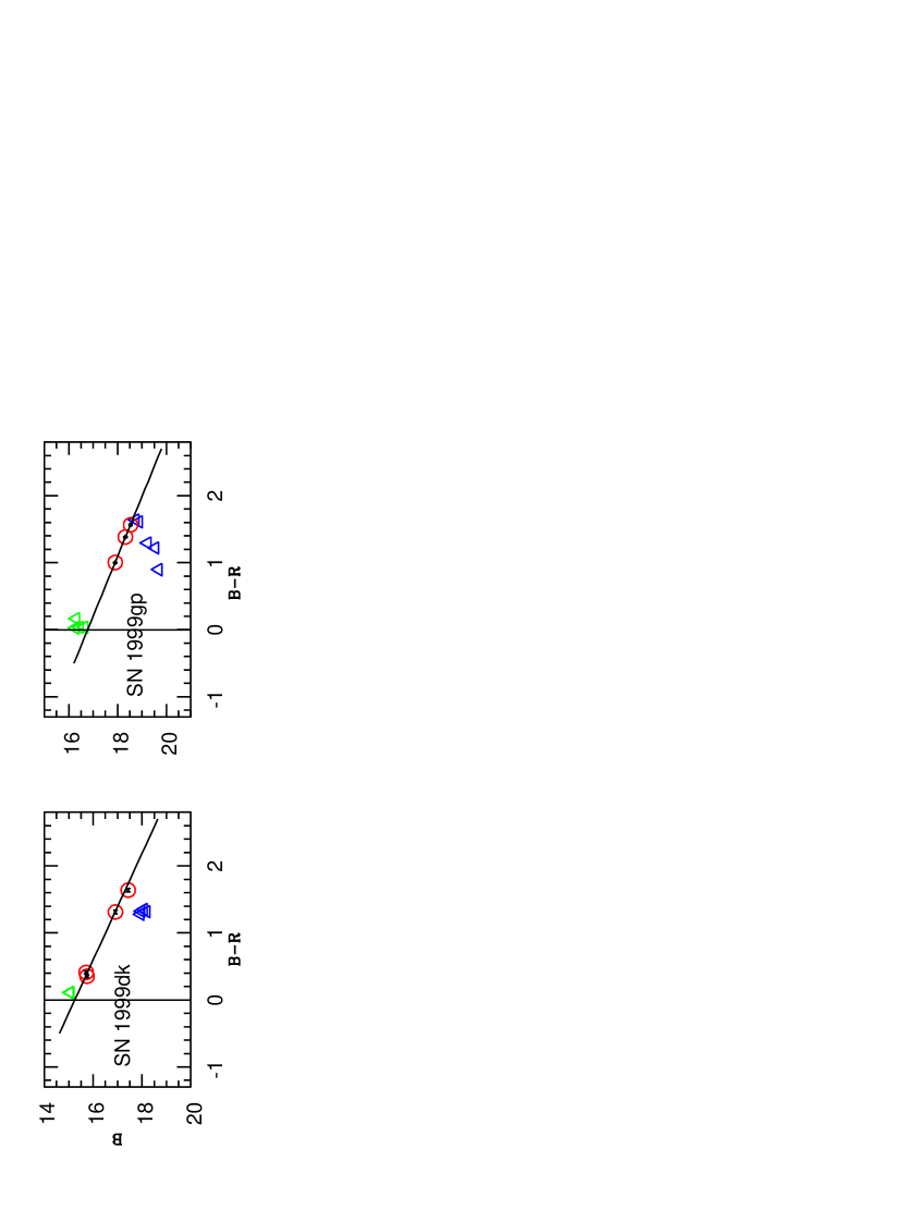
Figure A2: Same as Fig. 1, but for B versus B-R.

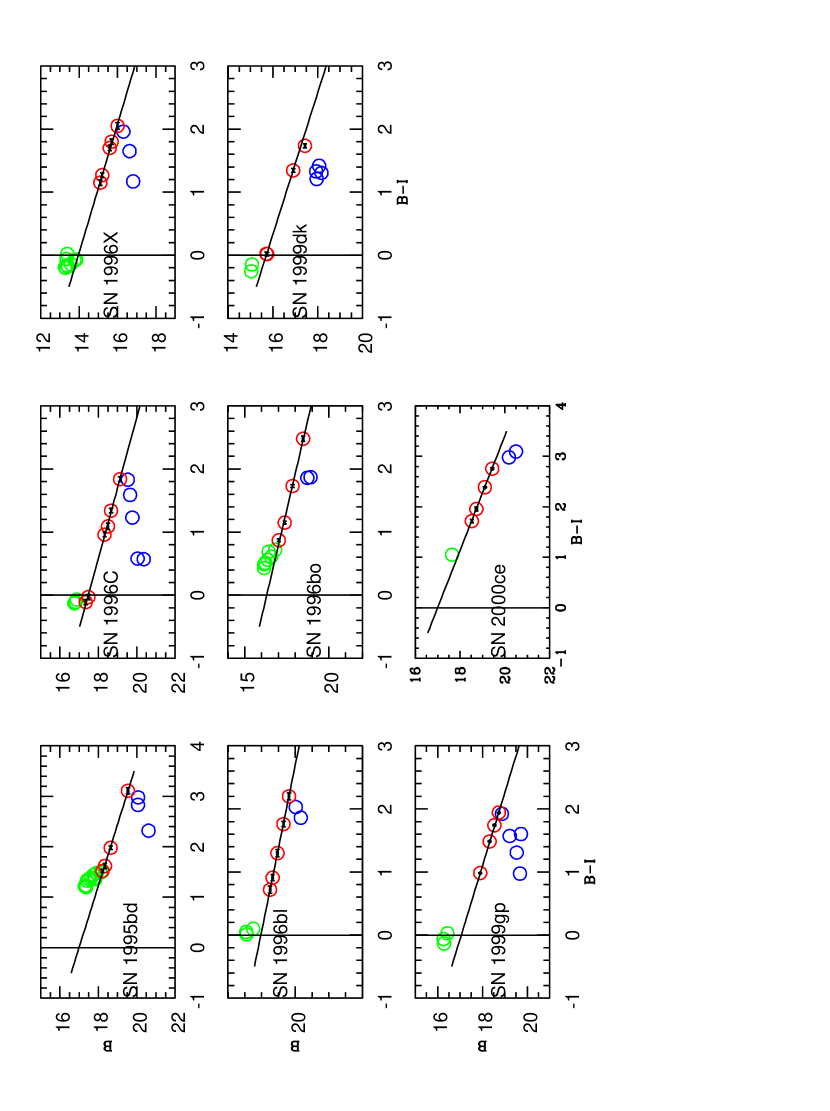
Figure A3: Same as Fig. 1, but for B versus B-I.

References

- Aldering et al. (2002a) Aldering, G., Supernova Cosmology Project Collaboration, & Nearby Supernova Factory Collaboration. 2002, SPIE, in press
- Aldering et al. (2002b) Aldering, G., SNAP Collaboration 2002, SPIE, in press
- Cardelli et al. (1989) Cardelli, J. A., Clayton, G. C., & Mathis, J. S. 1989, ApJ, 345, 245
- Filippenko & Leonard (1995) Filippenko, A. V. & Leonard, D. C. 1995, IAU Circ., 6237, 2
- Garnavich et al. (1995) Garnavich, P., Riess, A., Kirshner, R., & Berlind, P. 1995, IAU Circ., 6278, 1
- Garnavich et al. (2001) Garnavich, P. M., Bonanos, A. Z., Jha, S., Kirshner, R. P., Schlegel, E. M., Challis, P., Macri, L. M., Hatano, K., Branch, D., Bothun, G. D., & Freedman, W. L. 2001, in 28 preprint pages including 17 figures. Submitted to ApJ. High-resolution version available from http://www.nd.edu/ pgarnavi/sn99by/sn99by.ps, 5490
- Goldhaber et al. (2001) Goldhaber, G., Groom, D. E., Kim, A., Aldering, G., Astier, P., Conley, A., Deustua, S. E., Ellis, R., Fabbro, S., Fruchter, A. S., Goobar, A., Hook, I., Irwin, M., Kim, M., Knop, R. A., Lidman, C., McMahon, R., Nugent, P. E., Pain, R., Panagia, N., Pennypacker, C. R., Perlmutter, S., Ruiz-Lapuente, P., Schaefer, B., Walton, N. A., & York, T. 2001, ApJ, 558, 359
- Hamuy et al. (1994) Hamuy, M., Philips, M. M., Maza, J., Suntzeff, N. B., della Valle, M., Danziger, J., Antezana, R., Wischnjwesky, M., Aviles, R., Schommer, R. A., Kim, Y.-C., Wells, L. A., Ruiz, M. T., Prosser, C. F., Krzeminski, W., Baylin, C. D., Hartigan, P., & Hughes, J. 1994, AJ, 108, 2226
- Hamuy et al. (1996a) Hamuy, M., Phillips, M. M., Suntzeff, N. B., Schommer, R. A., Maza, J., Antezan, A. R., Wischnjewsky, M., Valladares, G., Muena, C., Gonzales, L. E., Aviles, R., Wells, L. A., Smith, R. C., Navarrete, M., Covarrubias, R., Williger, G. M., Walker, A. R., Layden, A. C., Elias, J. H., Baldwin, J. A., Hernandez, M., Tirado, H., Ugarte, P., Elston, R., Saavedra, N., Barrientos, F., Costa, E., Lira, P., Ruiz, M. T., Anguita, C., Gomez, X., Ortiz, P., della Valle, M., Danziger, J., Storm, J., Kim, Y.-C., Bailyn, C., Rubenstein, E. P., Tucker, D., Cersosimo, S., Mendez, R. A., Siciliano, L., Sherry, W., Chaboyer, B., Koopmann, R. A., Geisler, D., Sarajedini, A., Dey, A., Tyson, N., Rich, R. M., Gal, R., Lamontagne, R., Caldwell, N., Guhathakurta, P., Phillips, A. C., Szkody, P., Prosser, C., Ho, L. C., McMahan, R., Baggley, G., Cheng, K.-P., Havlen, R., Wakamatsu, K., Janes, K., Malkan, M., Baganoff, F., Seitzer, P., Shara, M., Sturch, C., Hesser, J., Hartig, A. N. P., Hughes, J., Welch, D., Williams, T. B., Ferguson, H., Francis, P. J., French, L., Bolte, M., Roth, J., Odewahn, S., Howell, S., & Krzeminski, W. 1996a, AJ, 112, 2408
- Hamuy et al. (1996b) Hamuy, M., Phillips, M. M., Suntzeff, N. B., Schommer, R. A., Maza, J., Smith, R. C., Lira, P., & Aviles, R. 1996b, AJ, 112, 2438
- Hamuy et al. (1993) Hamuy, M., Phillips, M. M., Wells, L. A., & Maza, J. 1993, PASP, 105, 787
- Höflich et al. (1998) Höflich, P., Wheeler, J. C., & Thielemann, F. K. 1998, ApJ, 495, 617
- Howell et al. (2001) Howell, D. A., Höflich, P., Wang, L., & Wheeler, J. C. 2001, ApJ, 556, 302
- Kim et al. (1996) Kim, A., Goobar, A., & Perlmutter, S. 1996, PASP, 108, 190
- Krisciunas et al. (2001) Krisciunas, K., Phillips, M. M., Stubbs, C., Rest, A., Miknaitis, G., Riess, A. G., Suntzeff, N. B., Roth, M., Persson, S. E., & Freedman, W. L. 2001, AJ, 122, 1616
- Leibundgut (1988) Leibundgut, B. 1988, Ph.D. Thesis, 171
- Li et al. (2001) Li, W., Filippenko, A. V., Gates, E., Chornock, R., Gal-Yam, A., Ofek, E. O., Leonard, D. C., Modjaz, M., Rich, R. M., Riess, A. G., & Treffers, R. R. 2001, PASP, 113, 1178
- Li et al. (1999) Li, W. D., Qiu, Y. L., Qiao, Q. Y., Zhu, X. H., Hu, J. Y., Richmond, M. W., Filippenko, A. V., Treffers, R. R., Peng, C. Y., & Leonard, D. C. 1999, AJ, 117, 2709
- Lira (1995) Lira, P. 1995, Masters thesis, Univ. Chile
- Nugent & et al. (2002) Nugent, P. & et al. 2002, ApJ, submitted
- Oke & Sandage (1968) Oke, J. B. & Sandage, A. 1968, ApJ, 154, 21
- Pavlyuk et al. (1998) Pavlyuk, N. N., Tsvetkov, D. Y., Pskovskii, Y. P., & Bartunov, O. S. 1998, Astronomy Letters, 24, 826
- Perlmutter et al. (1999) Perlmutter, S., Aldering, G., Goldhaber, G., Knop, R. A., Nugent, P., Castro, P. G., Deustua, S., Fabbro, S., Goobar, A., Groom, D. E., Hook, I. M., Kim, A. G., Kim, M. Y., Lee, J. C., Nunes, N. J., Pain, R., Pennypacker, C. R., Quimby, R., Lidman, C., Ellis, R. S., Irwin, M., McMahon, R. G., Ruiz-Lapuente, P., Walton, N., Schaefer, B., Boyle, B. J., Filippenko, A. V., Matheson, T., Fruchter, A. S., Panagia, N., Newberg, H. J. M., Couch, W. J., & The Supernova Cosmology Project. 1999, ApJ, 517, 565
- Perlmutter et al. (1997) Perlmutter, S., Gabi, S., Goldhaber, G., Goobar, A., Groom, D. E., Hook, I. M., Kim, A. G., Kim, M. Y., Lee, J. C., Pain, R., Pennypacker, C. R., Small, I. A., Ellis, R. S., McMahon, R. G., Boyle, B. J., Bunclark, P. S., Carter, D., Irwin, M. J., Glazebrook, K., Newberg, H. J. M., Filippenko, A. V., Matheson, T., Dopita, M., Couch, W. J., & The Supernova Cosmology Project. 1997, ApJ, 483, 565
- Phillips (1993) Phillips, M. M. 1993, ApJ, 413, L105
- Phillips et al. (1999) Phillips, M. M., Lira, P., Suntzeff, N. B., Schommer, R. A., Hamuy, M., & Maza, J. . 1999, AJ, 118, 1766
- Pskovskii (1977) Pskovskii, I. P. 1977, Soviet Astronomy, 21, 675
- Pskovskii (1984) Pskovskii, I. P. 1984, Soviet Astronomy, 28, 658
- Riess et al. (1999) Riess, A. G., Kirshner, R. P., Schmidt, B. P., Jha, S., Challis, P., Garnavich, P. M., Esin, A. A., Carpenter, C., Grashius, R., Schild, R. E., Berlind, P. L., Huchra, J. P., Prosser, C. F., Falco, E. E., Benson, P. J., Briceño, C. ., Brown, W. R., Caldwell, N., dell’Antonio, I. P., Filippenko, A. V., Goodman, A. A., Grogin, N. A., Groner, T., Hughes, J. P., Green, P. J., Jansen, R. A., Kleyna, J. T., Luu, J. X., Macri, L. M., McLeod, B. A., McLeod, K. K., McNamara, B. R., McLean, B., Milone, A. A. E., Mohr, J. J., Moraru, D., Peng, C., Peters, J., Prestwich, A. H., Stanek, K. Z., Szentgyorgyi, A., & Zhao, P. 1999, AJ, 117, 707
- Riess et al. (1998) Riess, A. G., Nugent, P., Filippenko, A. V., Kirshner, R. P., & Perlmutter, S. 1998, ApJ, 504, 935
- Riess et al. (1996) Riess, A. G., Press, W. H., & Kirshner, R. P. 1996, ApJ, 473, 88
- Tripp (1997) Tripp, R. 1997, A&A, 325, 871
- Tripp & Branch (1999) Tripp, R. & Branch, D. 1999, ApJ, 525, 209
- Wang et al. (1997) Wang, L., Hoeflich, P., & Wheeler, J. C. 1997, ApJ, 483, L29
- Wang et al. (2001) Wang, L., Kasen, D. N., Baade, D., Fransson, C., Howell, D. A., Hoeflich, P., Lundqvist, P., Nugent, P. E., & Wheeler, J. C. 2001, IAU Circ., 7724, 2
- Wang et al. (1996) Wang, L., Wheeler, J. C., Li, Z., & Clocchiatti, A. 1996, ApJ, 467, 435
- Wang et al. (2002) Wang, L., et al., 2002, ApJ, submitted