‘Thermal’ SiO radio line emission towards M-type AGB stars:
a probe of circumstellar dust formation and dynamics

An extensive radiative transfer analysis of circumstellar SiO ‘thermal’ radio line emission from a large sample of M-type AGB stars has been performed. The sample contains 18 irregulars of type Lb (IRV), 7 and 34 semiregulars of type SRa and SRb (SRV), respectively, and 12 Miras. New observational data, which contain spectra of several ground vibrational state SiO rotational lines, are presented. The detection rate was about 60% (44% for the IRVs, and 68% for the SRVs). SiO fractional abundances have been determined through radiative transfer modelling. The abundance distribution of the IRV/SRV sample has a median value of 6$\times$10^-6, and a minimum of 2$\times$10^-6 and a maximum of 5$\times$10^-5. The high mass-loss rate Miras have a much lower median abundance, $\lesssim$10^-6. The derived SiO abundances are in all cases well below the abundance expected from stellar atmosphere equilibrium chemistry, on average by a factor of ten. In addition, there is a trend of decreasing SiO abundance with increasing mass-loss rate. This is interpreted in terms of depletion of SiO molecules by the formation of silicate grains in the circumstellar envelopes, with an efficiency which is high already at low mass-loss rates and which increases with the mass-loss rate. The high mass-loss rate Miras appear to have a bimodal SiO abundance distribution, a low abundance group (on average 4$\times$10^-7) and a high abundance group (on average 5$\times$10^-6). The estimated SiO envelope sizes agree well with the estimated SiO photodissociation radii using an unshielded photodissociation rate of 2.5 $\times$ 10^-10 s^-1. The SiO and CO radio line profiles differ in shape. In general, the SiO line profiles are narrower than the CO line profiles, but they have low-intensity wings which cover the full velocity range of the CO line profile. This is interpreted as partly an effect of selfabsorption in the SiO lines, and partly (as has been done also by others) as due to the influence of gas acceleration in the region which produces a significant fraction of the SiO line emission. Finally, a number of sources which have peculiar CO line profiles are discussed from the point of view of their SiO line properties.

1 Introduction

The atmospheres of and the circumstellar envelopes (CSEs) around Asymptotic Giant Branch (AGB) stars are regions where many different molecular species and dust grains form efficiently. The molecular and grain type setups are to a large extent determined by the C/O-ratio of the central star. For instance, SiO is formed in the extended atmospheres of both M-type [C/O$<$1; O-rich] and C-type [C/O$>$1] AGB stars, but its abundance is much higher in the former. Therefore, the SiO ‘thermal’ line emission (i.e., rotational lines in the $v$=0 state; the term ‘thermal’ is used here to distinguish the $v$=0 state emission from the strong maser line emission from vibrationally excited states) is particularly strong towards M-stars, with the intensity of e.g. the $J$=2$\rightarrow$1 line comparable to, or even stronger than, that of the CO $J$=1$\rightarrow$0 emission. Nevertheless, the initial observations of SiO thermal radio line emission from AGB-CSEs (Lambert & Vanden Bout, 1978; Wolff & Carlson, 1982) and their interpretation (Morris et al., 1979) suggested circumstellar SiO abundances (several) orders of magnitude lower than those expected from the chemical equilibrium models (Tsuji, 1973).

Over the years the observational basis has improved considerably (Bujarrabal et al., 1986, 1989; Bieging & Latter, 1994; Bieging et al., 1998, 2000; Olofsson et al., 1998), and even some interferometer data exist (Lucas et al., 1992; Sahai & Bieging, 1993). These data suggest that the SiO line emission originates in two regions, one close to the star with a high SiO abundance, and one extended region with a low SiO abundance. The relative contributions to the SiO line emission from these two regions depend on the mass-loss rate.

This structure has been interpreted as due to accretion of SiO onto dust grains (Bujarrabal et al., 1989; Sahai & Bieging, 1993). After the grains nucleate near the stars, they grow in part because of adsorption of gas-phase species. In O-rich CSEs, refractory elements like Si, together with O, are very likely the main constituents of the grains, which are identified through the 9 and 18 $\mu$m silicate features in the infrared spectra of the stars (Forrest et al., 1975; Pégourié & Papoular, 1985). Therefore, molecules like SiO are expected to be easily incorporated into the dust grains. As a result, the SiO gas phase abundance should fall off with increasing distance from the star as SiO molecules in the outflowing stellar wind are incorporated into the grains. The depletion process is, however, quite uncertain since it does not proceed at thermal equilibrium. Eventually, photodissociation destroys all of the remaining SiO molecules.

The grain formation is important not only for the chemical composition of the CSE, but also because it affects its dynamical state [the radiation pressure acts on the grains which are dynamically coupled to the gas, e.g., Kwok (1975)]. The SiO radio line profiles are narrower than those of CO and have mostly Gaussian-like shapes (e.g., Bujarrabal et al. (1986, 1989)), a fact suggesting that the SiO line emission stems from the inner regions of the CSEs, where grain formation is not yet complete and where the stellar wind has not reached its terminal expansion velocity. This result is corroborated by interferometric observations which show that the size of the SiO line emitting region is independent of the line-of-sight velocity (Lucas et al., 1992). Lucas et al. explained this as a result of a rather extended acceleration region. However, Sahai & Bieging (1993), using a more detailed modelling, were able to explain both the line profiles and the brightness distributions with a ‘normal’ CSE, i.e., with a rather high initial acceleration.

Therefore, ‘thermal’ SiO radio line emission is a useful probe of the formation and evolution of dust grains in CSEs, a complex phenomenon that is yet not fully understood, as well as the CSE dynamics.

In this paper we present a detailed study of SiO radio line emission from the CSEs of a sample of M-type AGB stars. The sample includes irregular (IRVs), semiregular (SRVs) and Mira (M) variables. The IRVs and SRVs have already been studied in circumstellar CO radio line emission (Olofsson et al., 2002), yielding estimates of the stellar mass-loss rates. Using these estimates a radiative transfer modelling of the SiO radio line emission is performed. A complete analysis of the circumstellar CO and SiO line emission is done for the Mira sub-sample.

2 Observations of the IRV/SRV sample

2.1 The IRV/SRV sample

The sample contains all the M-type IRVs and SRVs detected in circumstellar CO radio line emission by Kerschbaum & Olofsson (1999) and Olofsson et al. (2002). The original source selection criteria are described in Kerschbaum & Olofsson (1999), but basically these stars are the brightest 60 $\mu$m-sources (IRAS $S_{60}$ typically above 3 Jy, with IRAS quality flag 3 in the 12, 25, and 60 $\mu$m bands) that appear as IRVs or SRVs in the General Catalogue of Variable Stars [GCVS4; Kholopov (1990)]. The detection rate of circumstellar CO was rather high, about 60% (Olofsson et al. (2002); 69 stars detected). The basic properties of the stars are listed in Kerschbaum & Olofsson (1999) and Olofsson et al. (2002).

The distances, presented in Table 4, were derived using an assumed bolometric luminosity of 4000 L_⊙ for all stars. We are aware of the fact that such a distance estimate have a rather large uncertainty for an individual object but it is adequate for a statistical study of a sample of stars (see discussion by Olofsson et al. (2002)). The apparent bolometric fluxes were obtained by integrating the spectral energy distributions ranging from the visual data over the near-infrared to the IRAS-range (Kerschbaum & Hron, 1996).

2.2 The observing runs

The SiO ($v$=0, $J$=2$\rightarrow$1; hereafter all SiO transitions are in the ground vibrational state) data were obtained using the 20 m telescope at Onsala Space Observatory (OSO) and the 15 m Swedish-ESO Submillimetre Telescope (SEST) on La Silla, Chile. At SEST, a sizable fraction of the stars were observed also in the SiO $J$=3$\rightarrow$2 line, and four additional sources were observed with the IRAM 30 m telescope at Pico Veleta, Spain, in this line. The higher-frequency lines, $J$=5$\rightarrow$4 and 6$\rightarrow$5, were observed towards 10 and 3 stars, respectively. The observing runs at OSO were made over the years 1993 to 2000, at SEST over the years 1992 to 2003, and at IRAM between October 18 and 22 in 1997. Telescope and receiver data are given in Table 1. $T_{\rm rec}$ and $\eta_{\rm mb}$ stand for the representative noise temperature of the receiver (SSB) and the main beam efficiency of the telescope, respectively.

Two filterbanks at OSO (256$\times$250 kHz, and 512$\times$1 MHz), two acousto-optical spectrometers at SEST (86 MHz bandwidth with 43 kHz channel separation, and 1 GHz bandwidth with 0.7 MHz channel separation), and a 1 MHz filter bank at IRAM were used as spectrometers. Dual beam switching (beam throws of about 11′), in which the source was placed alternately in the two beams, was used to eliminate baseline ripples at OSO and SEST, while a wobbler switching with a throw of 150$\arcsec$ in azimuth was used at IRAM. Pointing and focussing were checked every few hours. The line intensities are given in the main beam brightness temperature scale ($T_{\rm mb}$), i.e., the antenna temperature has been corrected for the atmospheric attenuation (using the chopper wheel method) and divided by the main beam efficiency.

Table 1: Data on telescopes and receivers

Telescope Frequency Beamwidth $$T_{\rm rec}$$

[MHz] [] [K]

OSO 86847 42 150 0.55

SEST 86847 57 100 0.75

SEST 130269 39 120 0.65

IRAM 130269 18 150 0.58

SEST 217105 25 600 0.55

SEST 260518 21 800 0.45

2.3 Observational results

A total of 60 stars were observed in circumstellar SiO line emission (i.e., about 85% of the stars detected in circumstellar CO): 34 stars were detected in the SiO $J$=2$\rightarrow$1 line, 21 in the $J$=3$\rightarrow$2 line, and 3 in the $J$=5$\rightarrow$4 and $J$=6$\rightarrow$5 lines. Clear detections of SiO lines were obtained towards 36 sources, i.e., the detection rate was about 60%: 8 IRVs (detection rate 44%) and 28 SRVs (detection rate 68%) were detected. Tables 6 and 7 in the Appendix list all our SiO observations. The names in the GCVS4 and the IRAS-PSC are given. The first letter of the code denotes the observatory (IRAM, OSO, or SEST), the rest the transition observed. Another code reflects the ‘success’ of the observation (Detection, Non-detection).

The stellar velocity is given with respect to the heliocentric ($v_{\rm hel}$) and LSR frame [$v_{\rm LSR}$; the Local Standard of Rest is defined using the standard solar motion (B1950.0): $v_{\odot}$= 20 km s^-1, $\alpha_{\odot}$= 270.5^∘, $\delta_{\odot}$= +30^∘]. The stellar velocity, the expansion velocity, and the main beam brightness temperature were obtained by fitting the function $T_{\rm mb}[1-((v_{*}-v_{\rm z})/v_{\rm e})^{2}]^{\gamma}$ to the line profile. The integrated intensity, $I$= $\int T_{\rm mb}$ $dv$, is obtained by integrating the line intensities over the line profile. The uncertainty in $I$ varies with the S/N-ratio, but we estimate that it is on avarage $<$15%. To this should be added an estimated uncertainty in the absolute calibration of about 20%. For a non-detection an upper limit to $I$ is estimated by measuring the peak-to-peak noise ($T_{\rm pp}$) of the spectrum with a velocity resolution reduced to 15 km s^-1 and calculating $I$ = 15$T_{\rm pp}$. The Q-column gives a quality ranking: 5 (not detected), 4 (detection with very low S/N-ratio $\lesssim$3), 3 (detection, low S/N-ratio $\approx$5), 2 (detection, good S/N-ratio $\approx$ 10), and 1 (detection, very good S/N-ratio $\gtrsim$15). Finally, in cases of complex velocity profiles the measured component is indicated in the form b=broad, n=narrow, b+n=total.

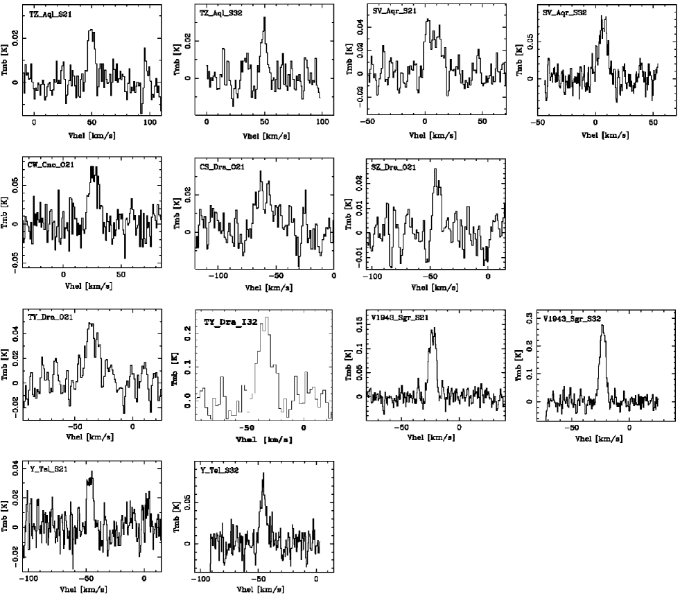
Figure 9: SiO spectra of M-type IRVs. Note the heliocentric velocity scale

All the spectra are shown in Figs. 9 to 12. The velocity scale is given in the heliocentric system. The velocity resolution is reduced to 0.5 km s^-1, except for some low S/N-ratio spectra where a resolution of 1 km s^-1, or even 2 km s^-1, is used, and for some low expansion velocity sources for which 0.25 km s^-1 is used.

3 The Mira sample

In order to make a more extensive study of circumstellar SiO line emission in the CSEs of M-type AGB-stars, a sample of 12 Mira variables with higher mass-loss rates was added. The distances are obtained using the period–luminosity relation of Whitelock et al. (1994). Through modelling of their circumstellar CO radio line emission (Sect. 5), we determined that 4 of the Miras have very high mass-loss rates ($\gtrsim$ 10^-5 M_⊙ yr^-1), 6 are intermediate to high mass loss rate objects ($\gtrsim$ 10^-6 M_⊙ yr^-1) and 2 are low mass-loss rate sources (a few 10^-7 M_⊙ yr^-1).

For this sample data has been gathered from a number of sources. The CO($J$=1$\rightarrow$0) data were taken from Olofsson et al. (1998), while the CO($J$=2$\rightarrow$1, $J$=3$\rightarrow$2, and $J$=4$\rightarrow$3) data were obtained from the archive of the James Clerk Maxwell Telescope on Mauna Kea, Hawaii. The JCMT data are taken at face value after converting to the main beam brightness scale. However, in the cases where there are more than one observation available, the derived line intensities are generally consistent within $\pm$20% (as was found also by Schöier & Olofsson (2001)). The SiO($J$=2$\rightarrow$1) data were obtained from Olofsson et al. (1998). The SiO $J$=5$\rightarrow$4 line was observed in four objects, and the $J$=6$\rightarrow$5 line in one object using SEST with the same observational equipment and procedure as described above.

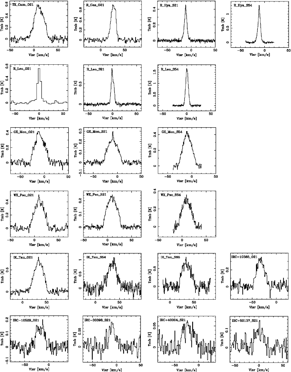
Figure 13: SiO spectra of M-type Miras. Note the LSR velocity scale

The relevant observational results are summarized in Table 8, and the SiO spectra are shown in Fig. 13. The names in the GCVS4 and the IRAS-PSC are given. The first letter of the code denotes the observatory (JCMT, OSO, or SEST), the rest the transition observed.

4 Modelling of circumstellar line emission

Apart from presenting new observational results on thermal SiO radio line emission from AGB-CSEs a rather detailed modelling of the emission will be performed. In some senses this is a more difficult enterprise than the CO line modelling. The SiO line emission predominantly comes from a region closer to the star than does the CO line emission, and this is a region where the observational constraints are poor. The SiO excitation is also normally far from thermal equilibrium with the gas kinetic temperature, and radiative excitation plays a larger role (hence the term ‘thermal’ is really not appropriate). Finally, there exists no detailed chemical model for calculating the radial SiO abundance distribution. These effects make the SiO line modelling much more uncertain, and dependent on a number of assumptions.

The aim is to investigate to what extent the thermal SiO line emission is a useful probe of e.g. the dust formation and the CSE dynamics. There are observational indications that this is the case but the interpretation is normally not straightforward. As an example, Olofsson et al. (1998) found that the line intensity ratio $I$(SiO,$J$=2$\rightarrow$1)/$I$(CO,$J$=1$\rightarrow$0) decreases markedly as a function of a mass-loss rate measure. Their results are reproduced here, but now including all stars of our IRV/SRV and Mira samples, Fig. 1. A straightforward interpretation would be that the SiO abundance decreases with mass-loss rate due to increased depletion efficiency and hence this limits severely the SiO line strength. However, excitation may play an important role here, both for SiO and CO, and a detailed modelling is required.

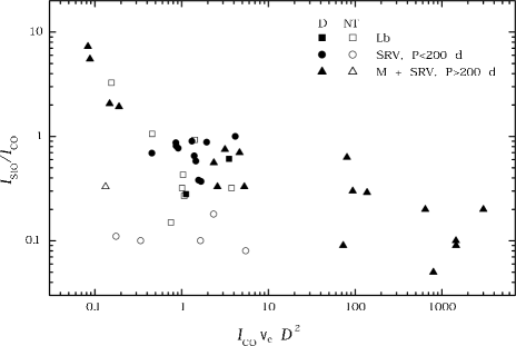
Figure 1: The line intensity ratio $I$(SiO,$J$=2$\rightarrow$1)/$I$(CO,$J$=1$\rightarrow$0) as a function of a mass-loss rate measure [detections are shown as filled symbols, while tentative and negative results are shown as open symbols; see Olofsson et al. (1998)) for more details]

4.1 The method

In order to model the circumstellar SiO line emission a non-LTE radiative transfer code based on the Monte Carlo method has been used (Bernes, 1979). It has been previously used to model circumstellar CO radio line emission in samples of both C- (Schöier & Olofsson, 2000, 2001; Schöier et al., 2002) and O-rich (Olofsson et al., 2002) AGB-CSEs, and also to model the HCN and CN line emission from a limited number of C-rich AGB-CSEs (Lindqvist et al., 2000).

4.2 The SiO molecule

In the excitation analysis of SiO 50 rotational levels in both the ground and the first excited vibrational state are considered. The energy levels of this linear rotor are calculated using the molecular constants from Mollaaghababa et al. (1991). The radiative rates are calculated using the dipole moment from Raymonda et al. (1970). Collisional deexcitation rates have been calculated by Turner et al. (1992)) in the temperature range 20–300 K and up to $J$$=$20. The original data set has been extrapolated in temperature and to include levels up to $J$$=$50 (Schöier et al., in prep.).

4.3 The circumstellar model

The CSEs around AGB-stars are intricate systems where an interplay between different chemical and physical processes takes place. This makes the modelling of circumstellar radio line emission a quite elaborate task. In the analysis presented here, a relatively simple, yet realistic, model for the geometry and kinematics of the CSEs has been adopted. Below follows a short description of the main features of the circumstellar model. For more details we refer to Schöier & Olofsson (2001) and Olofsson et al. (2002).

A spherically symmetric geometry of the CSE is adopted. The mass loss is assumed to be isotropic and constant with time. The gas expansion velocity is assumed to be constant with radius. There is a possibility that neither the mass-loss rate nor the expansion velocity are constant in the regions of interest here. This should be kept in mind when interpreting the results. There is growing evidence for mass-loss modulations of AGB-stars on a time scale of about 1000 yr (Mauron & Huggins, 2000; Marengo et al., 2001; Fong et al., 2003), and the CO line emission comes from a much larger region than that of the SiO lines, and hence averages over a longer time span. Furthermore, the SiO line emission comes from the inner part of the CSE, where it is likely that the gas has not fully reached the terminal velocity. We have not allowed for the presence of gas acceleration nor a time-variable mass loss in the modelling in order to limit the number of free parameters.

The inner boundary of the CSE was set to 1 $\times$ 10¹⁴ cm ($\approx$3R_∗). This parameter is specially important in the case of SiO where radiative excitation is expected to play a role. A turbulent velocity of 0.5 km s^-1 is assumed throughout the entire CSE (see discussion by Olofsson et al. (2002)). The outer boundaries of the molecular abundance distributions are, for both CO and SiO, determined by photodissociation due to the interstellar UV radiation field. For CO we use the modelling of Mamon et al. (1988). The procedure for SiO is presented in Sect. 6.

The radiation field is provided by two sources. The central radiation emanates from the star. This radiation was estimated from a fit to the spectral energy distribution (SED) by assuming two blackbodies, one representing the direct stellar radiation and one the dust-processed radiation (Kerschbaum & Hron, 1996). In the case of optically thin dust CSEs the stellar blackbody temperature derived in this manner is generally about 500 K lower than the effective temperature of the star. The dust mass-loss rates of the IRV/SRVs are low enough that the dust blackbody can be ignored. For the sample of Mira variables both blackbodies were used, since for these high mass-loss rate stars, the excitation of the SiO molecules may be affected by dust emission. The second radiation field is provided by the cosmic microwave bakground radiation at 2.7 K.

In the SiO line modelling the gas kinetic temperature law derived in the modelling of the circumstellar CO radio line emission was used. This is reasonable since the SiO line emission contributes very little to the cooling of the gas. However, the SiO line emission comes mainly from the inner CSE, where the CO lines do not put strong constraints on the temperature, and where other coolants, specifically H₂O, may be important. We estimate though that the kinetic tempartures used in our modelling are not seriously wrong. In addition, for at least the lower mass-loss rates the SiO molecule is mainly radiatively excited, and hence the exact gas kinetic temperature law and the collisional rate coefficients play only a minor role, see Sect. 4.4.

In Sect. 4.4 some implications of these assumptions are discussed.

The mass-loss rates for the sample of IRV/SRVs were already presented in Olofsson et al. (2002). They were derived through modelling of circumstellar CO radio line observations. A median mass loss rate of 2$\times$10^-7 M_⊙ yr^-1 was found for this sample. These mass-loss rate estimates are expected to be accurate to within a factor of a few for an individual object. Nevertheless, they are probably the best mass-loss rate estimates for these types of objects [also in agreement with the mass-loss rate estimates by Knapp et al. (1998) for five sources in common].

The modelling of the circumstellar CO radio line emission for the Mira sample is presented in this paper. The same approach as in Olofsson et al. (2002) has been used, i.e., the energy balance equation is solved simultaneously with the CO excitation. A number of (uncertain) parameters describing the dust are introduced. They are grouped in a global parameter, the $h$-parameter, which is given by

$$h=\left[\frac{\psi}{0.01}\right]\left[\frac{2.0\,\mathrm{g\,cm}^{-3}}{\rho_{\mathrm{gr}}}\right]\left[\frac{0.05\,\mu\mbox{m}}{a_{\mathrm{gr}}}\right],$$ (1)

where $\psi$ is the dust-to-gas mass ratio, $\rho_{\mathrm{gr}}$ the dust grain density, and $a_{\mathrm{gr}}$ its radius. This parameter is particularly important for the heating due to gas-grain collisions. The normalized values are the ones used to fit the CO radio line emission of IRC+10216 using this model Schöier & Olofsson (2001), i.e., $h$=1 for this object. Schöier & Olofsson (2001) found that on average $h$=0.2 for the lower luminosity sources (below 6000 L_⊙; and $h$=0.5 for the more luminous sources) in their sample of bright carbon stars and Olofsson et al. (2002) found $h$=0.2 for their sample of M-type IRV/SRVs. In addition, following Olofsson et al. (2002) we use (in the gas-grain drift heating term) a flux-averaged momentum transfer efficiency from dust to gas, $Q_{\rm p,F}$, equal to 0.03 independent of the mass-loss rate, and adopt a CO abundance with respect to H₂ of 2 $\times$ 10^-4. The latter may very well be an underestimate for these high mass-loss rate objects (see below).

4.4 Dependence on parameters

Table 2: The effect on the integrated model SiO intensities (in percent), due to changes in various parameters. Three model stars with mass loss rate and gas expansion velocity characteristics typical for our samples are used. They lie at a distance of 250 pc, and have luminosities of 4000 L_⊙ (the model stars with mass-loss rates of 10^-7 and 10^-6 M_⊙ yr^-1) and 8000 L_⊙ (the model star with a mass-loss rate of 10^-5 M_⊙ yr^-1), and blackbody temperatures of 2500 K. The nominal CSE parameters are $h$=0.2 (for the lowest mass-loss rate model star) and $h$=0.5 (for the other two model stars), $r_{\rm i}$=2$\times$10¹⁴ cm, $v_{\rm t}$=0.5 km s^-1, and $f_{\rm SiO}$=5$\times$10^-6. The size of the SiO envelope, $r_{\rm e}$, is given by Eq.(13) for the given mass-loss rate. The SiO $J$=2$\rightarrow$1, $J$=3$\rightarrow$2, $J$=5$\rightarrow$4, and $J$=6$\rightarrow$5 lines are observed with beam widths of 57$\arcsec$, 38$\arcsec$, 23$\arcsec$, and 19$\arcsec$, respectively (appropriate for a 15 m telescope). The model integrated line intensities, $I$ in K km s^-1, are given for the nominal parameters. For comparison, also the integrated CO line intensities for the model stars are given [for a 15 m telescope; 45$\arcsec$ ($J$=1$\rightarrow$0; $I$ = 0.14, 3.8, and 45 K km s^-1 for 10^-7,10^-6, and 10^-5 M_⊙ yr^-1, respectively), 23$\arcsec$ ($J$=2$\rightarrow$1), 15$\arcsec$ ($J$=3$\rightarrow$2), 9$\arcsec$ ($J$=5$\rightarrow$4), 7$\aas@@fstack{\prime\prime}$5 ($J$=6$\rightarrow$5)]

		10-7 M⊙ yr-1, 7 km s-1					10-6 M⊙ yr-1, 10 km s-1					10-5 M⊙ yr-1, 15 km s-1
Par.	Change	2$-$1	3$-$2	5$-$4	6$-$5		2$-$1	3$-$2	5$-$4	6$-$5		2$-$1	3$-$2	5$-$4	6$-$5
$I_{\rm SiO}$		0.11	0.30	0.71	0.90		1.3	2.7	5.5	6.8		10	20	39	48
$I_{\rm CO}$		1.6	3.9	6.0	6.4		17	31	46	50		120	184	252	271
$f_{SiO}$	$-$50%	$-$40	$-$37	$-$36	$-$36		$-$33	$-$30	$-$31	$-$32		$-$27	$-$24	$-$26	$-$27
	$+$100%	$+$70	$+$56	$+$44	$+$44		$+$46	$+$39	$+$40	$+$42		$+$29	$+$27	$+$36	$+$37
$L$	$-$50%	0	$-$7	$-$14	$-$14		$-$8	$-$5	$-$4	$-$4		$-$10	$-$2	0	0
	$+$100%	0	$+$11	$+$19	$+$21		$+$13	$+$14	$+$10	$+$9		$+$19	$+$8	$+$4	$+$3
$T_{\mathrm{k}in}$	$-$33%	0	0	$-$7	$-$8		$-$5	$-$9	$-$16	$-$19		$-$16	$-$21	$-$27	$-$31
	$+$50%	0	$+$4	$-$12	$+$7		$+$8	$+$11	$+$16	$+$18		$+$20	$+$24	$+$32	$+$35
$r_{\mathrm{e}}$	$-$50%	$-$60	$-$56	$-$39	$-$33		$-$48	$-$38	$-$29	$-$25		$-$35	$-$33	$-$26	$-$22
	$+$100%	$+$110	$+$70	$+$32	$+$24		$+$53	$+$41	$+$22	$+$14		$+$41	$+$39	$+$18	$+$9
$r_{\mathrm{i}}$	$-$50%	$+$10	$+$4	$+$2	$+$3		$+$2	$+$2	$+$1	0		$+$1	$-$1	$-$1	0
	$+$100%	0	$-$4	$-$8	$-$11		$-$1	0	$-$3	$-$4		$+$1	$+$1	$-$1	$-$3
$v_{\mathrm{t}}$	$-$50%	0	0	$-$2	$-$1		$+$1	$+$1	$-$1	$+$2		$-$6	$-$6	$-$2	$-$2
	$+$100%	0	$+$4	$+$2	$+$3		0	$+$3	$+$3	$+$2		$+$3	$+$3	$+$1	0

A sensitivity test has been performed in order to determine the dependence of the calculated SiO line intensities on the assumed parameters for a set of model stars. They are chosen such that they have nominal mass-loss rate and gas expansion velocity combinations which are characteristic of our samples: a low mass-loss rate (10^-7 M_⊙ yr^-1, 7 km s^-1), an intermediate mass-loss rate (10^-6 M_⊙ yr^-1, 10 km s^-1), and a high mass-loss rate (10^-5 M_⊙ yr^-1, 15 km s^-1) model star. They are placed at a distance of 250 pc (a typical distance of the stars in the IRV/SRV sample). We have also taken nominal values for the luminosity ($L$=$4000\,$L_⊙ for the low and intermediate mass-loss rate model stars, and $L$=$8000\,$L_⊙ for the high mass-loss rate model star), the effective temperature ($T_{\rm bb}$=$2500$K), the $h$-parameter ($h$=0.2 for the low mass-loss rate model star, and $h$=0.5 for the other two), the envelope inner radius ($r_{i}$=2 $\times$ 10¹⁴ cm, which is twice the inner radius used in the modelling), the turbulent velocity ($v_{t}$=0.5 km s^-1), and the SiO abundance [$f_{\rm SiO}$=5 $\times$ 10^-6 (close to the median value for our IRV/SRV sample, see below); throughout this paper the term abundance means the fractional abundance with respect to H₂, the dominating molecular species in the CSEs]. The SiO envelope outer radius is calculated for each model star following the same relation that is used in the modelling of the sample stars (see Sect. 6.4). The SiO lines are observed with beam widths characteristic of our observations. All parameters (except the mass-loss rate and expansion velocity) are changed by $-$50% and $+$100% and the velocity-integrated line intensities are calculated. In order to check the effect of the $h$-parameter on the modelled intensities the radial gas kinetic temperature law is scaled by $-$33% and $+$50%. The results are summarized in Table 2 in terms of percentage changes. To see how the SiO/CO line intensity ratios vary with mass-loss rate, the CO line intensities derived from the models with the nominal parameters are also included.

Despite the fact that the dependences are somewhat complicated there are some general trends. The line intensities are, in general, sensitive to changes in the outer radius, but less so for the high-$J$ lines, a fact which is more evident for the low mass-loss rate stars. There is also a dependence of all line intensities on the SiO abundance, irrespective of the magnitude of the mass-loss rate. These particular dependences of the line intensities on the envelope outer radius and the SiO abundance allowed us to derive envelope sizes for those stars with multi-line observations (see Sect. 6.3). The line intensities are rather insensitive to a change in the kinetic temperature. Only the high-$J$ lines for high mass-loss rates show a weak dependence on this parameter. The dependence on the inner radius is marginal, and so is the dependence on the turbulent velocity width (as long as it is significantly smaller than the expansion velocity).

The dependece on luminosity is also weak, with only small changes in high-$J$ line intensities for low mass-loss rates and in low-$J$ line intensities for high mass-loss rates. However, the radiation field distribution may be of importance here, in particular for the high mass-loss rate objects. We have checked this for the high mass-loss rate model star. If half of the luminosity is put in a 750 K blackbody, the $J$=2$\rightarrow$1, $J$=3$\rightarrow$2, $J$=5$\rightarrow$4, and $J$=6$\rightarrow$5 line intensities increase by a factor of 1.7, 1.3, 1.1, and 1.1, respectively. That is, the lower $J$-lines are most affected, partly because of maser action (in particular in the $J$=1$\rightarrow$0 line). This means that the SiO abundance estimates for the high mass-loss rate Miras are particularly uncertain, and the line saturation makes things even worse.

A velocity gradient may affect the SiO line intensities since it allows the central pump photons to migrate further out in the CSE. We have tested a velocity law of the form (appropriate for a dust-driven wind, see Habing et al. (1994))

$$v(r)=\sqrt{v_{\rm i}^{2}+\left(v_{\infty}^{2}-v_{\rm i}^{2}\right)\left(1-\frac{r_{\rm i}}{r}\right)}\,,$$ (2)

where $v_{\rm i}$ is the velocity at the inner radius, and $v_{\infty}$ the terminal velocity. This produces a rather smooth increase in velocity, and for $v_{\rm i}/v_{\infty}$ = 0.25 (which we have used) 90% of the terminal velocity is reached at $r$ = 10$r_{\rm i}$ (for low mass-loss rate objects, this is also the region which produces the main part of the SiO radio line emission). There is only an effect for the low mass-loss rate object and the higher-$J$ lines. For instance, the $J$=6$\rightarrow$5 line intensity increases by about 10%. A velocity gradient has though the effect that the lines become narrower (Sect. 7.4).

Finally, the line intensity ratio $I$(SiO,$J$=2$\rightarrow$1)/ $I$(CO,$J$=1$\rightarrow$0) decreases with mass-loss rate: 0.79 for a mass-loss rate of 10^-7 M_⊙ yr^-1, 0.33 for 10^-6 M_⊙ yr^-1, and 0.24 for 10^-5 M_⊙ yr^-1. This result is in line with the observational result presented in Fig. 1, and suggests that at least part of the trend is an excitation effect.

5 CO modelling of the Miras

Table 3: CO model results for the Mira sample

Source $$P$$  ^{1  2} N

[days] [L_⊙] [K] [K] [pc] [km s^-1] [10^-6 M_⊙ yr^-1] [10¹⁶ cm]

TX Cam 557 18400 0.26 1800 460 380 18.5 1117.0 18.7 1.5 0.5 4

R Cas 431 16500 0.06 2100 530 220 10.5 1111.3 14.0 1.1 1.0 4

R Hya 388 15800 0.03 2300 580 150 17.0 1110.3 12.0 0.5 1

R Leo 313 14600 0.02 2100 570 130 16.0 1110.2 11.7 0.6 0.4 3

GX Mon 527 18000 0.38 1500 380 540 18.7 1140.0 24.0 0.5 2.4 4

WX Psc 660 10000 0.85 1920 400 600 19.3 1110.0 11.4 0.4 6.6 4

IK Tau 500 17500 0.46 1500 500 250 18.5 1130.0 20.5 0.3 0.4 4

IRC+10365 500 17500 0.26 1600 430 750 16.2 1130.0 23.8 0.5 2.2 2

IRC10529 680 10400 0.17 1000 410 270 12.0 1112.5 15.8 0.1 1.6 4

IRC30398 575 18700 0.24 2000 480 390 16.0 1116.0 18.2 0.5 0.1 2

IRC+40004 750 11500 0.44 1700 400 410 18.0 1116.0 18.6 0.5 2.4 2

IRC+50137 629 19600 0.57 1300 310 410 17.0 1110.0 10.7 0.1 4.2 3

¹ Derived from a period–luminosity relation

² The CO photodissociation radius

In order to obtain mass-loss rates for the Mira sample we have modelled the circumstellar CO radio line emission observed towards these stars using the procedure described above and in Schöier & Olofsson (2001). The estimated mass-loss rates are given in Table 3, rounded off to the number nearest to 1.0, 1.3, 1.5, 2.0, 2.5, 3, 4, 5, 6, or 8, i.e., these values are separated by about 25%. The distribution of derived mass-loss rates have a median value of 1.3$\times$10^-5 M_⊙ yr^-1. Therefore, these Miras sample the high mass-loss rate end of AGB stars. Only two of them (R~Hya and R~Leo) have low to intermediate mass-loss rates (a few times 10^-7 M_⊙ yr^-1). $h$ was used as a free parameter in the fit for those sources with more than two lines observed. The average value is 0.6, i.e., very similar to what Schöier & Olofsson (2001) found for the more luminous stars in the their carbon star sample. We used $h$=0.5 for those stars observed in only one or two lines. The quality of the fits are given by the chi-square statistic $\chi^{2}_{\rm red}$ (see Sect. 7.1 for the definition).

A CO fractional abundance of 2$\times$10^-4 has been used following the work of Olofsson et al. (2002) on the CO modelling of low to intermediate mass-loss rate IRV/SRVs of M-type. It is quite possible that, for the high mass-loss rate stars involved here, the CO abundance is higher due to a more efficient formation of CO at higher densities and lower temperatures. A higher CO abundance would lower somewhat the derived mass-loss rates.

Among the Miras with the highest mass-loss rates there is a trend that the model $J$=1$\rightarrow$0 line intensities are low for a model which fits well the higher-$J$ lines. The reason is that the CO lines reach the saturation regime at about 10^-5 M_⊙ yr^-1, with the higher-$J$ lines saturating first. Therefore, we chose to put more weight on the high-$J$ lines in the model fit. The reported values for the mass-loss rates of these stars are, in this context, therefore considered to be lower limits. This type of problem has also been encountered by Kemper et al. (2003). For WX Psc, the only star in common with us, they derived a mass-loss rate of 1.1$\times$10^-5 M_⊙ yr^-1 by fitting the $J$=2$\rightarrow$1 line, and successively lower mass-loss rates for the higher-$J$ lines reaching about 10^-6 M_⊙ yr^-1 by fitting the $J$=6$\rightarrow$5 and $J$=7$\rightarrow$6 lines. In this work a value of 1.1$\times$10^-5 M_⊙ yr^-1 is derived based on the $J$=2$\rightarrow$1, $J$=3$\rightarrow$2, and $J$=4$\rightarrow$3 lines, but a fit to the $J$=1$\rightarrow$0 line requires a mass-loss rate about a factor of three higher. Kemper et al. speculate that variable mass loss and gradients in physical parameters (e.g., the turbulent velocity width) may play a role. To this we add that the size of the CO envelope, which mainly affects low-$J$ lines, is important.

The CO expansion velocities given in Table 3 are obtained in the model fits. Hence, they are somewhat more accurate than a pure line profile fit, since for instance the effect of turbulent broadening is taken into account. The uncertainty is estimated to be of the order $\pm$10%. The gas expansion velocities have a distribution with a median value of 15.3 km s^-1, while the IRV/SRV sample has a median gas expansion velocity of 7.0 km s^-1. Again, only R~Hya and R~Leo have low CO expansion velocities, below 10 km s^-1.

6 Size of the SiO envelope

The results of the SiO line modelling will depend strongly on the adopted sizes of the SiO envelopes. Unfortunately, these are not easily observationally determined nor theoretically estimated. Early work assumed that the whole CSE contributes to the observed SiO thermal line emission (e.g., Morris et al. (1979)). The mostly Gaussian-like SiO profiles found by Bujarrabal et al. (1986, 1989) towards O-rich CSEs suggested that this is not the case. The generally small size of the SiO thermal line emitting region requires interferometric observations in order to resolve it. Results from SiO multi-line modelling and interferometric data will be combined here to estimate the sizes of the SiO envelopes.

6.1 The SiO abundance distribution

Previous work strongly suggests that the SiO abundance in the CSE is markedly lower than that in the stellar atmosphere. The decrease in the SiO abundance with radius is very likely linked to two different processes taking place in the CSE. Photodissociation due to interstellar UV radiation is a well-known mechanism which reduces the abundances of molecules in the extended CSE, but for SiO the depletion onto grains closer to the star must also be taken into account. We outline here in a simplified way the effects of these processes [based on the works by Jura & Morris (1985); Huggins & Glassgold (1982)]. However, the theoretical results are not used in our modelling, but they serve as a guide for the assumptions and the interpretation.

Since the rate of evaporation is very large for $T_{\rm gr}$ $>$ ($T_{\rm bind}$/50) (where $T_{\rm gr}$ is the grain temperature, and $kT_{\rm bind}$ the binding energy of the molecule onto grains), there is a critical radius, $r_{\rm 0}$, such that for smaller radii there is effectively no condensation, while for larger radii almost every molecule that sticks onto the grain remains there. The value of $r_{\rm 0}$ can be estimated from the condition that the characteristic flow time, $r/v_{\rm e}(r)$, is equal to the evaporation time $[R_{\rm evap}(T_{\rm gr})]^{-1}$. A classical evaporation theory has been used to obtain the rate for CO (Léger, 1983), and the result is

$$r_{\rm 0}=\frac{v_{\rm e}(r_{\rm 0})}{3\times 10^{13}\,\exp\left(-\frac{T_{\rm bind}}{T_{\rm gr}(r_{\rm 0})}\right)}\,\,{\rm cm},$$ (3)

where $v_{\rm e}(r_{\rm 0})$ is given in cm s^-1. While different species have different coefficients in front of the exponential, by far the most important term is the exponential. The rate of classical evaporation is generally so large that unless $T_{\rm gr}$ $\leq$ $T_{\rm bind}/50$, condensation onto grains is not important. Therefore, in describing the condensation process, only variations in $T_{\rm bind}$ for different substances are considered and variations, among species, of the constant coefficient in Eq. (3) are ignored. $T_{\rm bind}$ = 29500 K for SiO (Léger et al., 1985), $T_{\rm gr}(r)=T_{*}(R_{*}/2r)^{0.4}$ (appropriate for an optically thin dust CSE), and $v_{\rm e}$ = 10 km s^-1 results in a typical condensation radius for our sources (with $L$ = 4000 L_⊙ and $T_{\rm bb}$ =2500 K) of about 5$\times$10¹⁴ cm.

Using the formulation by Jura & Morris (1985), the radial variation of the SiO abundance in a CSE, taking into consideration the depletion of molecules onto dust grains, is given by

$$f_{\rm SiO}(r)=f_{\rm SiO}(r_{0})\,\exp\left[-r_{\rm scale}\left(\frac{1}{r_{0}}-\frac{1}{r}\right)\right],$$ (4)

where $r_{\rm scale}$ is a scale length defined by

$$r_{\rm scale}=\frac{\alpha\dot{N}_{\rm d}\sigma_{\rm gr}v_{\rm dr}}{4\pi v^{2}_{\rm e}}\,,$$ (5)

where $\alpha$ is the sticking probability of SiO onto grains, $\dot{N}_{\rm d}$ the dust mass-loss rate in terms of dust grain number, $\sigma_{\rm gr}$ the grain cross section, and $v_{\rm dr}$ the drift velocity of the dust with respect to the gas, obtained from the formula

$$v_{\rm dr}=\sqrt{\frac{Lv_{\rm e}Q_{\rm p,F}}{c\dot{M}}}\,.$$ (6)

Thus, the abundance decreases due to condensation until it reaches the terminal value

$$f_{\rm SiO}(\infty)=f_{\rm SiO}(R_{*})\,e^{-r_{\rm scale}/r_{0}}\,.$$ (7)

The condensation efficiency depends strongly on the dust mass-loss rate. For instance, $\psi$ = 0.002 (appropriate for the average $h$-value of the IRV/SRV sample), $a_{\rm gr}$ = 0.05 $\mu$m, $\rho_{\rm gr}$ = 2 g cm^-3, $Q_{\rm p,F}$ = 0.03, $\alpha$=1, $L$ = 4000 L_⊙, $T_{\rm bb}$ =2500 K, and $v_{\rm e}$ = 10 km s^-1 result in $f_{\rm SiO}(\infty)/f_{\rm SiO}(R_{*})$-values of 0.76, 0.42, and 0.07 for mass loss rates of 10^-7 M_⊙ yr^-1, 10^-6 M_⊙ yr^-1, and 10^-5 M_⊙ yr^-1, respectively. The corresponding $f_{\rm SiO}(\infty)/f_{\rm SiO}(R_{*})$-values for $\psi$ = 0.01 is 0.38, 0.013, and 10^-6. Thus, we expect condensation to play only a minor role for the low mass-loss rate objects, but its importance increases drastically with the mass-loss rate.

The particular radius at which the photodissociation becomes effective depends essentially on the amount of dust in the envelope, which provides shielding against the UV radiation, and the abundance of various molecular species if the dissociation occurs in lines. Huggins & Glassgold (1982) describe the radial dependence of the abundance of a species of photospheric origin that is shielded by dust (in the case of SiO, shielding due to H₂O may be important but we ignore this here). Adopting this description in the case of SiO the result is

$$\frac{df_{\rm SiO}}{dr}=-\frac{G_{\rm 0,SiO}}{v_{\rm e}}\,\exp\left(-\frac{d_{\rm SiO}}{r}\right)f_{\rm SiO},$$ (8)

where $f_{\rm SiO}$ is the fractional abundance of SiO with respect to H₂, $G_{\rm 0,SiO}$ the unshielded photodissociation rate of SiO, and $d_{\rm SiO}$ the dust shielding distance given by (see Jura & Morris (1981))

$$d_{\rm SiO}=1.4\,\frac{3(Q/a_{\rm gr})_{\rm SiO}}{4\rho_{\rm gr}}\frac{\dot{M}_{\rm d}}{4\pi v_{\rm d}}\>\propto\>\frac{h\dot{M}}{v_{\rm d}}\,,$$ (9)

where $Q$ is the dust absorption efficiency, $\dot{M}_{\rm d}$ the dust mass-loss rate, and $v_{\rm d}$ the dust expansion velocity given by $v_{\rm e}+v_{\rm dr}$. The abundance decreases roughly exponentially with radius and we adopt $f_{\rm SiO}$($r_{\rm p}$) = $f_{\rm SiO}$($R_{\ast}$)/e to define the outer radius $r_{\rm p}$. It is obtained by solving the equation

$$r_{\rm p}=\frac{v_{\rm e}/G_{\rm 0,SiO}}{E_{2}(d_{\rm SiO}/r_{\rm p})},$$ (10)

where $E_{2}$(x) is the exponential integral.

Most likely the radial distribution of the SiO molecules is determined by a combination of the condensation and photodissociation processes. Thus, one can imagine an initial SiO abundance determined by the stellar atmosphere chemistry. For low mass-loss rates, the abundance decreases only slowly beyond the condensation radius until the photodissociation effectively destroys all remaining SiO molecules. For high mass-loss rates, the abundance declines exponentially beyond the condensation radius with an e-folding radius that can be estimated from Eq. (4),

$$r_{\rm c}=\left(\frac{1}{r_{\rm 0}}-\frac{1}{r_{\rm scale}}\right)^{-1}$$ (11)

(applicable only when $r_{\rm scale}$ $>$ $r_{\rm 0}$). Using the same parameters as above, except $\psi$ = 0.005 (appropriate for the average $h$-value of the high mass-loss rate stars), $L$ = 8000 L_⊙, and $v_{\rm e}$ = 15 km s^-1, the result for 10^-5 M_⊙ yr^-1 is $r_{\rm c}$ = 10¹⁵ cm, i.e., only about twice the condensation radius. An abundance decrease by a factor of a hundred is reached at about 4$\times$10¹⁵ cm, which is about a factor of five smaller than the estimated SiO photodissociation radius for such an object. Once again, the results are sensitively dependent on the dust parameters, e.g., $\psi$ = 0.002 results in $r_{\rm c}$ = 2$\times$10¹⁵ cm, but the abundance (before photodissociation) never decreases by more than a factor of five.

6.2 The adopted SiO abundance distribution

For the radial distribution of the SiO abundance in the CSEs we adopt a Gaussian fall-off with increasing distance from the star,

$$f_{\rm SiO}=f_{\rm c}\,\,e^{-(r/r_{\rm e})^{2}},$$ (12)

where $f_{\rm c}$ is the central abundance, and $r_{\rm e}$ the e-folding distance.

This is a considerable simplification to the complicated SiO abundance distribution. However, as shown above, the expected distribution depends so sensitively on the parameters adopted (in particular the dust mass loss rate) that a more sophisticated approach is, for the moment, not warranted. We expect Eq. (12) to be a reasonable approximation to the SiO abundance distribution inside the photodissociation radius for the low and intermediate mass-loss rate objects. Equation (12) is a reasonable approximation for also the high mass-loss rate objects, but the size is either determined by condensation (high $\psi$) or photodissociation (low $\psi$).

We have checked whether the region within the condensation radius, with a high SiO abundance, contributes substantially to the observed line intensities. For the model stars used in Sect. 4.4 it is found that a high SiO abundance (5 $\times$ 10^-5) inside the condensation radius contributes by at most 20% of the line intensities from the rest of the SiO envelope.

6.3 Results from SiO line modelling

The model code used in this work allow us to estimate SiO envelope sizes provided that multi-line SiO observations are available. The emission from higher-$J$ lines comes very likely from the warmer inner regions of the SiO envelope. Therefore, the intensities of these lines can be fitted by varying only the SiO abundance, i.e., they are rather insensitive to the outer radius of the SiO envelope (see Table 2). Once the SiO abundance has been found, the lower-$J$ lines can be used as constraints to derive the size of the SiO envelopes, since their emission is photodissociation limited (i.e., not excitation limited).

It turns out that high-$J$ line data, e.g., $J$=8$\rightarrow$7, are required to constrain both the abundance and the size. These crucial high-$J$ line data were taken from Bieging et al. (2000). In the case of data including only moderately high-$J$ lines, e.g., $J$=5$\rightarrow$4, only a lower limit to the size can be obtained. This is illustrated in Fig. 2 where $\chi^{2}$ maps are given for two cases (see the definition of the chi-square statistic below). In this way, through the use of $\chi^{2}$ maps, we managed to estimate the SiO envelope sizes in 4 cases (RX~Boo, R~Cas, IRC$-$10529, IRC+50137), and obtain lower limits to them in 7 cases (TX~Cam, R~Crt, R~Dor, R~Leo, GX~Mon, L$^2$~Pup, IRC$-$30398).

Figure 2: $\chi^{2}$ contours (at the 1, 2, and 3$\sigma$ levels) in the SiO abundance and envelope size plane for two stars. In the case of RX~Boo there is a sufficient number of lines, including high-$J$ ones, to constrain the size of the SiO envelope. In the case of R~Dor the high-$J$ line data are missing and only a lower limit can be obtained (since we do not expect the SiO envelope to be larger than the CO envelope)

The resulting $r_{\rm e}$:s from the modelling are plotted as a function of the density measure $\dot{M}/v_{\rm e}$, in Fig. 4. We have here chosen to use the lower limits to the SiO envelope sizes for all sources in order to be consistent. The minimum least-square correlation between these SiO envelope radii and the density measure is

$$\log r_{\rm e}\,=\,19.2+0.48\,\log\,\left(\frac{\dot{M}}{v_{\rm e}}\right)\,,$$ (13)

(the correlation coefficient is 0.83) where $r_{\rm e}$ is given in cm, ${\dot{M}}$ in M_⊙ yr^-1, and $v_{\rm e}$ in km s^-1. For the rest of the sources the SiO envelope sizes could not be derived through modelling.

We have checked our model results against those of the photodissocation model. The photodissociation radii are estimated from Eq. (10) assuming $Q$ = 1 (Suh, 2000) and using the appropriate $\dot{M}$- and $h$-values for each source. A very good agreement with the estimated SiO envelope sizes (for all sources with detected SiO lines), from Eq. (13), is obtained with an unshielded photodissociation rate $G_{\rm 0,SiO}$ = 2.5 $\times$ 10^-10 s^-1 (the average deviation is about 30%), see Fig. 3. This value is lower by about a factor of two to three than those reported by van Dishoeck (1988) and Tarafdar & Dalgarno (1990), and higher by about a factor of two than that reported by Le Teuff et al. (2000). The latter report an uncertainty by (at least) a factor of two in their estimate. Thus, within the considerable uncertainties, our line modelling results are in excellent agreement with those of the photodissociation model. The $r_{\rm p}$:s for our sample are given in Table 4. On average, the photodissociation radii of SiO are about a factor of 6 smaller than those of CO (the CO results are given in citeolofetal02.

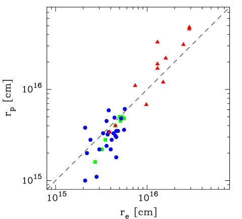
Figure 3: SiO photodissociation radii (obtained using the unshielded photodissociation rate $G_{0}$ = 2.5 $\times$ 10^-10 s^-1) versus the estimated sizes of the SiO envelopes (IRV: square; SRV: circle; Mira: triangle). The dashed line shows the one-to-one relation

6.4 Interferometry data

We have also checked our modelling results by comparing with the interferometric SiO($J$=2$\rightarrow$1) data toward a number of O-rich CSEs of Lucas et al. (1992). They derived the sizes of the SiO line emitting region from direct fits, assuming exponential source-brightness distributions, to the visibility data. Their observations thus yielded the half-intensity angular radii of the SiO($J$=2$\rightarrow$1) emitting regions. Sahai & Bieging (1993) observed a smaller sample of CSEs interferometrically, and claimed that the source brightness distribution is rather of a power-law form (i.e., scale-free). This would explain why Lucas et al. derived essentially the same angular sizes for most of the sources independent of their distances. To resolve this issue requires more detailed observations, and we will only use the results of Lucas et al. to compare with our modelling results.

We have six stars in common with Lucas et al. (1992) (RX Boo, R Cas, W Hya, R Leo, WX Psc, IK Tau). Fig 4 shows the intensity radii as a function of the density measure $\dot{M}/v_{\rm e}$, using our derived mass-loss rates, gas expansion velocities, and distances. The minimum least-square correlation between these intensity radii and the density measure is

$$\log r_{I/2}\,=\,18.8+0.49\,\log\,\left(\frac{\dot{M}}{v_{\rm e}}\right)\,,$$ (14)

(the correlation coefficient is 0.88) where $r_{I/2}$ is given in cm, ${\dot{M}}$ in M_⊙ yr^-1, and $v_{\rm e}$ in km s^-1.

Figure 4: The sizes of the SiO envelopes estimated from the SiO line modelling are plotted versus a density measure (open circles). The dashed line gives the relation between the SiO envelope size and the density measure given in Eq. (13). Half intensity radii derived from interferometric SiO($J$=2$\rightarrow$1) observations are shown as solid circles. The solid line is the fit to the data given in Eq. (14)

Thus, the scaling with the density measure of the intensity radii is in perfect agreement with our modelling result for the envelope sizes. The estimated SiO envelope sizes that are required to model the data are about three times larger than the SiO($J$=2$\rightarrow$1) brightness region. This may at first seem somewhat surprising, but a test using the 10^-6 M_⊙ yr^-1 model star of Sect. 4.4, which has an SiO envelope radius of 1$\aas@@fstack{\prime\prime}$7, shows that the resulting SiO($J$=2$\rightarrow$1) brightness distribution has a half-intensity radius of 0$\aas@@fstack{\prime\prime}$4, i.e., about four times smaller.

7 Results of the SiO line model fits

7.1 The fitting procedure

The radiative transfer analysis produces model brightness distributions. These are convolved with the appropriate beams to allow a direct comparison with the observed velocity-integrated line intensities and to search for the best fit model. As observational constraints we have used the data presented in this paper and the high-frequency data obtained by Bieging et al. (2000). With the assumptions made in the standard circumstellar model and the mass-loss rate and dust properties derived from the modelling of circumstellar CO emission, there remains only one free parameter, the SiO abundance [for all stars $r_{\rm e}$ is taken from Eq. (13)]. The SiO abundance was allowed to vary in steps of $\approx$10% until the best-fit model was found. The quality of a particular model with respect to the observational constraints can be quantified using the chi-square statistic,

$$\chi^{2}_{\rm red}=\frac{1}{\rm N-p}\,\sum^{\rm N}_{i=1}\frac{[I_{\mathrm{mod},i}-I_{\mathrm{obs},i})]^{2}}{\sigma^{2}_{i}},$$ (15)

where $I$ is the total integrated line intensity, $\sigma_{i}$ the uncertainty in observation $i$, p the number of free parameters (2 in the cases of multi-line CO modelling, but only 1 for the SiO line modelling, except in the cases discussed above where also $r_{\rm e}$ was a free parameter), and the summation is done over all independent observations N. The errors in the observed intensities are always larger than the calibration uncertainty of $\approx$20%. We have chosen to adopt $\sigma_{i}$ = 0.2$I_{\mathrm{obs},i}$ to put equal weight on all lines, irrespective of the S/N-ratio. The final chi-square values for stars observed in more than one transition are given in Table 4. They are, in many cases, rather large suggesting that our circumstellar model may not be entirely appropriate for the modelling of the SiO radio line emission, see Sect. 8. The line profiles were not used to discriminate between models, but differences between model and observed line profiles are discussed in Sects 7.4 and 8.

7.2 The accuracy of the estimated abundances

We will here try to estimate the uncertainty in the derived SiO abundances. The uncertainties due to the adopted circumstellar model are ignored since these are very difficult to estimate, and focus is put on those introduced by the adopted parameters (see Sect. 4.4). We start by considering the IRV/SRVs. The results depend crucially on the validity of Eq. (13). A change by $-$50% and +100% in the size of the SiO envelope results in a variation of the $J$=2$\rightarrow$1 line intensity by about $\pm$50%, and therefore an equal uncertainty in the abundance. The product of $f_{\rm SiO}$ and $\dot{M}$ is essentially constant for a best fit model. It is estimated that the mass-loss rate is uncertain by at least a factor of two (due to the modelling). An uncertainty in the distance has only a minor effect on the abundance (the change in mass-loss rate compensates for the change in distance). The dependence on the luminosity is moderate. We therefore estimate that, within the adopted circumstellar model, the derived SiO abundances are uncertain by at least a factor of three for those sources with multi-line observations. The uncertainty increases to a factor of five when only one transition is observed.

For the high mass-loss rate (i.e., $\gtrsim$ 5$\times$10^-6 M_⊙ yr^-1) Miras the situation is even worse. The radiation from these stars are significantly converted into longer-wavelength dust radiation, which has been taken care of only crudely by using two central blackbodies. Tests show that the resulting SiO line intensities are sensitive to the structure of the radiation sources, Sect 4.4. In addition, the SiO lines are rather saturated and hence the line intensities are, at least partly, insensitive to the abundance. Therefore, it is estimated that for these objects the SiO abundance is uncertain by a factor of five (in all cases information on three, or more, lines is available), but note that any reasonable change in the radiation field structure will systematically lower the abundance required to fit the data.

Table 4: Source parameters and SiO model results

Source Var. $$P$$ (SiO) (CO) N

type [days] [pc] [km s^-1] [km s^-1] [10^-7 M_⊙ yr^-1] [10¹⁵ cm] [10¹⁵ cm] [10^-6]

RS And SRa 136 290¹ 14.4 14.4 111.5 12.2 14.0 16.0 1

UX And SRb 400 280¹ 12.8 12.8 114.0 15.9 13.8 12.0 1

Aps SRb 119 110¹ 14.0 14.5 110.4 12.0 12.2 14.0 0.3 3

TZ Aql Lb 470¹ 14.8 14.8 111.0 12.2 13.2 15.0 8.1 2

SV Aqr Lb 470¹ 18.0 18.0 113.0 14.0 14.5 34.0 2.1 2

T Ari SRa 317 310¹ 12.4 12.4 110.4 11.1 12.8 15.2 2.9 2

RX Boo SRb 340 110¹ 17.8 19.3 115.0 14.8 15.2 18.0 1.2 6

RV Cam SRb 101 350¹ 15.8 15.8 112.5 13.0 14.6 14.5 1

TX Cam M 557 380¹ 16.0 18.5 160.0 33.0 13.0 15.5 2.0 3

R Cas M 431 220¹ 17.0 10.5 113.0 11.0 17.4 17.0 0.8 3

UY Cet SRb 440 300¹ 16.0 16.0 112.5 13.1 14.5 16.0 3.0 3

CW Cnc Lb 280¹ 17.0 18.5 115.0 14.5 15.1 12.7 1

R Crt SRb 160 170¹ 10.6 10.6 118.0 16.1 15.7 16.0 2.5 3

R Dor SRb 338 145¹ 15.0 16.0 111.3 13.3 13.3 15.0 2.4 4

AH Dra SRb 158 340¹ 16.4 16.4 110.8 12.0 12.6 17.0 1

CS Dra Lb 370¹ 11.6 11.6 116.0 15.0 15.0 12.7 1

S Dra SRb 136 270¹ 19.6 19.6 114.0 14.9 14.4 17.0 4.3 2

SZ Dra Lb 510¹ 19.6 19.6 116.0 15.0 15.3 11.8 1

TY Dra Lb 430¹ 19.0 19.0 116.0 14.8 15.6 10.0 0.3 2

R Hya M 388 150¹ 14.5 17.0 113.0 14.0 14.5 17.0 4.2 2

W Hya SRa 361 165¹ 16.5 16.5 110.8 12.8 12.4 15.0 4.5 7

R Leo M 313 130¹ 16.0 16.0 112.0 13.9 15.5 13.0 2.5 3

U Men SRa 407 320¹ 17.2 17.2 112.0 13.4 13.8 15.8 3.5 2

T Mic SRb 347 130¹ 14.8 14.8 110.8 12.2 13.0 15.3 1.2 2

GX Mon M 527 540¹ 18.7 18.7 400.0 48.0 29.0 10.8 4.0 5

S Pav SRa 381 150¹ 14.8 19.0 110.8 13.8 12.1 12.6 0.3 2

SV Peg SRb 145 190¹ 16.3 17.5 113.0 13.5 16.5 15.1 1

TW Peg SRb 929 200¹ 19.5 19.5 112.5 14.5 13.6 12.4 1

WX Psc M 660 600¹ 19.3 19.3 110.0 22.0 16.0 16.0 3.1 4

L² Pup SRb 141 185¹ 12.3 12.3 110.2 11.0 12.1 14.0 2.1 3

Y Scl SRb 330¹ 15.2 15.2 111.3 12.4 13.6 15.0 0.7 2

V1943 Sgr Lb 150¹ 14.6 15.4 111.3 12.8 13.5 17.3 1.3 2

IK Tau M 500 250¹ 17.5 18.5 300.0 31.0 25.0 10.4 2.8 4

V Tel SRb 125 290¹ 16.8 16.8 112.0 13.2 13.7 15.0 12.0 2

Y Tel Lb 340¹ 13.5 13.5 115.0 11.6 12.7 54.0 0.1 2

Y UMa SRb 168 220¹ 14.8 14.8 111.5 12.8 14.1 12.0 1

SU Vel SRb 150 250¹ 15.5 15.5 112.0 13.3 14.3 12.7 5.3 2

BK Vir SRb 150 190¹ 14.0 14.0 111.5 11.8 14.6 12.3 1

RT Vir SRb 155 170¹ 16.2 17.8 115.0 13.6 15.6 13.0 1.3 2

SW Vir SRb 150 120¹ 17.5 17.5 114.0 13.5 14.8 13.5 9.1 4

IRC+10365 M 500 750¹ 16.2 16.2 300.0 46.0 29.0 14.0 3.9 3

IRC10529 M 680 270¹ 12.0 12.0 125.0 16.8 10.0 11.1 0.1 3

IRC30398 M 575 390¹ 16.0 16.0 160.0 17.0 13.0 10.3 10.0 3

IRC+40004 M 750 410¹ 18.0 18.0 160.0 19.0 13.0 10.2 8.7 3

IRC+50137 M 629 410¹ 17.0 17.0 100.0 12.0 15.0 10.5 2.0 3

¹ Distance derived assuming a luminosity of 4000 L_⊙

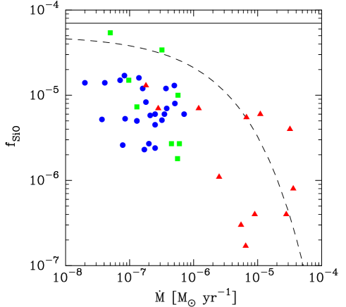
Figure 5: SiO fractional abundances versus the mass-loss rate (IRV:square, SRV:circle, Mira:triangle). The horizontal line marks the maximum abundance allowed by solar abundances. The dashed line shows the expected $f(\infty)$ (scaled to 5$\times$10^-5, roughly the expected abundance from stellar equilibrium chemistry, at very low mass-loss rates) for the parameters given in Sect. 8

7.3 Abundances

It can be assumed that the stars in our samples have silicon abundances close to the solar value, Si/H = 3.6$\times$10^-5 (Anders & Grevesse, 1989). If Si is fully associated with O as SiO, and all H is in H₂, the maximum SiO fractional abundance is 7$\times$10^-5. Detailed calculations on stellar atmosphere equilibrium chemistry give abundances in the vicinity of this for M-stars, about 4$\times$10^-5 (Duari et al., 1999). Duari et al. also show that the SiO abundance is not affected by atmospheric shocks in the case of M-stars.

The derived SiO abundances are given in Table 4. The distribution for the IRV/SRV sample has a median value of 6$\times$10^-6, and a minimum of 2$\times$10^-6 and a maximum of 5$\times$10^-5. For the IRVs and SRVs the median results are 9$\times$10^-6 and 6$\times$10^-6, respectively. This is almost a factor of ten lower than expected from theory. Figure 5 shows the SiO abundance as a function of the mass-loss rate. In addition to the abundances being low, there is also a trend in the sense that both the upper and the lower ‘envelope’ of the abundances decrease with increasing mass-loss rate.

Figure 6: Comparison of observed CO (upper) and SiO (lower) line profiles (in histogram form) for R~Dor (left) and R~Hya (middle) and GX~Mon (right). The corresponding best-fit (i.e., to all observed line intensities) model SiO lines are also shown as solid lines

The low mass-loss rate Miras follow the trend of the IRV/SRVs, and for the high mass-loss rate ($\dot{M}>5\times 10^{-6}$ M_⊙ yr^-1) Miras we find a substantially lower abundance, a median below 10^-6. Thus, the inclusion of the Miras shows that the trend of decreasing SiO abundance with increasing mass-loss rate continues towards high mass-loss rates. This is further discussed in Sect. 8 where an interpretation in terms of increased adsorption of SiO onto dust grains the higher the mass-loss rate is advocated.

The spread in abundance, at a given mass-loss rate, is substantial, but it is within the (considerable) uncertainties, except possibly for the high mass-loss rate Miras, for which there seem to be a division into a low abundance group (on average 4$\times$10^-7) and a high abundance group (on average 5$\times$10^-6), while . This division into two well-separated groups is peculiar, but within the circumstellar model used here this conclusion appears inescapable. One can argue that the modelling of the high mass-loss rate Mira SiO line emission is particularly difficult, but we find no reason why errors in the model should affect stars with essentially similar properties ($L$, $\dot{M}$, $v_{\rm e}$) so differently.

7.4 CSE dynamics

The observed SiO line profiles are used in the modelling to derive the gas expansion velocities in the regions of the CSEs where the observed SiO line emission stems from. A comparison of these values with the gas expansion velocities derived from the modelling of circumstellar CO line emission is indeed a direct probe of the CSE dynamics since the extents of the SiO and CO line emitting regions are very different.

The SiO and CO radio line profiles are clearly different, although this conclusion is mainly based on the limited number of sources where the S/N-ratio of the data are high enough for both species. In Table 4 different values for the gas expansion velocity estimated from the SiO and the CO data are reported in the 11 cases where these are regarded as significantly different. In all cases the SiO velocities are smaller than those obtained from the CO data. Indeed, the SiO line profiles are narrower in the sense that the main fraction of the emission comes from a velocity range narrower than twice the expansion velocity determined from the CO data. On the other hand, the SiO line profiles have weak wings so that the total velocity width of its emission is very similar to that of the CO emission. This is illustrated in Fig. 6, where we also show the corresponding best-fit (i.e., to all observed line intensities) model SiO lines. It is clear that the model line profiles do not provide perfect fits to the observed line profiles, but they show that for the lower mass-loss rate objects the SiO line profiles are strongly affected by selfabsorption on the blue-shifted side. This explain partly why the SiO lines are narrower than the CO lines. The remaining discrepancy is interpreted as due to the influence of gas acceleration in the region which produces a significant fraction of the SiO line emission, as suggested already by Bujarrabal et al. (1986). This interpretation is quantitatively corroborated by our modelling results when a velocity gradient is included, see Sect. 4.4. The extent of the effect is though uncertain. Bieging et al. (2000), by comparing high-$J$ SiO lines with CO line data, concluded that the SiO lines are formed predominantly in the part of the CSE where the gas velocity exceeds 90% of the terminal velocity. We suspect that the discrepancy between the widths of the SiO and CO lines decreases with the mass-loss rate of the object. In addition, we find that for at least some of the high-mass-loss-rate sources the higher-$J$ SiO lines become essentially triangular, see GX~Mon in Fig. 6. The model does a fairly good job in reproducing these SiO line profiles, except that the model lines are less sharply peaked. A high sensitivity, multi-line study combined with interferometric observations are required to fully tackle this problem.

In this connection we also present Fig. 7 which shows the gas expansion velocity (determined from CO line modelling) as a function of mass loss rate for the IRV/SRV and Mira samples. This is an extension of the result of Olofsson et al. (2002), and it shows that low to intermediate mass-loss rate winds have a scaling of $v_{\rm e}\propto\dot{M}^{0.36}$, and that this gradually goes over into a wind of close to 20 km s^-1, for higher mass-loss rates. This is as expected for a dust-driven wind (Elitzur & Ivezić, 2001).

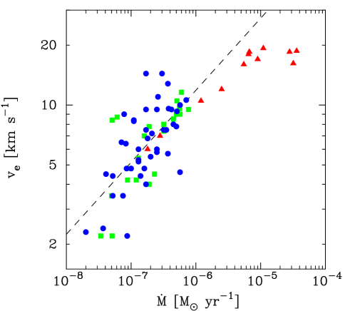
Figure 7: The derived CO gas expansion velocities as a function of the mass-loss rates for the IRV (squares), SRV (circles), and Mira (triangles) samples. The dashed line shows the correlation found for the IRV/SRV sample (see text)

7.5 Peculiar sources

To single out peculiar sources is a highly subjective process, and it also depends strongly on the S/N-ratio of the data (at high enough S/N-ratio probably most sources show a deviation from the expected). Here, a few sources in the IRV/SRV sample which qualify as peculiar or for which we have problems in the SiO line modelling are discussed.

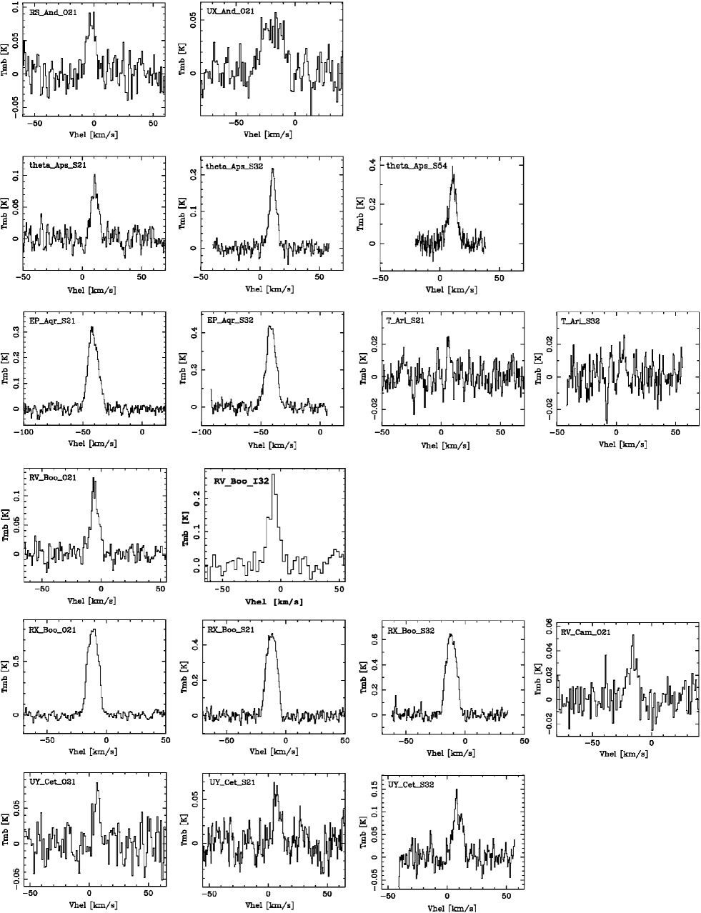
Figure 10: SiO spectra of M-type SRVs (Part 1). Note the heliocentric velocity scale

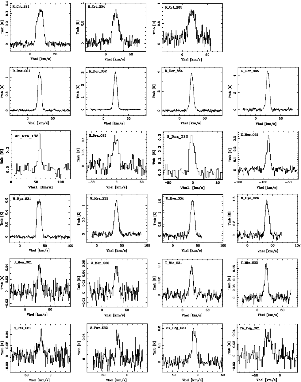
Figure 11: SiO spectra of M-type SRVs (Part 2). Note the heliocentric velocity scale

Kerschbaum & Olofsson (1999) found four objects in their sample of circumstellar CO radio line emission, which clearly show double-component line profiles, a narrow feature centred on a broad plateau (EP~Aqr, RV~Boo, X~Her, and SV~Psc), all of them SRVs. Olofsson et al. (2002) determined mass-loss rates and gas expansion velocities by simply decomposing the emission into two components and assuming that the emissions are additive. They found that the mass loss rates are higher for the broader component by, on average, an order of magnitude. The gas expansion velocities derived from the narrow components ($\approx$1.5 km s^-1) put to question an interpretation in the form of a spherical outflow. The origin of such a line profile is still not clear (see Olofsson et al. (2002) for a discussion on this issue). These four sources are also included in our SiO sample, and the spectra are shown in Figs. 10 and 11.

Towards EP~Aqr there is no sign of the narrow feature in the SiO $J$=2$\rightarrow$1 and $J$=3$\rightarrow$2 lines, only the broad feature is clearly present. This suggests that the broad feature originates in a ‘normal’ CSE, while the narrow feature may have a different origin. We note though that the SiO line profile of the broad component deviates somewhat from a smooth symmetric profile. SV~Psc is very similar to EP~Aqr in CO in the sense that the narrow feature is very much narrower than the broad feature. Unfortunately, the SV~Psc SiO data are of low quality, but both components appear to be present. In the cases of RV~Boo and X~Her the CO and SiO line profiles are very similar, and the widths of the narrow components are about half of those of the broad ones. The SiO abundances of both components have been obtained, assuming that the emissions are additive. The results are given in Table 5. For all sources, and for both components, the results appear normal.

Figure 8: L$^2$~Pup SiO line spectra and a CO($J$=3$\rightarrow$2) spectrum (from Olofsson et al. (2002))

Table 5: Source parameters and model results for those objects with double component line profiles

Source Var. $$P$$00 comp. (SiO) (CO) N

type [days] [pc] [10^-7 M_⊙ yr^-1] [km s^-1] [km s^-1] [10¹⁵ cm] [10^-6]

EP Aqr SRb 155 140 broad 5.0 7.8 9.2 5.2 13.8 2

RV Boo SRb 137 280 broad 2.0 6.8 7.0 3.2 16.0 2

narrow 0.3 3.0 2.3 2.6 17.0 1

X Her SRb 195 140 broad 1.5 6.5 6.5 3.4 12.0 1

narrow 0.4 2.5 2.2 3.1 14.0 1

SV Psc SRb 102 380 broad 3.0 8.6 9.5 4.0 10.0 3

narrow 0.4 1.6 2.2 3.2 16.0 1

L$^2$~Pup was singled out in Olofsson et al. (2002) as a low mass-loss rate (2$\times$10^-8 M_⊙ yr^-1), low gas expansion velocity (2.1 km s^-1) object. This star has been recently discussed also by Jura et al. (2002) and Winters et al. (2002). In the latter paper comparisons are made with wind models, and it is concluded that stars with the mass-loss properties of L$^2$~Pup can be understood in terms of a pulsationally driven wind, where dust plays no dynamic role. Our SiO line profiles resemble to some extent those of CO in the sense that the narrow feature is also present. However, the SiO lines clearly show broad line wings, Fig. 8. The full velocity width of these lines are $\approx$ 12 km s^-1, i.e., larger than the CO line width, but narrower than the SiO($v$=1, $J$=2$\rightarrow$1) maser line width of $\approx$ 20 km s^-1 measured by Winters et al. (2002). In addition, the narrow feature, which appears narrower in the SiO lines than in the CO lines (Fig. 8), is not exactly centered on the broad component, its center lies at $v_{\rm hel}$ = 52.8 km s^-1 as opposed to 51.4 km s^-1 for the latter. This suggests a rather complicated dynamics in the inner part of the CSE, but high-quality data, also in higher-$J$ SiO lines, are required before progress can be made.

W~Hya is one of the sources for which we have the highest quality data. It is also one of the sources with the poorest best-fit model. A much better fit is obtained by increasing the size of the SiO envelope to $r_{\rm e}$=6$\times$10¹⁵ cm (and $f_{\rm SiO}$=8$\times$10^-6 as determined from the high-$J$ lines), i.e., almost a factor of three higher than that obtained from Eq.(13). Considering the uncertainties this is of no major concern. However, it is worth recalling that Olofsson et al. (2002) derived a (molecular hydrogen) mass-loss rate of 7$\times$10^-8 M_⊙ yr^-1 from CO data [this result has been confirmed by including CO $J$=1$\rightarrow$0 and 2$\rightarrow$1 IRAM 30 m data (Bujarrabal et al., 1989; Cernicharo et al., 1997), CO $J$=2$\rightarrow$1, 3$\rightarrow$2, and 4$\rightarrow$3 JCMT archive data, and the CO ISO results of Barlow et al. (1996)], while Zubko & Elitzur (2000) required a much higher mass-loss rate, 2.3$\times$10^-6 M_⊙ yr^-1 (at the larger distance 115 pc) to explain the ISO H₂O data. We have found that such a high mass-loss rate produces CO radio lines that are at least a factor of 30 too strong. However, the ISO CO $J$=16$\rightarrow$15 and $J$=17$\rightarrow$16 lines are only about a factor of two too strong. Hence, there is some considerable uncertainty in the properties of this CSE. A fit to the SiO line data using the larger distance and mass-loss rate is as bad as that for the low distance and mass-loss rate.

In the case of R~Dor Olofsson et al. (2002) could not fit well the CO radio line profiles. The model profiles were sharply double-peaked, while the observed ones were smoothly rounded. We merely note here that there was no problem to fit the SiO line profiles with the nominal values for R~Dor.

8 Discussion and conclusions

An extensive radiative transfer analysis of circumstellar SiO ‘thermal’ radio line emission from a large sample of M-type AGB variable stars have been performed, partly based on a new, large, observational data base. It is concluded that, at this stage, the modelling of the circumstellar SiO radio line emission is considerably more uncertain than that of the CO radio line emission. Partly because the SiO line emission predominantly comes from the inner regions where the observational constraints are poor, but also partly because the behaviour of the SiO molecule is more complex, e.g., adsorption onto grains. A rather detailed sensitivity analysis has been done, in order to estimate the reliability of the derived results.

In particular, the size of the SiO envelope is crucial to the modelling. Multi-line SiO modelling of eleven sources were used to establish a relation between the size of the SiO envelope and the density measure $\dot{M}/v_{\rm e}$. This is of course rather uncertain, both in the absolute scale and in the dependence on the density measure. Comparison with estimates based on rather simple condensation and photodissociation theories suggests that the derived relation is not unreasonable. A very good agreement with the photodissociation radii is obtained for an unshilded photodissociation rate of 2.5 $\times$ 10^-10 s^-1. It was also checked against interferometeric SiO line brightness size estimates of six sources.

The SiO abundance distribution of the IRV/SRV sample has a median value of 6$\times$10^-6, and a minimum of 2$\times$10^-6 and a maximum of 5$\times$10^-5. For these, low to intermediate mass-loss rate objects, we expect the abundances to be representative for the region inside the SiO photodissociation radius. This applies also to the low and intermediate mass-loss rate Miras. The high mass-loss rate Miras have a median abundance which is more than a factor of six lower than that of the IRV/SRV sample. The derived SiO abundances are in all cases (within the uncertainties) below the abundance expected from stellar atmosphere chemistry ($\approx$ 4$\times$10^-5, Duari et al. (1999)), the median for the total sample is down by a factor of ten. We regard this as a safe result, and interpret it in terms of SiO adsorption onto grains, which is efficient already at low mass-loss rates.

In addition, there is a trend of decrasing SiO abundance with increasing mass-loss rate, Fig. 5. Here, we cannot entirely exclude systematic effects of the modelling. In particular, the adopted SiO envelope size relation can introduce such effects. E.g., smaller envelopes at low mass-loss rates, as indicated by the photodissociation model, would increase the estimated abundances for these objects. This will actually strenghten the observed trend. There is no obvious reason for a similar envelope size decrease for the high mass-loss rate objects (however, see below), but if present it would lead to a less pronounced trend. The discussion in Sect. 4.4 on the sensitivity on the radiation field distribution suggests that the abundance estimates for the high mass-loss rate objects are upper limits. Therefore, considering also that the effect is rather large, we regard the trend as at least tentative. An interpretation in terms of increased adsorption of SiO onto grains with increasing mass-loss rate is natural. In Fig. 5 a depletion curve based on the results in Sect. 6.1 is plotted, and it represents well the general trend (the adopted parameters are $T_{\rm bb}$ = 2500 K, $L$ = 4000 L_⊙, $v_{\rm e}$ = 10 km s^-1, $\psi$ = 0.002, $a_{\rm gr}$ = 0.05 $\mu$m, $\rho_{\rm gr}$ = 2 g cm^-3, $Q_{\rm p,F}$ = 0.03, $T_{\rm bind,SiO}$ = 29500 K, and $\alpha$ = 1). We emphasize once again how sensitive the theoretical condensation results are to the adopted parameters, and the depletion curve can easily be made to fit better the estimated abundances.

For the high mass-loss rate Miras the SiO abundance distribution appears bimodal, a low abundance group (on average 4$\times$10^-7) and a high abundance group (on average 5$\times$10^-6). At this point we cannot identify any reason for this. The stars and their CSEs are rather similar and there is no reason to expect the modelling to artificially produce very different results for rather similar objects, but the SiO line modelling of these objects are particularly difficult as discussed above. The high values can be explained if there is a process which decreases the condensation onto, or leads to effective evaporation from, dust grains for some objects. The former is possible if the dust-to-gas mass ratio is low. If, on the other hand, the dust-to-gas mass ratio is high, the region contributing to the SiO line emission may be much smaller than used in our modelling, and hence the SiO abundance is underestimated. This may be the case for the low abundance objects. Substantial mass-loss rate variations with time may of course lead to surprising results. This can possibly be checked by high angular resolution observations of both CO and SiO radio line emission. It is also interesting that Woods et al. (2003) found, in a sample of high mass-loss rate C-stars, that the SiO abundance is one of the few of their abundance estimates that vary significantly from star to star. We note, though, that for the C-stars the estimated SiO abundances are low, about 1$\times$10^-7, and that Willacy & Cherchneff (1998) have shown that for C-stars shock chemistry may significantly alter the SiO abundance. The same is not the case for the O-rich chemistry according to Duari et al. (1999), but grains are not included in their analysis.

The SiO and CO radio line profiles differ in shape. For those stars with high enough S/N-ratio data on both species, it is clear that the dominating parts of the SiO profiles are narrower than the CO profiles, but the former have low-intensity wings which cover the full velocity range of the CO profile. The effect is more evident in high-$J$ lines, and less evident in high mass-loss rate objects. This is interpreted (as has been done also by others) as due to the influence of gas acceleration in the region which produces most of the SiO line emission. This points to a weakness in our analysis. Clearly, this acceleration region must be treated more carefully in the radiative modelling, but this is also the region where condensation occurs, a process which is difficult to describe in detail.

These results strongly suggest that SiO radio line emission can be used as a sensitive probe of circumstellar dust formation and dynamics. However, considerable progress in this area can only be expected from a combination of high-quality SiO multi-line observations, high-quality interferometric observations of a number of SiO lines for a representative sample of sources, a detailed radiative transfer analysis, which includes also the dust radiation, and a detailed SiO chemical model. The rather high $\chi^{2}$ values of some of our best-fit models suggest that our circumstellar model needs to be improved.

Olofsson et al. (2002) identified a number of sources with peculiar CO line profiles, essentially consisting of a narrow feature centered on a (much) broader feature. These have been discussed here from the point of view of their SiO line properties. Except in one case, the SiO and CO line profiles are rather similar, and the derived SiO abundances are in no case peculiar. The low gas expansion velocity source L² Pup has a very narrow SiO line profile as expected, but also a considerably broader, low-intensity component. Finally, W Hya imposes a problem for the SiO line modelling. In principle, a much larger SiO envelope than warranted by the mass-loss rate derived from the CO data is required to fit well the (high-quality) SiO data. This, in combination with other data, suggest that the CSE of this star is not normal, possibly as an effect of time-variable mass loss.

Appendix A Observational results

Table 6: Observational results of circumstellar SiO radio line emission towards a sample of M-type IRVs and SRVs (Part 1)

GCVS4 IRAS Code S $$I$$ 00 00 00 Q C

[K km s^-1] [K] [km s^-1] [km s^-1] [km s^-1]

BC And 22586+4614 O21 N 110.2 5

RS And 23528+4821 O21 D 110.71 0.076 3.1 4.2 6.1 3

UX And 02302+4525 O21 D 110.94 0.044 19.4 20.1 16.6 3

Aps 14003–7633 S21 D 110.62 0.078 10.8 3.1 6.1 2

S32 D 111.4 0.18 10.9 3.2 5.6 2

S54 D 112.7 0.30 10.7 3.0 7.6 2

TZ Aql 20276–0455 S21 D 110.15 0.025 49.3 62.3 5.0 3

S32 D 110.14 0.026 49.4 62.4 4.5 4

V584 Aql 20079–0146 S21 N 110.2 5

S32 N 110.1 5

AB Aqr 22359–1417 S21 N 110.1 5

S32 N 110.1 5

EP Aqr 21439–0226 S21 D 113.2 0.28 41.3 31.9 8.2 2

S32 D 114.4 0.40 41.3 31.9 7.9 2

SV Aqr 23201–1105 S21 D 110.54 0.036 7.3 8.5 9.5 3

S32 D 110.66 0.070 6.6 7.8 7.2 2

T Ari 02455+1718 O21 D 110.084 0.043 6.5 1.2 1.5 4

S21 D 110.081 0.021 6.4 1.4 2.9 4

S32 D 110.091 0.017 5.5 2.2 4.0 4

RV Boo 14371+3245 O21 D 110.79 0.069 5.0 9.5 6.5 b

O21 D 110.19 0.051 6.0 8.5 2.0 n

O21 D 110.98 0.12 6.9 7.6 8.8 2 b+n

I32 D 112.5 0.25 5.9 8.6 8.0 b+n

RX Boo 14219+2555 O21 D 119.5 0.84 12.1 0.2 9.0 1

S21 D 115.1 0.44 11.6 0.7 8.7 1

S32 D 116.4 0.61 11.7 0.6 8.2 1

RV Cam 04265+5718 O21 D 110.32 0.036 15.9 16.0 6.8 4

BI Car 10416–6313 S21 N 110.2 5

S32 N 110.3 5

SS Cep 03415+8010 O21 N 110.3 5

V744 Cen 13368–4941 S21 N 110.1 5

S32 N 110.4 5

V806 Cen 13465–3412 S21 N 110.3 5

S32 N 110.2 5

UY Cet 00245–0652 O21 D 110.41 0.071 6.5 3.6 4.6 4

S21 D 110.38 0.053 7.8 4.9 5.2 4

S32 D 111.02 0.11 8.9 6.0 7.1 3

CW Cnc 09057+1325 O21 D 110.62 0.065 26.6 17.2 7.9 3

R Crt 10580–1803 S21 D 115.0 0.33 19.6 11.9 10.9 1

S54 D 119.9 0.66 19.8 12.1 10.7 2

S65 D 113.6 0.86 19.0 11.3 12.6 3

V CVn 13172+4547 O21 N 110.3 5

W Cyg 21341+4508 O21 N 110.1 5

U Del 20431+1754 O21 N 110.5 5

R Dor 04361–6210 S21 D 119.6 1.1 23.9 7.5 6.1 1

S32 D 124.0 2.8 24.0 7.6 6.0 1

S54 D 131.1 3.6 24.4 8.0 6.0 1

S65 D 134.7 5.1 24.4 8.0 5.8 1

AH Dra 16473+5753 I32 D 111.2 0.17 57.6 74.9 8.5

CS Dra 11125+7524 O21 D 110.41 0.022 60.1 51.3 12.5 4

S Dra 16418+5459 O21 D 111.4 0.10 2.2 15.4 9.9 4

I32 D 113.6 0.30 1.6 15.9 8.6 3

SZ Dra 19089+6601 O21 D 110.17 0.024 44.2 28.3 4.8 4

TY Dra 17361+5746 O21 D 110.65 0.038 33.9 18.9 11.5 4

I32 D 113.2 0.22 34.0 16.4 11.1 3

UU Dra 20248+7505 O21 N 110.3 5

g Her 16269+4159 O21 N 110.2 5

X Her 16011+4722 O21 D 112.2 0.18 90.5 73.0 8.0 b

O21 D 110.53 0.16 89.5 72.0 2.2 n

O21 D 112.7 0.34 90.7 73.2 7.4 1 b+n

FZ Hya 08189+0507 O21 N 110.7 5

Table 7: Observational results of circumstellar SiO radio line emission towards a sample of M-type IRVs and SRVs (Part 2)

GCVS4 IRAS Code S $$I$$ 00 00 00 Q C

[K km s^-1] [K] [km s^-1] [km s^-1] [km s^-1]

W Hya 13462–2807 S21 D 116.0 0.63 38.5 40.4 7.1 1

S32 D 110.9 1.2 39.2 41.1 6.4 1

S54 D 113.2 0.98 39.2 41.1 7.1 1

S65 D 113.2 0.86 39.4 41.3 6.7 1

RW Lep 05365–1404 S21 N 110.3 5

S32 N 110.1 5

U Men 04140–8158 S21 D 110.30 0.037 28.9 17.0 6.3 3

S32 D 110.44 0.049 28.7 16.8 6.5 3

T Mic 20248–2825 S21 D 110.67 0.088 17.7 25.3 5.6 2

S32 D 111.2 0.16 17.8 25.4 5.6 2

EX Ori 05220–0611 O21 N 110.7 5

V352 Ori 05592–0221 O21 N 110.5 5

S Pav 19510–5919 S21 D 110.32 0.030 19.2 20.0 8.3 3

S32 D 110.40 0.055 19.1 19.9 5.6 4

NU Pav 19575–5930 S21 N 110.1 5

S32 N 110.3 5

SV Peg 22035+3506 O21 D 112.1 0.18 8.3 2.1 9.5 2

TW Peg 22017+2806 O21 D 110.54 0.035 23.0 10.5 9.3 4

SV Psc 01438+1850 O21 D 110.45 0.05 9.5 5.7 6.9 3 b+n

S21 D 110.31 0.03 10.5 6.7 11.0 3 b+n

S54 D 110.63 0.06 10.4 6.6 8.4 3 b

S54 D 110.20 0.10 10.4 6.6 1.6 3 n

S54 D 110.83 0.10 10.2 6.4 6.3 3 b+n

V PsA 22525–2952 S21 N 110.1 5

S32 N 110.1 5

L² Pup 07120–4433 S21 D 110.83 0.14 52.4 33.6 4.6 2

S32 D 111.7 0.30 52.0 33.3 3.5 2

S54 D 112.5 0.54 52.3 33.6 3.6 1

Y Scl 23063–3024 S21 D 110.22 0.024 30.9 29.5 6.4 4

S32 D 110.28 0.036 31.8 30.4 5.8 3

CZ Ser 18347–0241 O21 N 110.4 5

Ser 15341+1515 O21 N 110.2 5

S21 N 110.2 5

S32 N 110.1 5

SU Sgr 19007–2247 S21 N 110.1 5

S32 N 110.2 5

V1943 Sgr 20038–2722 S21 D 110.96 0.13 23.1 14.4 5.4 2

S32 D 111.7 0.26 23.0 14.3 4.8 2

V Tel 19143–5032 S21 D 110.59 0.063 34.6 31.8 7.1 3

S32 D 110.40 0.060 35.0 32.2 5.4 3

Y Tel 20165–5051 S21 D 110.21 0.034 46.7 45.3 3.8 4

S32 D 110.44 0.066 45.8 44.4 4.6 3

AZ UMa 11445+4344 O21 N 110.2 5

Y UMa 12380+5607 O21 D 111.2 0.14 8.8 18.6 6.0 2

SU Vel 09480–4147 S21 D 110.35 0.035 20.8 7.0 7.4 3

S32 D 110.38 0.041 20.8 7.0 7.4 3

BK Vir 12277+0441 O21 D 110.63 0.10 15.1 17.8 4.7 3

RT Vir 13001+0527 O21 D 113.8 0.39 13.5 18.7 7.4 2

S21 D 113.2 0.27 13.4 18.6 9.2 2

RW Vir 12046–0629 O21 N 110.4 5

SW Vir 13114–0232 O21 D 113.5 0.33 14.5 9.8 7.9 2

Table 8: Observational results of circumstellar CO and SiO line emission towards our Mira sample

GCVS4 IRAS Molecule Code $$I$$

[K km s^-1] [K] [km s^-1] [km s^-1]

TX Cam 04566+5606 CO O10 121.5 0.88 11.5 20.0

I10 167.0 1.44 11.5 21.0

I21 241.3 3.93 11.4 20.7

J21 169.7 2.61 11.4 20.2

J32 167.2 6.14 11.3 20.3

SiO O21 113.2 0.52 10.7 18.6

R Cas 23558+5106 CO O10 118.4 0.46 24.9 12.2

J21 132.1 1.78 24.8 11.1

J32 100.2 5.48 25.2 11.0

J43 189.6 5.44 24.8 11.9

SiO O21 118.6 0.67 26.3 9.4

R Hya 13269–2301 CO S10 110.6 0.09: -9.7: 5.3:

J32 143.0 3.65 10.5 8.6

SiO S21 112.8 0.44 11.5 5.2

S54 117.7 1.30 11.2 5.9

R Leo 09448+1139 CO O10 112.4 0.25 0.2 7.4

J21 115.0 1.30 0.4 8.7

J32 141.6 3.88 0.3 7.8

SiO O21 115.1 0.51 0.5 6.8

S21 114.9 0.65 0.2 6.9

S54 110.8 1.58 0.4 6.3

GX Mon 06500+0829 CO O10 149.6 1.55 9.3 24.4

J21 167.2 2.27 9.5 18.2

J32 187.6 2.96 9.4 17.9

J43 156.2 1.82 8.7 17.5

SiO O21 119.4 0.36 9.6 19.5

S21 115.5 0.29 9.6 18.9

S54 118.9 0.42 9.1 18.7

WX Psc 01037+1219 CO O10 152.0 1.61 9.6 18.6

J21 131.0 1.31 10.1 18.3

J32 145.5 1.63 9.5 20.8

J43 149.9 1.82 9.5 20.6

SiO O21 110.0 0.40 10.1 18.9

S21 115.6 0.22 9.3 19.2

S54 116.8 0.29 9.3 17.7

IK Tau 03507+1115 CO O10 158.6 1.70 34.4 17.2

J21 103.8 3.32 34.5 17.5

J32 143.8 4.81 34.2 17.6

J43 127.0 4.52 33.2 18.0

SiO O21 116.1 0.66 33.9 18.1

S54 118.9 0.73 34.7 17.5

S65 113.7 0.61 34.7 15.9

IRC+10365 18349+1023 CO O10 121.5 0.79 31.3 16.9

J21 142.0 1.48 30.7 15.3

SiO O21 116.3 0.30 32.6 15.6

IRC–10529 20077–0625 CO O10 115.7 0.65 18.1 15.7

J21 124.4 1.18 17.5 17.7

J32 148.0 2.22 17.1 14.2

J43 157.4 2.87 17.2 16.0

SiO O21 112.9 0.16 17.7 14.6

IRC–30398 18560–2954 CO J21 144.6 1.76 6.4 19.4

SiO S21 110.8 0.06: 10.1: 15.3:

IRC+40004 00042+4248 CO O10 124.8 0.82 20.5 19.2

J21 141.5 1.41 20.5 18.9

SiO O21 111.3 0.05 21.3 20.3

IRC+50137 05073+5248 CO J21 136.8 1.40 3.5 18.7

J32 135.7 1.32 3.3 18.1

SiO O21 112.0 0.10 1.4 14.4

Appendix B Spectra

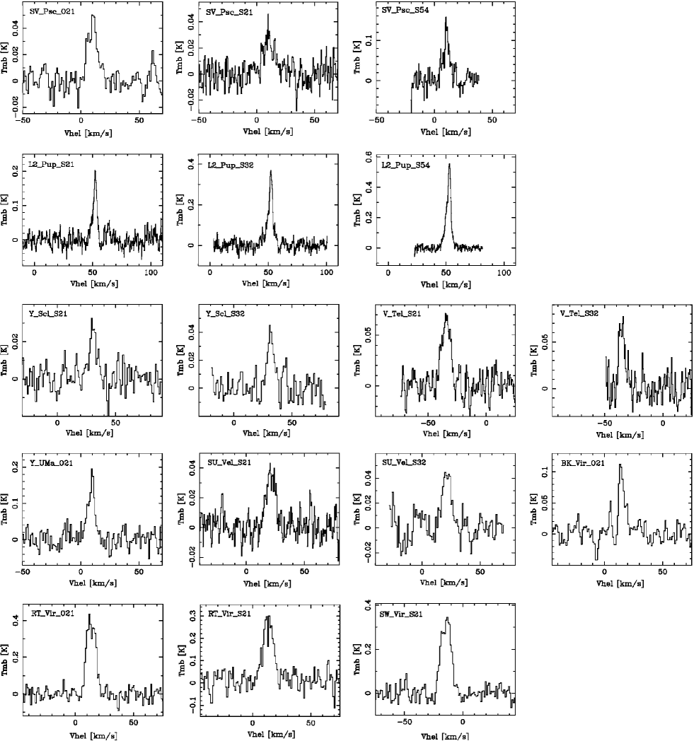
Figure 12: SiO spectra of M-type SRVs (Part 3). Note the heliocentric velocity scale