Precision Cosmology from the Lyman-$\alpha$ Forest: Power Spectrum and Bispectrum

Abstract

We investigate the promise of the Ly-$\alpha$ forest for high precision cosmology in the era of the Sloan Digital Sky Survey using low order N-point statistics. We show that with the existing data one can determine the amplitude, slope and curvature of the slope of the matter power spectrum with a few percent precision. Higher order statistics such as the bispectrum provide independent information that can confirm and improve upon the statistical precision from the power spectrum alone. The achievable precision is comparable to that from the cosmic microwave background with upcoming satellites, and complements it by measuring the power spectrum amplitude and shape at smaller scales. Since the data cover the redshift range $2<z<4$, one can also extract the evolution of the growth factor and Hubble parameter over this range, and provide useful constraints on the presence of dark energy at $z>2$.

1 Introduction

The study of the Ly-$\alpha$ forest has been revolutionized in recent years by high resolution measurements using the Keck HIRES spectrograph (Vogt et al., 1994) and by the development of theoretical understanding using hydrodynamical simulations (Cen et al., 1994; Zhang et al., 1995; Hernquist et al., 1996; Theuns et al., 1998) and analytical models (Gnedin & Hui, 1998). The picture that has emerged from these studies is one in which the neutral gas responsible for the absorption is in a relatively low density, smooth environment, which implies a simple connection between the gas and the underlying dark matter. The neutral fraction of the gas is determined by the interplay between the recombination rate (which depends on the temperature of the gas) and ionization caused by ultraviolet photons. Photoionization heating and expansion cooling cause the gas density and temperature to be tightly related, except where mild shocks heat up the gas. This leads to a tight relation between the absorption and the gas density. Finally, the gas density is closely related to the dark matter density on large scales, while on small scales the effects of thermal broadening and Jeans smoothing have to be included. In the simplest picture described here all of the physics ingredients are known and can be modeled.

Within the model described above, the relation between the observed flux and the underlying dark matter is completely defined, enabling one to study the dark matter correlations with the help of the Lyman-$\alpha$ forest. This was proposed first by Croft et al. (1998) and has been subsequently investigated and applied to the real data by several groups (Croft et al., 1999, 2002b; McDonald et al., 2000; Hui et al., 2001). This work established the simple flux power spectrum as the statistic of choice, although other statistics such as the flux probability distribution have also been investigated (McDonald et al., 2000).

This paper addresses in more detail the question of how much information about cosmological parameters can be extracted from the analysis of the Lyman-$\alpha$ forest and what are the best statistics to use. We focus on N-point statistics (where N=2, 3, 4), since these provide the simplest parametrization of the long-range correlations. We use a Fisher matrix analysis to assess the uncertainties in cosmological parameters for a given uncertainty in Lya forest measurements. To calculate the Fisher matrix, we must calculate the derivatives of the observables (flux power spectrum and bispectrum) with respect to cosmological parameters, centered on a reasonable fiducial model. Using this approach, we show that higher order statistics add to and independently confirm the information gained from the flux power spectrum, and we address practical issues of such a study. For the data sample, we assume a sample with noise and resolution characteristics of the Sloan Digital Sky Survey, which currently contains a few thousand QSO spectra with measured Lyman-$\alpha$ forest ($z>2.2$).

Statistical correlations in the Lyman-$\alpha$ forest are sensitive to several parameters of cosmological interest. Broadly, they are sensitive to the linear power spectrum of matter fluctuations on scales around 1 comoving $h^{-1}$Mpc. In this paper, this power spectrum $P_{L}(k,a)$ is expressed as

$$P_{L}(k,a)=AD^{2}(a)k^{n+(\alpha/2)\ln{(k/k_{p})}}T^{2}(k).$$ (1)

The parameters that are being studied are the power spectrum amplitude ($\kappa\equiv\ln{\sqrt{A}}$), the primordial slope $n$, and primordial curvature $\alpha$. We also investigate the sensitivity to the linear growth factor $D(a)$, where $a=(1+z)^{-1}$ is the expansion factor.

Several additional parameters affecting absorption in the Lyman-$\alpha$ forest must be included, such as those of the gas temperature-density relation, which for our redshift range is assumed to have the form

$$T(\rho)=T_{1.4}\left(\frac{\rho}{1.4\bar{\rho}}\right)^{\gamma-1}.$$ (2)

$T_{1.4}$ is used because McDonald et al. (2001) determined the temperature at this density most precisely. $T_{1.4}$ and $\gamma$ are two of the parameters studied in this paper. In addition, the mean transmitted flux $\bar{F}(z)$ is also assumed to be a free parameter (which can be related to the UV background and baryon density though the equation of ionizing equilibrium). Thus six parameters were varied at each redshift. Our approach is to use hydrodynamical and N-body simulations, and vary all the parameters at each redshift. We are interested in the sensitivity to cosmological parameters, so we marginalize over all the other parameters when presenting the results.

The outline of the paper is the following. In section 2 we describe our HPM simulations and the hydrodynamic simulations that are used for comparison, introduce the statistics used in the course of the analysis, and discuss our choice of simulations, filters and instrumental effects for this study. Section 3 describes the procedure of calculating the Fisher matrix, and the determination of errorbars for the parameters of interest. In section 4, we address the possibility of using the Lyman-$\alpha$ forest to determine quintessence density $\Omega_{q}$ or equation of state $w_{q}$, and more general deviations from the Einstein-de Sitter growth factor $D(a)=a$. After discussing the implications of the results in section 5, we conclude with a discussion of future work in this area.

2 Simulations

To assess the sensitivity of the Ly-$\alpha$ forest to cosmological parameters we performed a Fisher matrix analysis (e.g. Tegmark et al. (1997)). We conducted a redshift-dependent analysis using 9 redshift bins, centered at $z=2.2,2.4,\ldots,3.8$ and using a realistic redshift distribution of quasars as found in SDSS data. Since we only had simulations with values of $a$ spaced by 0.04, we chose the closest $a$ available.

We use Hydro-PM (HPM) simulations (Gnedin & Hui, 1998; McDonald, 2001; McDonald et al., 2002; Cen & McDonald, 2002) rather than more accurate hydrodynamic simulations due to the very large number of simulations needed. The boxes used for the main analysis had length 80 $h^{-1}$Mpc, with $N=512^{3}$ particles, and spectra were averaged over all three axes. Pixelization, smoothing, and noise of the data were imitated in the simulations, with $S/N=5$ and Gaussian smoothing $\sigma$ of length 0.625 comoving $h^{-1}$Mpc (same size as the pixels), as will be described in more detail in section 2.7. $64^{2}$ lines of sight into each face of the box were used to reduce computation time after finding that using $128^{2}$ did not yield more information.

The fiducial model used for the full Fisher analysis is $\gamma-1=0.3$, $T_{1.4}=17000$ K, $n=0.75$, $\alpha=0.0$, $\Omega_{m,0}h=0.26$, $\sigma_{8}=0.75$ and $\bar{F}(z)$ from

$$\bar{F}(z)=e^{-e^{-0.95+3.77\ln{[(1+z)/4.0]}}},$$ (3)

a fit to the data in McDonald et al. (2000). Note that $n$ and $\alpha$ here are the primordial slope and curvature. The values measured are $n_{\mathrm{eff}}$ and $\alpha_{\mathrm{eff}}$, which include a contribution from the transfer function. The value chosen for $\gamma-1$ is the center of the range of theoretical values, and two-sided derivatives were done in steps of $\pm 0.03$ (in other words, using simulations with $\gamma-1=0.0$ and 0.6). Likewise, the value chosen for $T_{1.4}$ is observationally justifiable, and derivatives were taken in steps of $\pm 5000$ K. Derivatives in $n$ about 0.75 and $\alpha$ about 0.0 (a value consistent with observation as well) were both done in steps of $\pm 0.05$. Derivatives in $\bar{F}(z)$ were in steps of $\pm 0.02$. Instead of varying the actual power spectrum amplitude, which requires a large number of different simulations, we varied $a$. In relating derivatives such as $\mathrm{d}P/\mathrm{d}a$ to the desired derivatives $\mathrm{d}P/\mathrm{d}\kappa$, we used the approximation (shown in McDonald (2001) to be quite accurate) that $z$-evolution of the power spectrum can be treated as a rescaling of $\kappa$ and $T_{1.4}$. The change in growth factor can be treated primarily as a change in $\kappa$, along with a small change in $T_{1.4}$ (fixed in velocity coordinates, it consequently differs in simulation coordinates). Two-sided derivatives with respect to $a$ were calculated using steps of $\pm 0.04$. Then, by subtracting off this temperature term from the $a$-derivatives, we obtain the portion of the $a$-derivative that mimics a change in power spectrum amplitude evolution. Then we use $\mathrm{d}\kappa=\mathrm{d}a/a$ to form the amplitude derivative (this form assumes an Einstein-de Sitter universe with $D(a)=a$).

While the bulk of our simulations are HPM, we use the hydrodynamic simulations for comparison whenever possible. These are described in Cen et al. (2001); McDonald et al. (2002); Cen & McDonald (2002); and for more detail, Cen et al. (2002). They have box size 25 $h^{-1}$Mpc, with $768^{3}$ Eulerian cells for baryons and $384^{3}$ dark matter particles, and the cosmology is $\Lambda$CDM, with $\Omega_{\Lambda}=0.7$, $\Omega_{m}=0.3$, $\Omega_{b}=0.035$, $\sigma_{8}=0.9$, $h=0.67$, and $n=1$. Median temperature at the mean density is around 15,000 K, slightly decreasing with redshift for $2<z<4$, consistent with observational constraints in McDonald et al. (2000). The three outputs used have redshifts 1.9, 2.45, and 3.0. The HPM simulations used for the comparison with hydrodynamic simulations had a smaller box size than those used for the full analysis. The parameters were box size 25 $h^{-1}$Mpc, $384^{3}$ particles, the same cosmology as the hydrodynamic simulations, and $\gamma-1$=0.6 (the temperature-density relation in the hydrodynamic simulations is not precisely a power law, but the slope is near 0.6). The two had nearly identical initial conditions, minimizing the sampling variance. The missing mass that was concentrated into stars in the hydrodynamic simulations was neglected in the HPM simulations. In all cases, $\bar{F}=0.7$ was used for the comparison, with 2-sided derivatives using increments of $\pm 0.02$. The simulations were binned so that the hydrodynamic and HPM simulations had the same size pixels.

We now introduce the statistics used for analysis, and then use them to address several questions about these simulations: accuracy in comparison with hydrodynamic simulations, sufficiency of the box size and resolution, the magnitude of random fluctuations due to finite box size, and the effects of chunking on analysis. We discuss all but the last of these issues only to determine the sufficiency of our simulations for a Fisher matrix study, rather than requiring the higher precision necessary for their use in a data analysis. The final issue, chunking, is discussed since it may be done in a data analysis, so it is necessary to show that it does not affect the results.

2.1 Statistics

In general, the statistics were computed using the flux residual $\delta_{F}=F/\bar{F}-1$ rather than $F$ itself. Besides the flux power spectrum $P$ with normalization

$$\int_{-\infty}^{+\infty}\frac{dk}{2\pi}P(k)=\langle\delta_{F}^{2}\rangle,$$ (4)

several higher order statistics were studied. Rather than investigate the full bispectrum and trispectrum information, we decided to use a more restricted form of these general statistics. In this sense our results will be conservative. The higher order statistics are created using the following procedure: $\delta_{F}(\lambda)$ is Fourier transformed to find $\tilde{\delta}_{F}(k)$. Next, it is band-pass filtered to create the field

$$\tilde{\delta}_{H}(k)=\tilde{\delta}_{F}(k)W(k)$$ (5)

where $W(k)$ is some filtering function. Two types of filters used in this analysis are a square window,

$$W_{s}(k)=\begin{cases}0,&\text{if $k<k_{1}$ or $k>k_{2}$}\\ 1,&\text{if $k_{1}\leq k\leq k_{2}$}\end{cases}$$ (6)

and a Gaussian window characterized by some $\bar{k}$ and $\sigma_{k}$.

Next, the filtered field $\tilde{\delta}_{H}(k)$ is inverse transformed to create the real-space counterpart, $\delta_{H}(\lambda)$. The field $H(\lambda)$ is created by squaring:

$$H(\lambda)=(\delta_{H}(\lambda))^{2}.$$ (7)

We define $T$ as the power spectrum of $H$. Another statistic, $B$, is the cross-spectrum between $\delta_{F}$ and $H$. $B$ and $T$ are related to the three- and four-point functions, respectively. However, because $T$ is not the reduced four-point function, there is a significant covariance between it and $P$.

In addition, the cross-correlation coefficient

$$R=\frac{B}{\sqrt{PT}}$$ (8)

was studied by Zaldarriaga et al. (2001b) due to its simple physical interpretation. As shown there, it is expected that $R$ computed from the flux residual should be significantly negative for low $k$, since perturbations in high density (low flux) regions tend to grow faster. As shown in this paper, one utility of these higher order statistics is that they break degeneracies between the power spectrum amplitude and $\bar{F}$ as measured by $P$ alone. Furthermore, as shown in Zaldarriaga et al. (2001b), they may also be useful in discriminating between gravitational processes (which give negative $B$ and $R$) and continuum fluctuations (which give positive $B$ and $R$) or other extraneous effects such as metal lines, star-formation induced outflows of gas, inhomogeneity in the UV background, and the limitations of simulations.

Fig. 1 shows $P$, $B$, $T$, and $R$ for the central point in parameter space around which variation occurs for $z=3.0$ ($\gamma-1=0.3$, $T_{1.4}=17000$ K, $a=0.24$, $n=0.75$, $\alpha=0.0$, $\bar{F}=0.68$). Note that we vary $a$ rather than the power spectrum amplitude itself (which involves generating many more simulations). By Eq. 1, we have $\delta\kappa=\delta a/a$ for an Einstein-de Sitter cosmology ($D(a)=a$). Errorbars shown are computed using the variances of the statistics for a single simulation and the length of spectrum for this redshift in the SDSS data available to us.

Our study showed that $T$ and $R$ do not add much information, since $T$ is so closely related to $P$, and $R$ is just a combination of the other statistics. Consequently, in the rest of this paper, only $P$ and $B$ will be used. Figs. 2 and 3 show the relative variation of these statistics with all 6 parameters. Note that in this section, all plots of the values of statistics or their derivatives were created using the same filter, a square filter from 0.2-1.1 $h$Mpc^-1 (unless noted otherwise), and derivative plots have the same scale for easy comparison.

Figure 1: The values of the statistics for the fiducial model noted in the text. Errorbars are those expected for the amount of data in this redshift bin. The filter is B1 (see Table 1), a square filter from 0.2-1.1 $h$Mpc^-1.

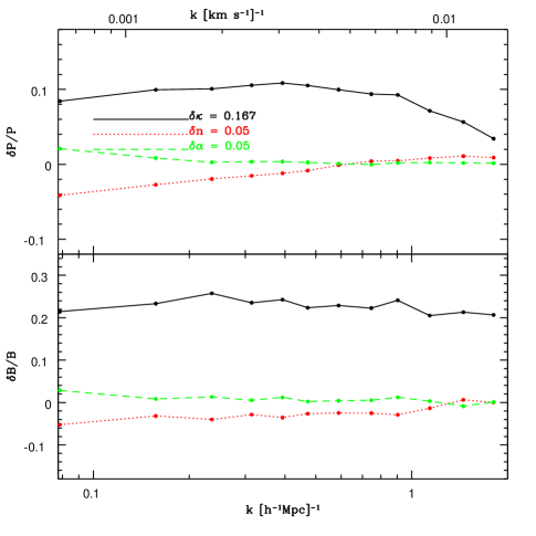
Figure 2: Plot of the relative variation of the statistics with $n$, $\alpha$, and $\kappa$ for one square filter.

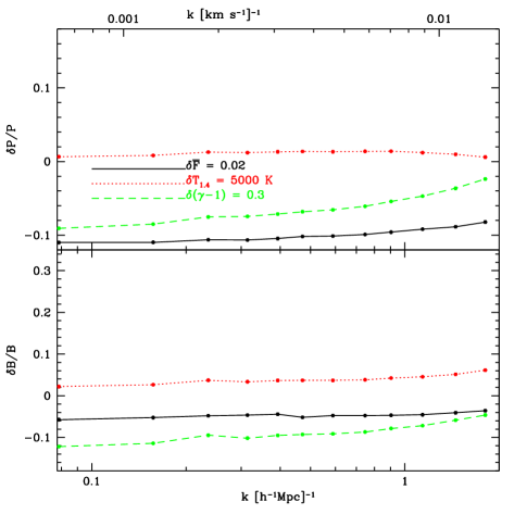
Figure 3: Plot of the relative variation of the statistics with $\bar{F}$, $\gamma-1$, and $T_{1.4}$.

We briefly explain the effects of changing the various parameters on $P$ and $B$ that are illustrated in Figs. 2 and 3. Raising the overall power spectrum amplitude causes an increase in $P$ and $B$ on all scales shown here, because the increase in power in the matter power spectrum carries directly over to the flux power spectrum. Increasing $n$ lowers $P$ and $B$ on large scales and raises it on small scales, directly reflecting its effects on the matter power spectrum (for even smaller scales than those shown here, increasing the power spectrum amplitude and $n$ actually causes a decrease in $P$ because non-linear peculiar velocities suppress power, as in McDonald (2001)). The statistics are nearly insensitive to $\alpha$ because it does not have much effect on these scales. $P$ and $B$ show only a very slight increase with $T_{1.4}$. The decrease of these statistics with an increase in $\gamma-1$, consistent with McDonald (2001), can be explained by considering the optical depth $\tau\propto\rho_{b}^{2-0.7(\gamma-1)}$, so that the exponent on $\rho_{b}$ is decreasing, and hence the fluctuations in optical depth for a given density fluctuation also decrease. The decrease in power with an increase in the mean flux is consistent with the results in McDonald (2001), and can be understood by the proportionality between the optical depth and $\rho_{b}^{2-0.7(\gamma-1)}$. Because the increased mean flux is equivalent to a lower optical depth, we can see that this should have the same effect as lowering the density fluctuations, and consequently the flux power spectrum (hence the degeneracy between power spectrum amplitude and mean flux).

2.2 Comparison of HPM and Hydro simulations

Fig. 4 shows the relative difference between HPM and hydrodynamic simulations at three redshifts, Fig. 5 shows their flux derivatives at $z=2.45$, and Fig. 6 shows their amplitude derivatives at $z=2.45$.

For the derivatives, the relative change (e.g., $\delta P/P$) was used for comparison, because differences in the magnitude of the derivatives could be simply artifacts of the differences in the magnitudes of the statistics themselves. Since this kind of change will cancel out of a Fisher matrix calculation (see equation 11), the relative change is plotted to emphasize changes in the $k$-dependent shape of the derivatives rather than their amplitude.

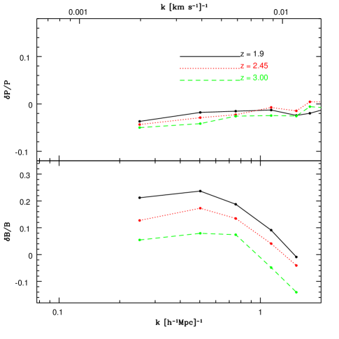
Figure 4: Relative difference in $P$ and $B$ for hydrodynamic vs. HPM simulations, for three $z$ values.

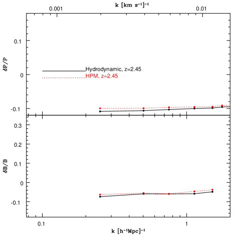
Figure 5: Relative difference in two-sided $\bar{F}$-derivatives hydrodynamic vs. HPM simulations, at $z=2.45$, with $\delta\bar{F}=0.02$.

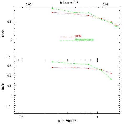
Figure 6: Comparison of amplitude derivatives for hydrodynamic vs. HPM simulations, with $\bar{F}=0.7$ and $\delta\kappa=0.167$.

As illustrated by Figs. 4-6, the HPM simulations yield statistics and derivatives fairly similar to those of the hydrodynamic simulations. The worst discrepancies in Fig. 4 occur for $z=1.9$, already below the range of this study. A Fisher matrix analysis using just amplitude and $\bar{F}$ was completed for these simulations, and found that the error bounds for both parameters were 6% lower when calculated with the HPM than with the hydro simulations, a tolerable difference for our purposes.

2.3 Resolution and box size

Another question about the HPM simulations is the box size and resolution necessary for a realistic study of these statistics. To check whether the 80 $h^{-1}$Mpc box with $512^{3}$ particles is sufficient, we computed the statistics and their derivatives for a 40 $h^{-1}$Mpc box with $512^{3}$ particles (higher resolution), and a 40 $h^{-1}$Mpc box with $256^{3}$ particles (same resolution, different box size). The values of the statistics and their derivatives with respect to $\bar{F}$ and $\kappa$ with $\gamma-1=0.3$, $T_{1.4}=17000$ K, $a=0.24$, $n=0.95$, $\alpha=0.0$, and $\bar{F}=0.7$, with typical instrumental effects, are in Figs. 7, 8, and 9, respectively. The filters are noted on the plot.

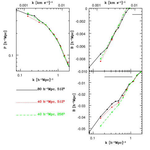
Figure 7: Comparison of statistics for different box size and resolution, with filters 0.2-1.1 $h^{-1}$Mpc (bottom) and 1.1-2.0 $h^{-1}$Mpc (top) as shown on plot.

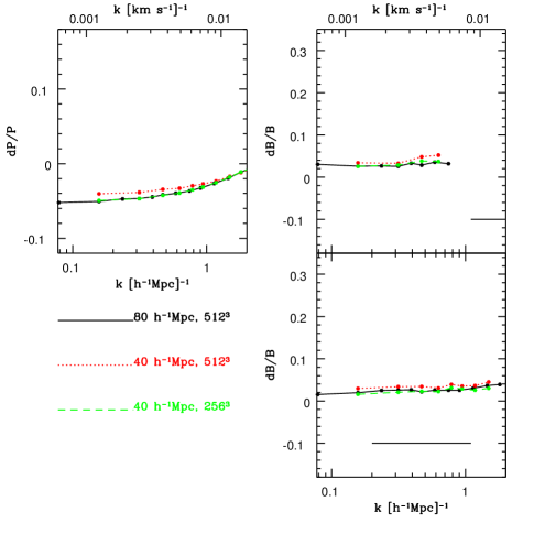
Figure 8: Comparison of $\bar{F}$-derivatives ($\delta\bar{F}=0.02$) for different box size and resolution, as noted on plot. The choice of filters for $B$ is the same as in previous plot.

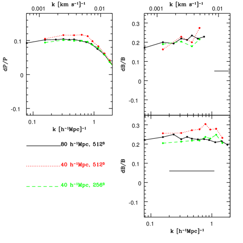
Figure 9: Comparison of $\kappa$-derivatives ($\delta\kappa=0.167$) for different box size and resolution, as noted on plot. The choice of filters for $B$ is the same as in previous plot.

As shown in Fig. 7, box size and resolution differences are generally within tolerance for $P$ and $B$ with the higher filter shown. Any small box size effects may be attributed to the difference in random seed in the 80 $h^{-1}$Mpc boxes versus the 40 $h^{-1}$Mpc boxes. There is a noticeable difference for $B$, the lower filter, between the higher and lower resolution 40 $h^{-1}$Mpc boxes. This difference cannot be attributed to a seed difference since the seed is same for these boxes. The difference is not evident between the 40 and 80 $h^{-1}$Mpc 512³ boxes, because of either a box-size effect or random fluctuations that oppose this resolution effect. For the most part, the $k$-dependent shapes of the derivatives agree, with the difference being one of magnitude. A smaller version of the Fisher analysis done in section 3 was completed for these boxes of different resolutions to check the effects of the derivative differences. The errors on amplitude are about 13% higher and on flux are about 15% lower with the lower resolution box than with the higher resolution box. However, since we are only looking at error bounds, which should hopefully be within about 25% accuracy, this error is tolerable, and the difference in Figure 7 is (by this criterion) not significant.

2.4 Random fluctuations due to finite box size

Another question is the magnitude of the random fluctuations due to finite box size, which can be determined by using different random seeds to generate the initial random Gaussian field. A study was done using three seeds, with $\gamma-1=0.3$, $T_{1.4}=17000$ K, $a=0.24$, $n=0.95$, $\alpha=0.0$, $\bar{F}=0.68$, and standard resolution and noise effects, on the values of $P$, $B$, and their $\bar{F}$- and $\kappa$-derivatives. Plots of the relative difference between the statistics and their $\bar{F}$-derivatives computed with individual seeds and averaged over three seeds are in Figs. 10 and 11 respectively. A plot of the relative difference between the statistics computed with individual seeds and averaged over four seeds for a 40 $h^{-1}$Mpc box is in Fig. 12.

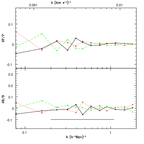
Figure 10: Relative difference between the values of the statistics computed with three different seeds and the average value (filter shown on plot) in an 80 $h^{-1}$Mpc box.

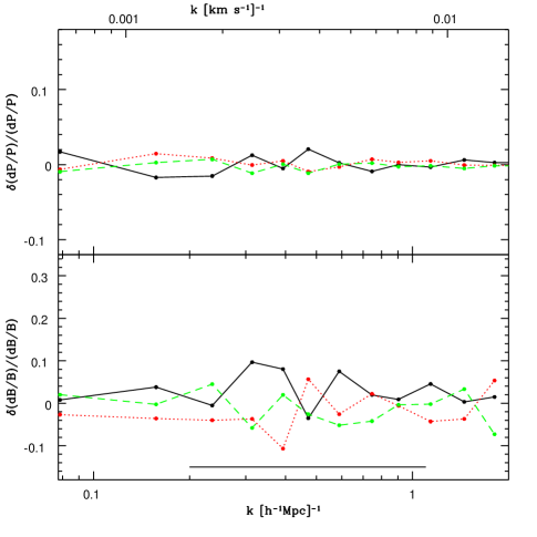
Figure 11: Relative difference between the values of $\bar{F}$-derivatives ($\delta\bar{F}$=0.02) computed with three different seeds and the averaged spectra (filter shown on plot) in an 80 $h^{-1}$Mpc box.

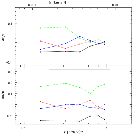
Figure 12: Relative difference between the values of the statistics computed with four different seeds and the average value (filter shown on plot) for a 40 $h^{-1}$Mpc box. The reason for the systematic difference between the $B$ values for different seeds is that these seeds gave higher or lower than average values of $P$ for several $k$, and since those $k$ were within the filter, that difference was spread systematically to all $k$.

As shown in these figures, the statistics and their derivatives for an 80 $h^{-1}$Mpc box do not have very large fluctuations due to finite box size, so only one random seed (the same each time, for consistency) was used for this analysis rather than averaging over the statistics obtained from several seeds. To check concretely that this is not a problem, a Fisher analysis for just $\kappa$ (derivatives not shown, but they have a similar pattern as the flux derivatives) and $\bar{F}$ at one $z$ was completed using three different seeds, and using the spectra and covariance matrices computed by averaging over lines of sight from all three seeds. The $\bar{F}$ and $\kappa$ error bounds for individual seeds were within 0.015 (relative difference) of the bounds for the averaged spectra. Note that the 40 $h^{-1}$Mpc box has significantly higher fluctuations, as expected, so it is possible that apparent box size effects are actually due to these fluctuations.

2.5 Chunking

The simulations were also used to study the effects of chunking, a procedure often used for data analysis. In the data, the spectra can be much longer than 80 $h^{-1}$Mpc, and are cut into smaller chunks for analysis. The fields $\delta_{F}(\lambda)$ and $H(\lambda)$ are both created from the full spectrum in real space before chunking.

To identify the effects of chunking, we compared the values of the statistics for an 80 $h^{-1}$Mpc box with $512^{3}$ particles; and the same 80 $h^{-1}$Mpc box, computed with half-lines of sight and averaged (see results in Fig. 13). All other simulation parameters were identical: $\gamma-1=0.3$, $T_{1.4}=17000$ K, $a=0.24$, $n=0.95$, $\alpha=0.0$, $\bar{F}=0.7$, and typical noise and resolution effects.

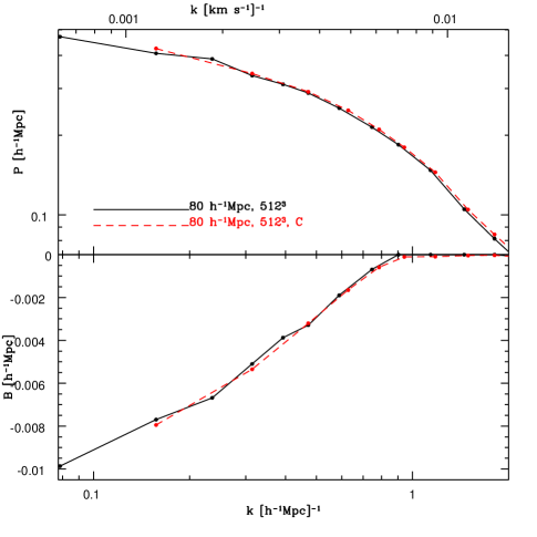
Figure 13: Plot of the statistics using full lines of sight from an 80 $h^{-1}$Mpc simulation, and a chunked 80 $h^{-1}$Mpc simulation. The code “C” refers to chunking.

As shown in Fig. 13, chunking has little effect on $P$ and $B$, with the values of the statistics computed using chunking almost perfectly matching those for the 80 $h^{-1}$Mpc box without chunking. Thus, the chunks of spectrum as small as 40 $h^{-1}$Mpc used in a data analysis can accurately represent the results in an infinite-spectrum limit.

2.6 Filters

As stated in section 2.1, we tried two filter shapes and several filter sizes and numbers of filters. The square window, in Eq. 6, was used in Zaldarriaga et al. (2001b). The Gaussian window was also tried since the Fourier transform of the square filter is not well-localized. The sizes of the filters were chosen based on the following consideration: the $k$ values in these 80 $h^{-1}$Mpc boxes range from 0.078-5.0 $h$Mpc^-1. Assuming $\Omega_{m}=0.3$, at $z=3$, this range corresponds to 0.0007-0.05 s km^-1. Below about 0.001 s km^-1, continuum fluctuations become important, and above about 0.02 s km^-1, resolution and noise effects become very important. Consequently, for square filters, the largest range of filter used is 0.002-0.02 s km^-1 (0.2-2.0 $h$Mpc^-1), and several smaller filters were chosen. For Gaussian filters, the question of filter width is a bit more difficult because there is some small contribution from beyond even $2\sigma$. Thus, we hoped to find the balance between the competing considerations of filter smoothness (compactness of the Fourier transform) versus its ability to eliminate $k$-values outside the range we want to consider. For the data, other possibly useful filters that can balance the smoothness and noise considerations are a triangular filter, or a Gaussian filter with a sharper low-$k$ cutoff. We show results for several sizes of square and Gaussian filters.

First we investigated how does an increase in number of filters with different sizes improve the information from $B$. A Fisher analysis using varying numbers of square filters was done to determine the number of filters to use in the range 0.2-2.0 $h$Mpc^-1. We tried using one or two filters by subdividing that interval accordingly. No filters overlapped, as analysis showed that overlap did not increase the amount of information at all. The error bars computed from one filter versus from two filters in the same range were within 5% of each other. Thus one filter is sufficient for analysis of a given range of $k$. However, for this analysis we used two non-overlapping filters for the total range, allowing us to analyze separately the information contribution of lower and higher filter ranges.

We also investigated filter sizes and shapes as shown in Table 1. Filter B1 is the lower filter of the pair referred to as filter B, and B2 is the higher filter. The numbers shown are actually for $z=3$; the filter parameters are constant in s km^-1, and so their value in $h$Mpc^-1 is $z$-dependent. While the magnitude of the statistics are rather filter-dependent, the shape of the statistics is essentially filter-independent and so the results were almost independent of the filter size and shape used, at least within the range of filters explored here.

	Filter 1		Filter 2
	Square Filters
	Start	End	Start	End
B	0.2	1.1	1.1	2.0
C	0.4	1.2	1.2	2.0
D	0.2	1.0	1.0	1.8
E	0.4	1.1	1.1	1.8
	Gaussian Filters
	$\bar{k}$	$\sigma_{k}$	$\bar{k}$	$\sigma_{k}$
F	0.65	0.2	1.5	0.3
G	0.65	0.13	1.5	0.2
H	0.65	0.27	1.5	0.4

Table 1: Table of codes for the seven filters analyzed. All figures are in $h$Mpc^-1 at $z=3$.

2.7 Instrumental dependencies

Noise and resolution play an important role in determining the sensitivity of a given data set. We parameterize the noise with two numbers, $f_{c}$ (the fraction of noise whose amplitude is correlated with the signal) and $S/N$ (the overall signal to noise ratio relative to the continuum, including all noise). Noise whose amplitude is correlated with the signal is characterized by its variance $\sigma_{c}^{2}=c\bar{F}$ (where $\bar{F}$ is the mean flux from the quasar). A typical example is photon shot noise, where the variance is proportional to the flux. Noise whose amplitude is uncorrelated with the signal is characterized by its variance $\sigma_{u}^{2}$ (for example, Gaussian readout noise and photon shot noise from the sky) These variables are related as follows, defining a unique $c$ and $\sigma_{u}^{2}$ for each $f_{c}$ and $S/N$:

$$f_{c} =\frac{c\bar{F}}{c\bar{F}+\sigma_{u}^{2}}$$ (9)

$$S/N =\frac{1}{\sigma_{f}}=\frac{1}{\sqrt{\sigma_{u}^{2}+c\bar{F}}}$$ (10)

The distinction between correlated and uncorrelated noise amplitude is made because they have different effects on $B$ and $T$. Uncorrelated noise contributes to $P$ and $T$, but not to $B$, whereas correlated noise contributes to all three. The noise’s contribution to $P$ can be calculated analytically whether its amplitude is correlated or uncorrelated with the signal. The correlated noise contribution to $B$ depends not only on the noise amplitude, but also on the signal power spectrum $P$.

In this study, we tried to match the pixelization, resolution, and noise to that of the SDSS data. The pixels in SDSS data are roughly 1 Å wide (so the smoothing $\sigma$ is approximately the size of one pixel). Assuming $z=3$ and $\Omega_{m}=0.3$ this corresponds to 0.6 $h^{-1}$Mpc. To match the 0.6 $h^{-1}$Mpc pixels, we used pixels of size 0.625 $h^{-1}$Mpc in the simulations. This small difference from the real value makes little effect in the value of the statistics, since even reducing the pixel size by a factor of four changes $B$ and $P$ by at most 5%. We used Gaussian smoothing $\sigma$ the same size as our pixels. SDSS data have $S/N$ (averaged over redshift bins in our range) ranging from 1 to 30, with median values in each redshift bin ranging from 4 to 5. We used the value $S/N=5.0$ for all redshift bins. The noise amplitude was entirely uncorrelated with the signal ($f_{c}=0$), since we could not evaluate the amount of correlated noise in the data.

3 Fisher Matrix Calculation and Results

The construction of the Fisher matrices for each individual redshift bin is straightforward. A vector containing all values $x_{i}$ that were to be used (for example, $P$ and $B$ for all $k$) was created, as was its full covariance matrix (computed using all 12288 lines of sight) and its derivatives with respect to the 6 parameters $\gamma$, $T_{1.4}$, $\kappa$, $n$, $\alpha$, and $\bar{F}$. The derivatives with respect to $P$ were created from the values with the power due to noise subtracted off. These covariance matrices and derivatives were then used to create the $6\times 6$ Fisher matrices for each redshift bin by computing

$$F_{kl}=\left(\frac{\mathrm{d}\mathbf{x}}{\mathrm{d}y_{k}}\right)^{T}\cdot\mathsf{C}^{-1}\cdot\left(\frac{\mathrm{d}\mathbf{x}}{\mathrm{d}y_{l}}\right)$$ (11)

so that $\mathsf{F}$ is the inverse covariance matrix for $\mathbf{y}$, the vector of all the parameters. In general, there is another term related to $\mathrm{d}\mathsf{C}/\mathrm{d}y_{i}$ that we neglect in the expectation that it is small.

Next, a block-diagonal $54\times 54$ Fisher matrix was created, using the $6\times 6$ Fisher matrices for the nine redshift bins. Each block was multiplied by the length of spectrum in that redshift bin in the SDSS data; the total spectrum length is $7.7\times 10^{7}$ km/s. Fisher matrices in this form were created for all seven sets of filters listed in Table 1, for various combinations of statistics. Further information about error-bounds is extracted from these large Fisher matrices by projecting from them down to a smaller number of parameters.

3.1 Projection to fewer parameters

To reduce to the smallest number of parameters, we used the following procedure. The $54\times 54$ Fisher matrices are the inverse covariance matrices $\mathsf{C}^{-1}(\mathbf{y})$ for the values of the parameters in each redshift bin. We projected down to a smaller set of parameters that includes:

• $\gamma_{0}$ and $\gamma_{1}$, the constant and linear terms of a linear expansion of $\gamma(z)$ about $z=3.0$,

• $T_{1.4}$, an overall redshift-independent value,

• $\kappa_{\mathrm{eff}}$, an overall effective amplitude at some $z$ and $k$,

• $n_{\mathrm{eff}}$, an overall effective slope, where the evolution of the pivot point (fixed in velocity coordinates) is expressed via $n(z)=n(k_{p})+\alpha\ln{(k_{p}(z)/k_{p})}$,

• $\alpha_{\mathrm{eff}}$, an overall effective curvature, and

• The nine values of $\bar{F}$, one per redshift bin.

This projection includes 15 parameters, and can be computed using Eq. 11.

Here we present results for the analysis done with just filter B, using $P$ and $B$. All references to “error bounds” implies that we have marginalized over other parameters (by using $\sqrt{(F^{-1})_{ii}}$ rather than $1/\sqrt{F_{ii}}$).

First, the error bounds for $\gamma_{0}$ and $\gamma_{1}$, defined by [$\gamma-1](z)=\gamma_{0}+\gamma_{1}(z-3)$, are 0.054 and 0.10, respectively. We are not very sensitive to $T_{1.4}$, with a relative error of 0.08.

Table 2 shows the relative errors for the nine values of $\bar{F}$. The errors increase with redshift mainly because the amount of data decreases, and at low redshifts they are extremely small.

$z$	$\bar{F}$	$\Delta\bar{F}/\bar{F}$
2.2	0.85	0.0030
2.4	0.81	0.0035
2.6	0.77	0.0033
2.8	0.73	0.0036
3.0	0.68	0.0046
3.2	0.63	0.0057
3.4	0.57	0.0075
3.6	0.52	0.011
3.8	0.46	0.015

Table 2: Error bounds on $\bar{F}(z)$ using $P$ and $B$.

The error on $\kappa=(\Delta\sqrt{A})/\sqrt{A}$ is .017. The errors on $n_{\mathrm{eff}}$ and $\alpha_{\mathrm{eff}}$ (defined at pivot point $k=0.009$ s km^-1 at $z=2.6$) are $\Delta n_{\mathrm{eff}}=0.013$, and $\Delta\alpha_{\mathrm{eff}}=0.029$. The error ellipse in terms of $n_{\mathrm{eff}}$ and $\alpha_{\mathrm{eff}}$ computed from their joint covariance matrix is in Fig. 14. To answer the question of whether $B$ alone provides independent information competitive wih $P$, or whether $B$ and $P$ together is more sensitive than either of the two alone, we carried out the analysis using $P$ alone, $B$ alone, and $P$ and $B$ together. The error bounds for all parameters for various combinations of statistics can be found in Table 3.

	$P$	$B$	$PB$
$\Delta\gamma_{0}$	0.097	0.086	0.054
$\Delta\gamma_{1}$	0.18	0.17	0.10
$\Delta T_{1.4}/T_{1.4}$	0.096	0.093	0.081
$\Delta\kappa_{\mathrm{eff}}$	0.045	0.035	0.017
$\Delta n_{\mathrm{eff}}$	0.014	0.058	0.013
$\Delta\alpha_{\mathrm{eff}}$	0.037	0.063	0.029
$\Delta\bar{F}_{1}/\bar{F}_{1}$	0.0082	0.0057	0.0030

Table 3: Errors using various combinations of statistics (note that $\bar{F}_{1}$ is the mean flux for the first redshift bin, and illustrates the trend in errorbars for all mean fluxes).

Fig. 14 shows the 68% confidence level error ellipses for $n_{\mathrm{eff}}$ and $\alpha_{\mathrm{eff}}$ for $P$, $B$, and both together. It is clear that for this combination of parameters $P$ provides most of the information. While $B$ can act as a useful independent confirmation, adding its information by itself does not decrease the statistical errors significantly.

Fig. 15 shows the 68% CL error ellipses for $\kappa_{\mathrm{eff}}$ and $\bar{F}(z=3.0)$ for $P$, $B$, and both together. In contrast with Fig. 14, combining the two significantly improves upon $P$ or $B$ alone, reducing the errors on $\kappa$ and $\bar{F}$ by almost a factor of 3. The primary reason for this is the partial degeneracy between the two parameters in $P$ alone, as shown in Fig. 15. This degeneracy is easy to understand from the derivatives in Figs. 2 and 3. Changing $\kappa$ or $\bar{F}$ has a relatively flat effect on the power spectrum $P$, so the two parameters are significantly degenerate from $P$ alone, especially when all the other parameters are included. In contrast, the effect on $B$ is much larger for $\kappa$ than for $\bar{F}$. Combining $P$ and $B$ thus allows one to break the degeneracy between the two parameters and determine both with a much higher precision.

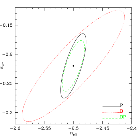
Figure 14: 68% CL error ellipses for $n_{\mathrm{eff}}$ and $\alpha_{\mathrm{eff}}$ computed with various combinations of statistics.

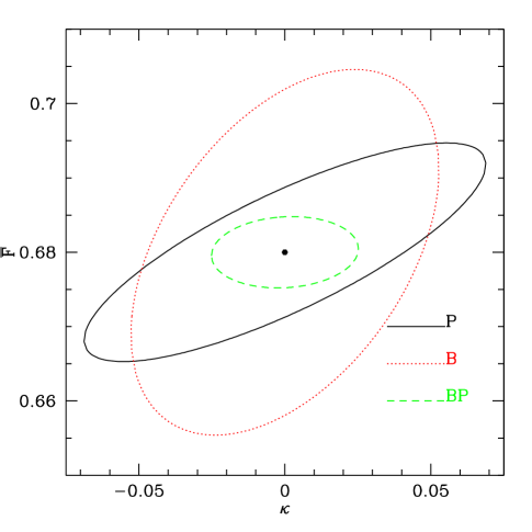
Figure 15: 68% CL error ellipses for $\kappa_{\mathrm{eff}}$ and $\bar{F}(z=3)$ computed with various combinations of statistics. Note that the correlation coefficient between these parameters is 0.80 for $P$, 0.45 for $B$, and 0.10 for $B$ and $P$ together. The reason that the correlation is so reduced when $B$ and $P$ are used together is that there are nonzero covariance matrix elements between $B$ and $P$ at the same $k$, so the Fisher matrix is not that produced by simply adding those for $B$ and $P$ together.

We also investigated how the errors vary with filter, finding that they did not vary significantly for filters given in Table 1. In particular, the error bounds on $n_{\mathrm{eff}}$ and $\alpha_{\mathrm{eff}}$ were virtually independent of filter, and those on $\kappa_{\mathrm{eff}}$ were nearly so. Among the Gaussian filters, there was a slight trend towards lower error bounds on $\kappa_{\mathrm{eff}}$ for the larger filters (0.015 for the largest versus 0.018 for the smallest) but even here the difference is not very large.

3.2 Expansions of $\kappa_{\mathrm{eff}}$, $n_{\mathrm{eff}}$, and $\alpha_{\mathrm{eff}}$

In order to determine how much variation in the values of $n_{\mathrm{eff}}$, $\alpha_{\mathrm{eff}}$, and $\kappa_{\mathrm{eff}}$ (at a particular $z$ and $k$) is induced by deviations in $n$, $\alpha$, $\Omega_{m}$, $\Omega_{b}$, and $h$, we used CMBFAST (Seljak & Zaldarriaga, 1996) outputs to study the derivatives with respect to these parameters, using spectra that were normalized to the same amplitude at $k=0.05$ $h$Mpc^-1 at $z=20$. The derivatives were computed at $z=2.6$, $k=0.009$ s km^-1, the pivot point for SDSS data sample. We assume the fiducial model $\Omega_{m}=0.3$, $h=0.7$, $\Omega_{b}=0.04$ (or $x\equiv\Omega_{b}/\Omega_{m}=0.13$). The pivot point for $\alpha$ is $k=0.05$ $h$Mpc^-1. The expansion for $\kappa_{\mathrm{eff}}$ is denoted $\Delta\kappa_{\mathrm{eff}}$ to emphasize that this expansion is to be used to calculate what relative change in power spectrum amplitude would result from changing the cosmological parameters from our chosen values (hence it gives $\Delta\kappa_{\mathrm{eff}}=0$ for our cosmological model). The resulting expansions are

$$\Delta\kappa_{\mathrm{eff}} =\Delta\kappa+1.5(n-0.75)-0.032\alpha$$ (12)

$$\quad+0.28\ln{\left(\frac{\Omega_{m}}{0.3}\right)}+0.65\ln{\left(\frac{h}{0.7}\right)}+0.14\ln{\left(\frac{x}{0.13}\right)}$$

$$n_{\mathrm{eff}} =-3.25+n+3.0\alpha+$$ (13)

$$\quad 0.16\ln{\left(\frac{\Omega_{m}}{0.3}\right)}+0.23\ln{\left(\frac{h}{0.7}\right)}+0.034\ln{\left(\frac{x}{0.13}\right)}$$

$$\alpha_{\mathrm{eff}} =-0.22+\alpha-0.11\ln{\left(\frac{\Omega_{m}}{0.3}\right)}$$ (14)

$$\quad-0.17\ln{\left(\frac{h}{0.7}\right)}+0.034\ln{\left(\frac{x}{0.13}\right)}$$

The effect on the amplitude is primarily determined by the primordial amplitude and slope, but not the derivative of the slope (given that the pivot point $k=0.05$ $h$Mpc^-1 is at much lower $k$ than the wavevectors the forest is sensitive to). Today’s matter density $\Omega_{m}$ and Hubble constant $h=H_{0}/100$ ${\rm km/s/Mpc}$ change the transfer function and so affect the amplitude, slope and derivative of the slope. However, $\Omega_{m}$ also changes the relation between velocities and comoving coordinates as given by the Hubble parameter $H(z)$. This partially cancels the transfer function effect of $\Omega_{m}$, so that the coefficients in front of $\Omega_{m}$ are reduced relative to $h$. Baryon density has a smaller effect than other parameters, at least around the small value of $\Omega_{b}/\Omega_{m}$ we expanded here.

It is clear that since we can only determine precisely two numbers, the amplitude and the slope, and somewhat less precisely also the derivative of the slope, we cannot determine all of the parameters with high precision. Hence it is best if the Ly-$\alpha$ forest is combined with other cosmological probes, such as cosmic microwave background (CMB) anisotropies. Since one expects CMB to provide very strong constraints on $h$ and $\Omega_{m}$ (at least in the context of spatially flat models), this then allows the Ly-$\alpha$ forest to determine the primordial slope and its derivative with high accuracy.

4 Power Spectrum Evolution and Quintessence

In this section we try to determine the sensitivity of the Lyman-$\alpha$ forest to deviations from the Einstein-de Sitter (EdS) growth factor $D(a)=a$. We analyzed both specific quintessence models and also more general deviations of the growth factor from EdS. Sensitivity to quintessence model parameters can arise from the change in the growth factor $D(z)$ and from the Hubble parameter $H(z)$. In our tests the latter was subdominant and most of the sensitivity was from the growth factor.

First, we studied the sensitivity of the Lyman-$\alpha$ forest to quintessence parameters, $\Omega_{q}$ and the equation of state $w_{q}$, for nine different quintessence models. Several models considered had static equation of state $w_{q}=w_{0}$, while the other models were dynamic, $w_{q}=w_{0}+w_{1}(a-1)$. The models studied are shown in Table 4.

Model	$\Omega_{q,0}$	$\Omega_{q}(z=2.6)$	$w_{0}$	$w_{1}$
1	0.67	0.12	-0.7	0.0
2	0.85	0.28	-0.7	0.0
3	0.49	0.06	-0.7	0.0
4	0.67	0.04	-1.0	0.0
5	0.67	0.30	-0.4	0.0
6	0.67	0.12	-0.8	-0.2
7	0.67	0.19	-0.8	-0.5
8	0.67	0.27	-0.8	-0.8
9	0.67	0.09	-1.0	-0.5

Table 4: Codes for quintessence models, where $w_{q}=w_{0}+w_{1}(a-1)$.

All models had $\Omega_{b}=0.04$ and $h=0.7$, with $\Omega_{\mathrm{CDM}}$ determined by requiring $\Omega_{b}+\Omega_{\mathrm{CDM}}+\Omega_{q}=1$.

4.1 Projection with quintessence parameters

To find constraints on all parameters once quintessence parameters are included, we started from the $54\times 54$ Fisher matrices created in section 3, and projected down to the parameters in section 3.1 plus $\Omega_{q}$ and $w_{q}$ (or $\Omega_{q}$, $w_{0}$, and $w_{1}$ for dynamical models). All error bounds are computed from the Fisher matrix for filter B using $P$ and $B$. To do so, we computed derivatives of $\kappa_{\mathrm{eff}}$, $n_{\mathrm{eff}}$, and $\alpha_{\mathrm{eff}}$ with respect to quintessence parameters at some pivot point fixed in s km^-1. These derivatives were computed from CMBFAST outputs for the 9 $z$-bins for all 9 quintessence models studied, normalized to have the same amplitude for $z=20$ at the same pivot point at which derivatives were taken.

Results for all models indicated that $w_{q}$ and $\Omega_{q}$ are highly degenerate, with a correlation coefficient of -0.9. The well-determined direction for model 1, which is fairly representative, in $(w_{q},\Omega_{q})$ space is $(0.60,0.80)$. The strong correlation is not surprising, since the redshift range probed is too small to determine two parameters from the growth factor or $H(z)$ evolution. Some information on $\Omega_{q}$ also comes from the power spectrum shape, which is why the correlation is not perfect. In the following we thus fix one parameter, for example $\Omega_{q}$, and present errors on equation of state only. The motivation for this is that other tests, most notably CMB combined with large scale structure tests (e.g. cluster counts, galaxy clustering, weak lensing), will be able to determine $\Omega_{q}$ at $z=0$ very accurately. If these tests also provide independent constraints on $w_{0}$ then for the time dependent $w$ one can use our results to constrain $w_{1}$.

The errors for fixed $w_{q}$ (marginalized over all other variables) can be found in Table 5. The 68% CL error ellipses show how $\Omega_{q}$ and amplitude are degenerate (Fig. 16). Analysis of the covariance matrices for these model parameters (or the fact that the error bounds for $\kappa_{\mathrm{eff}}$, $n_{\mathrm{eff}}$, and $\alpha_{\mathrm{eff}}$ have risen from their value computed without including quintessence) indicated a very high degree of degeneracy between $\Omega_{q}$ and $\kappa_{\mathrm{eff}}$, $n_{\mathrm{eff}}$, and $\alpha_{\mathrm{eff}}$. If $\alpha$ is fixed then the errors on $\Omega_{q}$ consequently decrease (though this effect is much greater for the models to which we are least sensitive). This indicates that at least some of our information about quintessence parameters comes from shape information. The degeneracy with $\kappa_{\mathrm{eff}}$ indicates that some information is from the growth factor information as well, since the magnitude of the growth factor (as opposed to its shape) is degenerate with $\kappa_{\mathrm{eff}}$. The errors with $w$ and $\alpha$ fixed are in Table 6.

Model	$\Delta\Omega_{q}/\Omega_{q}$	$\Delta\kappa_{\mathrm{eff}}$	$\Delta n_{\mathrm{eff}}$	$\Delta\alpha_{\mathrm{eff}}$
1	0.26	0.041	0.057	0.052
2	0.05	0.073	0.047	0.034
3	0.48	0.028	0.075	0.053
4	0.31	0.017	0.097	0.078
5	0.13	0.025	0.049	0.038
6	0.16	0.037	0.053	0.049
7	0.11	0.048	0.040	0.039
8	0.09	0.063	0.035	0.033
9	0.20	0.030	0.066	0.052

Table 5: Error bounds for all quintessence models with fixed equation of state, marginalized over other parameters.

Model	$\Delta\Omega_{q}/\Omega_{q}$	$\Delta\kappa_{\mathrm{eff}}$	$\Delta n_{\mathrm{eff}}$
1	0.14	0.024	0.039
2	0.04	0.059	0.043
3	0.26	0.018	0.049
4	0.11	0.017	0.043
5	0.10	0.019	0.041
6	0.09	0.022	0.037
7	0.08	0.034	0.034
8	0.08	0.051	0.033
9	0.11	0.019	0.044

Table 6: Error bounds for all quintessence models with fixed equation of state and $\alpha$, marginalized over other parameters.

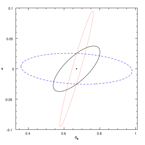
Figure 16: 68% CL error ellipse for $\Omega_{q}$ and amplitude, with $w_{q}$ (but not $\alpha_{\mathrm{eff}}$) fixed, for cosmological constant (model 4) as dashed lines, quintessence with $w=-0.4$ (model 5) as solid lines, and a dynamic quintessence model (model 8) as dotted lines.

Error bounds on $w_{q}$ for static models, with $\Omega_{q}$ fixed (as may be done by measurements other than the Lyman-$\alpha$ forest), are shown in Table 7. As shown there, now that $\Omega_{q}$ is fixed, $n_{\mathrm{eff}}$ and $\alpha_{\mathrm{eff}}$ have error bounds roughly equal to those computed in the previous section with no quintessence. This fact shows that these parameters contain information about $\Omega_{q}$ but not $w_{q}$. $\kappa_{\mathrm{eff}}$, on the other hand, is degenerate with $w_{q}$, indicating that $w_{q}$ is detected via its influence on the growth factor. Consequently, the model with least negative $w_{q}$ has the best error bounds. Table 8 shows error bounds for $w_{1}$ with both $\Omega_{q}$ and $w_{0}$ fixed. Errors for $n_{\mathrm{eff}}$ and $\alpha_{\mathrm{eff}}$ are not shown since they are the same as in the previous section, without quintessence. Not surprisingly, the error bounds are best for the model with the most rapidly-varying equation of state.

Model	$\Delta w_{q}$	$\Delta\kappa_{\mathrm{eff}}$	$\Delta n_{\mathrm{eff}}$	$\Delta\alpha_{\mathrm{eff}}$
1	0.22	0.10	0.016	0.029
2	0.09	0.10	0.014	0.028
3	0.36	0.08	0.016	0.029
4	0.36	0.06	0.013	0.029
5	0.17	0.25	0.025	0.028

Table 7: Error bounds for static quintessence models with fixed $\Omega_{q}$, marginalized over other parameters.

Model	$\Delta w_{1}$	$\Delta\kappa_{\mathrm{eff}}$
6	0.31	0.06
7	0.22	0.07
8	0.18	0.08
9	0.41	0.06

Table 8: Error bounds for dynamic quintessence models with fixed $\Omega_{q}$ and $w_{0}$, marginalized over other parameters.

4.2 More general growth

Besides considering specific quintessence models, we also considered more general power spectrum evolution, modeled as

$$D(a)=D_{0}(a/a_{0})^{s},$$ (15)

where $s=1$ corresponds to an Einstein-de Sitter universe. Thus, we can determine if our sensitivity to quintessence is due to growth factor deviations. This analysis was completed by starting with the $54\times 54$ Fisher matrix for $P$ and $B$ (filter B), and projecting down to the same set of parameters as in Section 3.1 along with $s$. The projection for $\kappa$ and $s$ used $P\propto e^{2\kappa}D^{2}(a)$ to relate the necessary derivatives $\mathrm{d}P/\mathrm{d}\kappa$ and $\mathrm{d}P/\mathrm{d}s$ to the computed values $\mathrm{d}P/\mathrm{d}a$. Using the value of $a_{0}$ determined by requiring that amplitude and $s$ have the minimum degeneracy, and inputting a value of $s=1$, yields an error $\Delta s=0.11$. Note that if only information from the power spectrum $P$ is used (rather than including $B$ as done here), the error rises to $\Delta s=0.47$.

Values of $\Delta s$ for arbitrary static quintessence models were computed using an integral expression for $D(a)$ obtained from Hamilton (2001), Taylor expanding to several orders, which gave a form $D(a)=a\left(1+\sum_{n=1}c_{n}(\Omega_{q},w_{q})a^{-3nw_{q}}\right)$. Expanding this expression about $a_{0}$ gave an expression for $s$, and hence for $\Delta s=s-1$, in terms of the model parameters. Requiring $|\Delta s|<0.11$ defines the region in $w_{q}$-$\Omega_{q}$ parameter space that is detectable using the Lyman-$\alpha$ forest (growth factor information only, not curvature). This curve is shown in Fig. 17.

Figure 17: Curve in the $\Omega_{q}$, $w_{q}$ plane indicating regions for which the deviation from $D(a)=a$ would be detectable using growth factor information (1 and $2\sigma$ as solid and dashed lines, respectively). Note that the Gaussian approximation is worse for the $2\sigma$ errors.

To check the validity of this expansion, the growth factor was computed directly from CMBFAST outputs for the 9 quintessence models studied above. This also allowed the computation of $\Delta s$ for dynamic models, for which an analytic expression was not obtained. Values of $\Delta s$ for the 9 models studied earlier, and values of $\Omega_{q}(z=2.6)$, are shown in Table 9. As shown, $\Delta s$ and $\Omega_{q}(z=2.6)$ are highly correlated.

Model	$\Omega_{q}(z=2.6)$	$\Delta s$	Detect?
1	0.12	-0.085	No
2	0.28	-0.22	Yes
3	0.06	-0.042	No
4	0.04	-0.024	No
5	0.30	-0.23	Yes
6	0.12	-0.082	No
7	0.19	-0.14	Yes
8	0.27	-0.22	Yes
9	0.09	-0.060	No

Table 9: Values of $\Delta s$ for the nine quintessence models, where detectability of growth factor deviation is defined by $|\Delta s|>0.11$.

4.3 Change in $H(z)$

So far the only tests of dark energy proposed have used either the growth factor or the redshift luminosity distance. If one wishes to extract $w(z)$, then both of these involve a double integral over this quantity and degeneracies arise. A more direct and still in principle observable way is to measure the Hubble parameter $H(z)$, which is related to $w(z)$ through a single integral. One way to measure it is to have a characteristic feature fixed in comoving coordinates which is observed in redshift space. The relation between redshift space and comoving space is determined by $H(z)$ and so observing the feature as a function of redshift determines its evolution. The problem of course is that there are no characteristic features imprinted, since the distribution of structure in the universe is stochastic in nature.

One must therefore look for a characteristic scale in correlations between structures. In principle such features could be provided by baryonic oscillations imprinted in the matter power spectrum, but in practice this is a weak effect limited to very large scales and so cannot be made very precise. One is thus left with the variations in the correlation function slope as a function of scale. The slope varies from $n\sim 1$ on large scales to $n\sim-3$; on Ly-$\alpha$ forest scales we find $\alpha_{\rm eff}=-0.22$ in CDM models. Hence the scale at which the slope takes a specific value can be viewed as a standard ruler and can be traced with redshift. If this slope is measured in redshift space, then one is measuring directly $H(z)$. To be able to do this one has to detect the curvature in the slope over the dynamic range of observations. This is challenging, since the dynamic range is narrow and the error on the slope will be large. We find that such a detection should be possible with the current sample, but is not expected to improve the constraints on $w(z)$ significantly.

5 Discussion and Conclusions

Our results show that the statistical precision one can achieve from Ly-$\alpha$ forest using SDSS data is truly impressive. The overall amplitude of the power spectrum, its slope and its curvature can all be determined with 1-3% precision. Our results are significantly more optimistic than those in Zaldarriaga et al. (2001a), which focused on a higher resolution but smaller data sample available from Keck. This is primarily a consequence of the large sample size of SDSS data, which increases the statistical precision on larger scales and moves the pivot point from $0.03$ to $0.01$ s km^-1. On larger scales the sensitivity of the power spectrum to the gas temperature-density relation is reduced so one is measuring more directly the underlying matter power spectrum. In addition, we have shown here that higher order correlations break the degeneracy between the mean flux and the amplitude (this degeneracy is broken to some extent already by the power spectrum alone). Using the power spectrum alone and the bispectrum alone are two independent ways to confirm this determination. Using them together gives even lower error bounds due to the breaking of degeneracies. The statistical precision of such a data set is competitive with the one from the CMB using the MAP and Planck satellites. More importantly, combining the two probes will allow one to determine the primordial power spectrum to a high precision over 3 decades in scale ($0.001<k<2$ $h$Mpc^-1).

Furthermore, since one is measuring the power spectrum over a range of redshifts ($2<z<4$), one can also study the growth factor evolution. While for standard cosmological constant models the universe is effectively Einstein-de Sitter for $z>2$, dynamical models with rolling scalar fields often produce an equation of state increasing with redshift (this is especially true for many of the so-called tracker models). In this case the dark energy or quintessence is still dynamically important for $z>2$ and can affect the growth rate of perturbations and the Hubble parameter $H(z)$. While there is no simple single parameter combination that describes the sensitivity to dark energy, it is clear that the precision is correlated with $\Omega_{q}$ at $z>2$. Our results show that if $\Omega_{q}(z=2.6)>0.2$ then the deviations in the growth factor are sufficiently large to be detected in Ly-$\alpha$ forest spectra using the current SDSS sample. With the full SDSS sample this limit can be improved further and models with $\Omega_{q}(z=2.6)>0.1$ should be detectable. This sensitivity can increase further if one can extend the available data set to even lower redshifts by using space based observations.

While it is clear that the statistical power of upcoming data sets is impressive, the main remaining issue is whether the simplest model of the QSO absorption adopted here is valid, or whether there are other more complicated astrophysical processes that can spoil the picture. Since the expected statistical precision is so high one must investigate processes that affect the statistics even at a very small (1%) level. There are several possible complications that may have an effect and we mention some here: metal line absorption along the line of sight (e.g. C-IV, Si-III…), an inhomogeneous UV background, kinematic gas outflows generated by supernovae from the galaxies, temperature fluctuations, etc.

Fortunately, while there are several possible contaminations, there are also several possible tests one can apply to identify and remove the contamination. Some of these processes can be investigated with the statistics used in this paper, such as the power spectrum and bispectrum. In the simplest model the main driver of correlations is gravity, which induces a very specific relation between low and higher order statistics. Any astrophysical contamination is likely to destroy these relations. Other tests such as the probability distribution of the flux (as a function of scale) will also yield useful information (McDonald et al., 2000). Another way to investigate these effects is through the cross-correlation between the forest and galaxies at the same redshift (Adelberger et al., 2003); for theoretical attempts to interpret this result, see McDonald et al. (2002), Croft et al. (2002a), Kollmeier et al. (2002) and Bruscoli et al. (2002).

If the simplest model passes this and other high precision tests it will receive an important confirmation that will strengthen the credibility of the results. In the opposite case one can still identify the contaminant and apply the corrections assuming the contamination is sufficiently well understood. This parallels the situation in the CMB, where secondary processes and foregrounds are searched for and, if identified, subtracted from the primary CMB. It is clear however that a validation of the interpretation set forth by the simplest model will require a lot of coordinated effort from several groups and more effort should be put into this. Our results suggest that this is well worth the effort and that the Ly-$\alpha$ forest could be our next cosmological gold-mine.

R.M. is supported by an NSF Graduate Research Fellowship. This work was supported by NASA, NSF CAREER, David and Lucille Packard Foundation and Alfred P. Sloan Foundation. We thank Nick Gnedin for the HPM code. The simulations were performed at the National Center for Supercomputing Applications.

References

- Adelberger et al. (2003) Adelberger K. L., Steidel C. C., Shapley A. E., Pettini M., 2003, ApJ, 584, 45
- Bruscoli et al. (2002) Bruscoli M., Ferrara A., Marri S., Schneider R., Maselli A., Rollinde E., Aracil B., 2002
- Cen & McDonald (2002) Cen R., McDonald P., 2002, ApJ, 570, 457
- Cen et al. (1994) Cen R., Miralda-Escude J., Ostriker J. P., Rauch M., 1994, ApJ, 437, L9
- Cen et al. (2002) Cen R., Ostriker J. P., Prochaska J. X., Wolfe A. M., 2002, ApJ, submitted (astro-ph/0203524)
- Cen et al. (2001) Cen R., Tripp T. M., Ostriker J. P., Jenkins E. B., 2001, ApJ, 559, L5
- Croft et al. (2002a) Croft R. A. C., Hernquist L., Springel V., Westover M., White M., 2002a, ApJ, 580, 634
- Croft et al. (2002b) Croft R. A. C., Weinberg D. H., Bolte M., Burles S., Hernquist L., Katz N., Kirkman D., Tytler D., 2002b, ApJ, 581, 20
- Croft et al. (1998) Croft R. A. C., Weinberg D. H., Katz N., Hernquist L., 1998, ApJ, 495, 44
- Croft et al. (1999) Croft R. A. C., Weinberg D. H., Pettini M., Hernquist L., Katz N., 1999, ApJ, 520, 1
- Gnedin & Hui (1998) Gnedin N. Y., Hui L., 1998, MNRAS, 296, 44
- Hamilton (2001) Hamilton A. J. S., 2001, MNRAS, 322, 419
- Hernquist et al. (1996) Hernquist L., Katz N., Weinberg D. H., Jordi M., 1996, ApJ, 457, L51
- Hui et al. (2001) Hui L., Burles S., Seljak U., Rutledge R. E., Magnier E., Tytler D., 2001, ApJ, 552, 15
- Kollmeier et al. (2002) Kollmeier J. A., Weinberg D. H., Dave’ R., Katz N., 2002, ArXiv Astrophysics e-prints, 12355
- McDonald (2001) McDonald P., 2001, ApJ, in press (astro-ph/0108064)
- McDonald et al. (2002) McDonald P., Miralda-Escudé J., Cen R., 2002, ApJ, 580, 42
- McDonald et al. (2001) McDonald P., Miralda-Escudé J., Rauch M., Sargent W. L. W., Barlow T. A., Cen R., 2001, ApJ, 562, 52
- McDonald et al. (2000) McDonald P., Miralda-Escudé J., Rauch M., Sargent W. L. W., Barlow T. A., Cen R., Ostriker J. P., 2000, ApJ, 543, 1
- Seljak & Zaldarriaga (1996) Seljak U., Zaldarriaga M., 1996, ApJ, 469, 437
- Tegmark et al. (1997) Tegmark M., Taylor A. N., Heavens A. F., 1997, ApJ, 480, 22
- Theuns et al. (1998) Theuns T., Leonard A., Efstathiou G., Pearce F. R., Thomas P. A., 1998, MNRAS, 301, 478
- Vogt et al. (1994) Vogt S. S. et al., 1994, in Proc. SPIE Instrumentation in Astronomy VIII, David L. Crawford; Eric R. Craine; Eds., Volume 2198, p. 362, Vol. 2198
- Zaldarriaga et al. (2001a) Zaldarriaga M., Scoccimarro R., Hui L., 2001, ApJ, submitted (astro-ph/0111230)
- Zaldarriaga et al. (2001b) Zaldarriaga M., Seljak U., Hui L., 2001, ApJ, 551, 48
- Zhang et al. (1995) Zhang Y., Anninos P., Norman M. L., 1995, ApJ, 453, L57