Detection of dark matter Skewness in the VIRMOS-DESCART survey: Implications for $\Omega_{0}$

Abstract

Weak gravitational lensing provides a direct statistical measure of the dark matter distribution. The variance is easiest to measure, which constrains the degenerate product $\sigma_{8}\Omega_{0}^{0.6}$. The degeneracy is broken by measuring the skewness arising from the fact that densities must remain positive, which is not possible when the initially symmetric perturbations become non-linear. Skewness measures the non-linear mass scale, which in combination with the variance measures $\Omega_{0}$ directly. We present the first detection of dark matter skewness from the Virmos-Decart survey. We have measured the full three point function, and its projections onto windowed skewness. We separate the lensing mode and the $B$ mode. The lensing skewness is detected for a compensated Gaussian on scales of 5.37 arc minutes to be ${\bar{\kappa}}^{3}=1.06\pm 0.06\times 10^{-6}$. The B-modes are consistent with zero at this scale. The variance for the same window function is ${\bar{\kappa}}^{2}=5.32\pm 0.62\pm 0.98\times 10^{-5}$, resulting in $S_{3}=375^{+342}_{-124}$. Comparing to N-body simulations, we find $\Omega_{0}<0.5$ at 90% confidence. The Canada-France-Hawaii-Telescope legacy survey and newer simulations should be able to improve significantly on the constraint.

1 Introduction

A direct measurement of the mass distribution in the universe has been a major challenge and focus of modern cosmology. The deflection of light by gravity results in the gravitational lensing effect, which is a direct measure of the strength of gravitational clustering. Recently several groups have been able to measure this weak gravitational lensing effect (Bacon et al., 2002; Refregier et al., 2002; Hoekstra et al., 2002; Van Waerbeke et al., 2002; Jarvis et al., 2002; Brown et al., 2002; Hamana et al., 2002b). Due to the weakness of the effect, all detections have been statistical in nature, primarily in regimes where the signal-to-noise is less than unity.

One of the degeneracies in the measurement of the power spectrum is that between the normalization of the amplitude of fractional fluctuations parameterized by $\sigma_{8}$, the linearly extrapolated standard deviation in spheres of radius $8h^{-1}$ Mpc, and the present day density of matter $\Omega_{0}$. One measures the fluctuations in the projected mass density $\kappa$, which can either arise by a large total mass density with small fluctuations, or a smaller mean mass density with larger fractional fluctuations. Typically one constrains the combinations $\sigma_{8}\Omega_{0}^{0.55}$(Van Waerbeke et al., 2002). A very similar degeneracy arises in all dynamical measurements of mass, including redshift space distortions (Kaiser, 1987), cluster abundance (Pen, 1998), galaxy peculiar velocities, and pairwise velocities (Davis & Peebles, 1983).

In the standard model of cosmology, fluctuations start off small, symmetric and Gaussian. As fluctuations grow by gravitational instability, this symmetry can no longer be maintained: overdensities can be arbitrarily large, while under dense regions can never have less than zero mass. This leads to a skewness in the distribution of matter fluctuations. The effect has been studied theoretically (Bernardeau et al., 1997) and initial detections have been reported (Bernardeau et al., 2002). In second order perturbation theory, one finds that the skewness scales as the square of the variance, and inversely to density. In terms of the dimensionless surface density $\kappa$ and source redshift $z_{s}$, one has

$$S_{3}\equiv\frac{\langle{\bar{\kappa}}^{3}\rangle}{\langle{\bar{\kappa}}^{2}\rangle^{2}}\propto\Omega_{0}^{-0.8}z_{s}^{-1.35}.$$ (1)

$S_{3}$ does not depend on the power spectrum normalization, but does require knowledge of the source distribution.

The detection of this effect in real data is challenging. The shear field is only sampled at highly irregularly spaced galaxy positions. Just to accurately measure the effective windowed variance of the density field one needs to resort to the two point correlation function (Pen et al., 2002) which can be done cheaply computationally, or through an optimal estimator which requires sophisticated algorithms for the large data sets (Padmanabhan et al., 2002). For low signal-to-noise data, the two point correlation function is the optimal procedure to measure windowed variances and power spectra.

To measure the skewness of a distribution sampled on an irregular pattern requires measuring the three point function. This is itself a computationally complex tasks for the spin 2 weak lensing shear field. Bernardeau et al. (2003) explored a simplified approach using specific geometrical configurations in the shear pattern. They applied their method to the Virmos-Descart data and found the amplitude and the shape of their 3-point shear correlation function over angular scales ranging from one to five arc-minutes follow theoretical expectation of popular cosmological CDM models. Although their detection is strong (4.9 $\sigma$), the cosmological interpretation of non-linear features together with the properties of the 2-point shear correlation function is difficult. In particular, one does not know yet how it can be used to break the $\Omega_{0}$-$\sigma_{8}$ degeneracy, as the skewness of the convergence field can do. Hence, despite recent theoretical investigations of the 3-point shear correlation function (Schneider & Lombardi, 2002; Zaldarriaga & Scoccimarro, 2002; Takada & Jain, 2002), the projection of the three point function onto the skewness of the smoothed convergence is still the easiest and most direct way to constrain cosmological scenario with cosmic shear data.

In this paper we present the first measurement of dark matter skewness from the Virmos-Descart survey. Despite the strong inhomogeneities in the galaxy distribution produced by the masking, we found an optimal weighting scheme that allows us to compute a robust and reliable skewness estimator. The skewness and variances are computed with the same compensated Gaussian smoothing window, and a full separation into modes has been accomplished. We have performed N-body simulations to calibrate the results.

2 Data

The Virmos-Descart data consist in four uncorrelated patches (referred as field F02, F10, F14 and F22 according to their RA position) of about 4 square-degrees each and separated by more than 40 degrees. The fields have been observed with the CFH12k panoramic CCD camera, mounted at the Canada-France-Hawaii Telescope prime focus, over the periods between January 1999 and November 2001.

The observations and data reduction have been described in previous Virmos-Descart cosmic shear papers (Van Waerbeke et al., 2000, 2001, 2002). A detailed discussion on the data quality will be presented elsewhere (McCracken et al in preparation), but most of the data properties relevant for cosmic shear are already presented in Van Waerbeke et al. (2000, 2001, 2002). Shortly, the observations have been done with the I-band filter available on the CFH12k camera with typical exposure time of one hour. The median seeing of the data set is 0.85 arc-second and the limiting depth is $I_{AB}=24.5$. All data were processed at the Terapix data center. Although the data observed during that period cover 11.5 sq-degrees, a significant fraction of the field is lost by the masking procedure, so the final area covered by the data discussed in this work is 8.5 sq-degrees.

Catalog construction, galaxy selection, PSF anisotropy correction and shape measurements are presented in Van Waerbeke et al. (2000, 2001, 2002). The final cosmic shear catalog contains 392,055 galaxies with magnitude $I_{AB}>22$ with median $I_{AB}=$23.6. Several careful checks have demonstrated that systematic residuals are very small. However, Van Waerbeke et al. (2001, 2002) and Pen et al. (2002) have shown that a B-mode signal still remains on scales larger than 10 arc-minutes. Its origin is not yet understood. Below that angular scale, its amplitude is smaller than the E-mode, confirming the gravitational nature of the signal. Van Waerbeke et al. (2001, 2002) and Bernardeau et al. (2002) have used these catalogs to measure the 2-point and 3-points shear correlation functions and constrain cosmological models.

The method can be sumarized as the followingVan Waerbeke et al. (2001): The HDF samples are complete up to the $I_{AB}=27^{\rm th}$ magnitude, and can therefore be used to calibrate the redshift distribution of our VIRMOS sample. In practice, we identify each redshift bin $n_{m_{i}}(z)$ of the HDF’s corresponding to each magnitude bins $m_{i}$ (magnitude bins have a fixed width of $\Delta_{m}=0.5$). The redshift distribution of the VIRMOS sample is estimated by adding up the $n_{m_{i}}(z)$ with a proper weighting $w_{m_{i}}$. The weight $w_{m_{i}}$ corresponds to the ratio of number counts, per magnitude bin, of the VIRMOS and the HDF catalogues. The completeness of VIRMOS (which occurs 2.5 magnitudes brighter than the HDF) is then properly taken into account.

The resulting histogram for this sample taken from the HDF is shown in Figure 1. In the absence of any spectroscopic survey deeper than $I_{AB}=22$ this is the best redshift estimate at the moment. In the future, any accurate cosmological parameter interpretation from the skewness will require precise determination of the source redshift.

Figure 1: The histogram shows the redshift distribution of the galaxies with $I_{AB}>22$ with their appropriate noise weighting. It was computed from the photometric redshifts of the Hubble Deep Fields north and sourth (see Van Waerbeke et al. (2001)).

3 Simulations

3.1 N-body

Both the variance and skewness arise from non-linear scales, and simulations are required to calibrate theory (White & Hu, 2000; Jain et al., 2000). The past studies had shown that Gaussian treatments are not accurate for error bar estimates. The sample variance depends on the actual survey geometry, for which simulations are the only tractible approach to quantify these effects.

We ran a series of N-body simulations with different values of $\Omega_{0}$ to generate convergence maps and make simulated catalogs to calibrate the observational data and estimate errors in the analysis. The power spectra for given parameters were generated using CMBFAST (Seljak & Zaldarriaga, 1996) and these tabulated functions were used to generate initial conditions. The power spectra were normalized to be consistent with the earlier two point analysis from this data set (Van Waerbeke et al., 2002). We ran all of the simulations using a parallel, Particle-mesh N-body code (Dubinski, J., Kim, J., Park, C. 2003, in preparation) at $1024^{3}$ mesh resolution using $512^{3}$ particles on an 8 node quad processor Itanium Beowulf cluster at CITA. Output times were determined by the appropriate tiling of the light cone volume with joined co-moving boxes from $z\approx 6$ to $z=0$. We output periodic surface density maps at $2048^{2}$ resolution along the 3 independent directions of the cube at each output interval. These maps represent the raw output for the run and are used to generate convergence maps in the thin lens and Born approximations by stacking the images with the appropriate weights through the comoving volume contained in the past light cone.

All simulations started at an initial redshift $z_{i}=50$, and ran for 1000 steps in equal expansion factor ratios, with box size $L=200h^{-1}$ Mpc comoving. We adopted a Hubble constant $h=0.7$ and a scale invariant $n=1$ initial power spectrum. A flat cosmological model with $\Omega_{0}+\Lambda=1$ was used. Four models were run, with $\Omega_{0}$ of 0.2, 0.3, 0.4 and 1. The power spectrum normalization $\sigma_{8}$ was chosen as 1.16, 0.90, 0.82 and 0.57 respectively.

We used the simulations in two modes. To study scaling relations and quick analyses, we projected them to convergence maps which were all analyzed with idealized noise on a square domain. We also used the simulations to make mock catalogs which we processed through the full pipeline that was used on the real data. Using the mock catalogs we can quantify the effect of sample variance on $S_{3}$. The errors are expected to be asymmetric: when $\Omega_{0}$ is large, skewness is small, and the sample variance in skewness is also small. So if one measures a large skewness, one can strongly rule out a high value of $\Omega_{0}$. But if intrinsic skewness is large, its sample variance is also large. So measuring a small skewness does not rule out a low $\Omega_{0}$ unless one has a very large field and good statistics.

3.2 Simulated Convergence and Shear Maps

Using our N-body simulations we generated two sets of maps. One is a set of idealized $\kappa$ convergence maps, from which we can easily measure noise-free statistical quantities. The second is a set of $\gamma$ shear maps sampled at the actual 2-D galaxy positions of the survey, which are processed through the same pipeline as the actual observed Virmos-Descart data set. The redshift weights were taken to be the statistical average, so this does not take into account the source-lens-clustering effect (Hamana et al., 2002a; Bernardeau, 1998). Comparing the results from the two procedures allows us to cross-check our analysis, and adds confidence to the interpretation of the complex statistical procedure in terms of simulated viewable dark matter maps.

The convergence $\kappa$ is the projection of the matter over-density $\delta$ along the line of sight $\hat{\theta}$ weighted by the lensing geometry and source galaxy distribution. It can be expressed as

$$\kappa(\hat{\theta})=\frac{3}{2}\Omega_{0}\int_{0}^{\infty}W(z)\delta(\chi,\hat{\theta})d\chi.$$ (2)

$\chi$ is the comoving distance in units of $c/H_{0}$. The Hubble constant is parametrized by $H_{0}=100\ h\ {\rm km/s/Mpc}$. The weight function $W(z)$ is determined by the source galaxy distribution function $n(z)$ and the lensing geometry. For a flat universe,

$$W(z)=(1+z)\chi(z)\int_{z}^{\infty}n(z_{s})[1-\chi(z)/\chi(z_{s})]dz_{s}.$$ (3)

$n(z)$ is normalized such that $\int_{0}^{\infty}n(z)dz=1$. For Virmos-Descart, we adopt the distribution shown in figure 1, which is not easily fit by an analytic function.

During each simulation we store 2D projections to the midplane of the dark matter overdensity $\delta\equiv\delta\rho/\bar{\rho}$ through the 3D box at every light crossing time through the box along each of the x, y and z axes. Our 2D surface density sectional maps are stored on $2048^{2}$ grids. After the simulation, we stack sectional maps separated by the width of the simulation box, randomly choosing the center of each section and randomly rotating and flipping each section. The periodic boundary condition guarantees that there are no discontinuities in any of the maps.

We then add these sections with the weights given by $W(z)$ onto a map of constant angular size, which is generally determined by the maximum projection redshift. To minimize the repetition of the same structures in the projection, we alternatively choose the sectional maps of x, y, z directions during the stacking. Using different random seeds for the alignments and rotations, we make $40$ maps for each cosmology. Since the galaxy distribution peaks at $z\sim 1$, the peak contribution of lensing comes from $z\sim 0.5$ due to the lensing geometry term. Thus a maximum projection redshift $z\sim 2$ is sufficient for the lensing analysis. We integrate the maps for the $\Omega_{0}=1,0.4,0.3$ simulations to $z=2$ and obtain $40$ maps each with angular width $\theta_{\kappa}=4.09,3.18$ and $3.02$ degrees, respectively. To make maps for $\Omega_{0}=0.2$ which are large enough to fit the survey fields, we truncated the integral at to $z=1.8$ and obtained maps with angular width $\theta_{\kappa}=2.86$ degree. We show one $\kappa$ map from an $\Omega_{0}=0.4$ simulation in fig. 2. At this resolution, the skewness is quite obvious. The challenge is to recover the skewness from a noisy observation of such a data set.

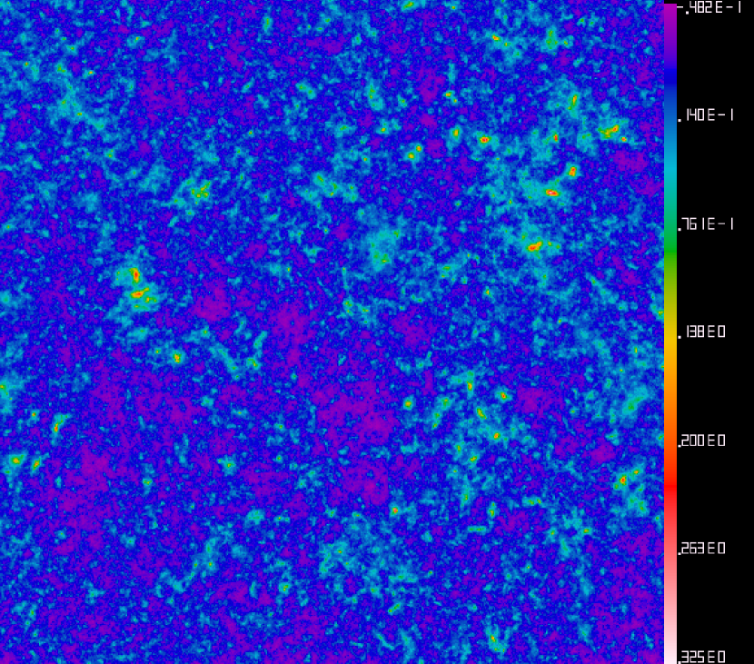
Figure 2: A $\kappa$ map in the N-body simulation of a $\Omega_{0}=0.4$ $\Lambda$CDM cosmology. The map width is 3.18 degree and has $2048^{2}$ pixels. The scale is in units of $\kappa$. The skewness of the distribution is apparent. Decreasing the cosmological density while maintaining the same variance forces structures to become more linear, and thus more skewed.

From the sectional maps, we also produce shear maps. These $\gamma$ maps are used to produce mock galaxy catalogs to check the data analysis pipeline and to calibrate the results. For each sectional $\kappa$ maps, we computed sectional $\gamma_{1}$ and $\gamma_{2}$ maps using FFT’s. The periodic boundary conditions on each section allow us to circumvent the boundary condition issue. Then by the same projection procedure, we make $40$ $\gamma_{1}$ and $\gamma_{2}$ maps with the same fields of view. We sample these simulated shear maps at the actual galaxy position from the Virmos-Descart catalog, which ensures that the mock catalogs have same masks and weights. Since the Virmos-Descart catalog consists of four fields, we can make ten full sets of mock catalogs from each simulation.

With these maps, we simulate the Virmos-Descart survey. Our goal is to measure $S_{3}$ of smoothed $\kappa$ fields and its dispersion and distribution in simulated survey catalogs to provide calibrations for the data analysis. In this paper, we fix the smoothing function as the compensated Gaussian function with a filter radius $\theta_{f}=5.374$ arc min. The maps we obtained above are non-periodic after the projection. In order to eliminate the edge effect, we cut $10\%$ from the four margins of each smoothed $\kappa$ map. For the noise-free maps, the $S_{3}$ parameter is defined as

$$S_{3}(\theta_{f})=\frac{\langle{\bar{\kappa}}^{3}\rangle}{\langle{\bar{\kappa}}^{2}\rangle^{2}}.$$ (4)

We used the $\kappa$ maps to fit the dependencies of $S_{3}$ on $\Omega_{0}$. We parametrized the relation as

$$S_{3}=\alpha\Omega_{0}^{-\beta}.$$ (5)

The best fit values for $\alpha$ and $\beta$ are

$$\alpha=66.0\pm 2.3,\ \ \ \ \beta=-0.64\pm 0.03,$$ (6)

which are similar to those obtained from second order perturbation theory with different window functions.

4 Analysis

4.1 Optimality

The optimal estimation of power spectra for Gaussian random fields is well understood. It requires a weighting of the data by the inverse of signal plus noise correlators. This procedure generally costs of order $O(N^{3})$ where $N$ is the number of data points, about one million for our catalog where we have two observables, $\gamma_{1},\gamma_{2}$ per galaxy. Clearly the optimal procedure is prohibitively expensive. In principle rapid multi-scale iterative algorithms allow an analysis in $O(N)$ (Padmanabhan et al., 2002). The cost prefactor in that algorithm is still large, and we decided to use the two point correlation function instead, whose computational cost is $O(N\log N)$ with a small prefactor.

Computing the two point correlation function is in general not an optimal estimator of the power. Being a quadratic estimator, it weights each data bin by only its local noise. Each correlation function bin $q_{i}$ is an inverse noise $N^{-1}$ weighted estimator of the data $\Delta$ for a bilinear form $Q_{i}$:

$$q^{i}=\Delta^{T}N^{-1}Q_{i}N^{-1}\Delta$$ (7)

while an optimal estimator should have used $(S+N)^{-1}$ as its weights instead. In the limit that signal to noise is small, the correlation function is optimal, similarly it is optimal if the signal and noise covariance matrices commute. For weak lensing surveys, on small scales signal to noise is small, while on larger scales the coverage is reasonably uniform, so a correlation function is not a very poor estimator.

To discuss the accuracy of the higher moments of a slightly non-Gaussian random field, consider the one point statistic of a filtered convergence field. The intrinsic distribution of ${\bar{\kappa}}$ is described by $P_{\kappa}$. We observe a noisy realization thereof, ${\bar{\kappa}}^{o}={\bar{\kappa}}+\nu$, with $\nu$ denotes a noise random variable. Its variance is $\sigma_{o}^{2}=\sigma_{\bar{\kappa}}^{2}+\sigma_{\nu}^{2}$. Typically the variance is noise dominated, in which limit the fractional accuracy of measuring $\sigma_{\bar{\kappa}}^{2}$ when $\sigma_{\nu}^{2}$ is known is

$$\frac{\Delta\sigma_{\bar{\kappa}}^{2}}{\sigma_{\bar{\kappa}}^{2}}=\sqrt{\frac{2}{n}}\frac{\sigma^{2}_{\nu}}{\sigma^{2}_{\bar{\kappa}}}$$ (8)

where $n$ is the number of independent samples. On the scales of a few arc minutes where this is best measured, signal to noise is below unity, and an accurate measurement is done statistically where one can reduce the noise due to the large number of arc minute sized patches in the survey.

The skewness is even harder to measure. One expects

$$\frac{\Delta{\bar{\kappa}}^{3}}{{\bar{\kappa}}^{3}}=\sqrt{\frac{15}{n}}\left(\frac{\sigma_{\nu}}{\sigma_{\bar{\kappa}}}\right)^{3}\frac{1}{S_{3}\sigma_{\bar{\kappa}}}$$ (9)

The last term is of order unity. Comparing with (8) we notice three losses: 1. The numerical prefactor increases. 2. The error scales as a higher power of signal to noise. 3. The denominator has increased powers of the converge variance, which is itself a small number. These trends suggest that higher moments are increasingly difficult to measure in noisy data.

Optimality of measuring the three point function is a challenging problem. Gaussian fields have zero three point function, so its distribution is intrinsically non-linear and must be measured either through high order perturbation theory or in simulations. By optimality of an estimator we mean one which minimizes the variance. The variance of the three point function is related to the six point function, which is a complex problem.

We thus scale back our ambitions, and concentrate on the skewness in a smoothed density field. In analogy with the two point function, we expect that an inverse noise squared weighting should be a reasonable procedure in this noise dominated measurement.

4.2 Two point functions

We first review the efficient computation of two point functions as a warm up exercise for the three point. Computationally, we start with the two shear estimates for each galaxy, and its noise estimate. The weight for each galaxy is the inverse noise variance. The noise variance is the quadratic sum of the intrinsic ellipticity variance $\sigma_{i}$, and the noise variance due to the PSF correction $\sigma_{e}$. The computation of $\sigma_{e}$ is described in Van Waerbeke et al. (2002): the galaxy catalogue is divided into cells of 30 galaxies each in the size-magnitude space. For each cell, the r.m.s. of the ellipticity correction gives an estimate of $\sigma_{e}$. We arbitrarily put a lower bound of 0.28 for the effective noise of any galaxy, as we do not want to give too large a weight to any individual object. Varying this cutoff does not seem to have significant effects on the results. The resulting weight per galaxy is therefore:

$$w_{i}={1\over{\rm max}(0.28,\sigma_{e})^{2}}.$$ (10)

Galaxies are mapped onto a grid using the cloud-in-cell algorithm (Hockney & Eastwood, 1988). The same is done for the weights. We now have three gridded quantities, which we fast Fourier transform. The autocorrelation of the weights is the inverse Fourier transform of the weight grid times its complex conjugate. Similarly, we obtain the two autocorrelations of the shear components, and two cross correlations, we denote them $\tilde{\xi}_{ij}$. If the dimensions of the grid are a factor of two larger than the spatial extent of the galaxies, the convolution on the grid does not introduce spurious boundary conditions.

The correlation functions are then multiplied by the angular weights, to yield two raw angular averaged correlation functions

$$\tilde{\xi}_{+}(r) = \frac{1}{2\pi}\int[\xi_{11}(r,\theta)+\xi_{22}(r,\theta)]d\theta$$

$$\tilde{\xi}_{-}(r) = \frac{1}{2\pi}\int[\xi_{11}(r,\theta)-\xi_{22}(r,\theta)]\cos(4\theta)+[\xi_{12}(r,\theta)+\xi_{21}(r,\theta)]\sin(4\theta)d\theta$$ (11)

and an angular averaged weight correlation $\tilde{\xi}_{w}$. The final correlation is then

$$\xi_{\pm}=\frac{\tilde{\xi}_{\pm}}{\tilde{\xi}_{w}}.$$ (12)

This allows a rapid computation of the two point function in eight Fourier transforms, each costing $2.5N\log_{2}(N)$ operations, where $N=4n_{x}n_{y}$ are the dimensions of the discretized grid, and the factor of 4 comes from having to use a Fourier grid of double the size to deal with the non-periodic boundary conditions. On a PC with the optimized Intel IPP or MKL libraries, the machines can sustain over a gigaflop on a 2 Ghz processor, so using even very fine grids $n_{x}\sim 10,000$ takes a matter of seconds.

The variance of the noise is uncorrelated between bins of the two point correlation function. One can see that the covariance of the two point function is a four point function. For a Gaussian field, that can be expanded in terms of two point functions. When the noise is white, a four point function only expands into a non-zero quantity when the four points have two coincident pairs. This is not possible when cross correlating two different correlation lags, and the covariance is thus zero. The error due to noise in each bin of the correlation function is $4/\tilde{\xi}_{w}$.

In tensor notation, the two point function can be written as a product of functions which depend on the magnitude of separation $r$, and angles of the unit separation vector $\hat{{\rm\bf x}}$

$$\xi_{abcd}({\rm\bf x}) \equiv \langle\gamma_{ab}(0)\gamma_{cd}({\rm\bf x})\rangle$$ (13)

$$= \frac{\xi_{+}(r)-\xi_{-}(r)}{2}(\delta_{ac}\delta_{bd}+\delta_{ad}\delta_{bc}-\delta_{ab}\delta_{cd})+4\xi_{-}(r)\left(\hat{x}_{a}\hat{x}_{b}-\frac{\delta_{ab}}{2}\right)\left(\hat{x}_{c}\hat{x}_{d}-\frac{\delta_{cd}}{2}\right)$$

4.3 Three point functions

The three point function is computationally more complex. We describe here the algorithm we implemented which computes it in $O(N^{2}\log N)$ operations for $N$ galaxies. We first describe the mathematical enumeration of the three point function which is prohibitively expensive. We then describe a faster procedure which computes the same quantity in a shorter time.

At every point we measure two components of the shear. The shear three point function has eight components. To reduce the complexity of the problem, we express the components of the shear in the coordinate system of the line connecting the first two points. We define the first point to be at the origin, and the second point along the x-axis at some distance $r$. The third point can be anywhere in the upper half plane. For each galaxy, we first label it point 1. We search rightward, and consider the set of all pairs formed from point 1 and a rightward neighbor, which we successively label as point 2. For each pair 1-2, we consider all galaxies with x coordinates larger than that of galaxy 1, and y coordinates above the line connecting point 1 to point 2. This results in a unique counting of triangles. As for the two point function, we multiply the shear estimates by the weight. We then compute the raw three point functions for the weighted shear, as well as for the weights. The final three point function is the quotient of the two.

At face value this would appear to be an $O(N^{3})$ operation, which is prohibitively expensive for $\sim 10^{5}$ galaxies which we currently have in each field. Analogous to particle-mesh simulations, we map all galaxies onto a two dimensional grid using a chaining mesh. This results in a linked list of galaxies residing in each cell, and costs $O(N)$ operations to construct. This allows us to find galaxies within some locus without searching the whole list.

We enumerate all pairs of galaxies. Each pair has a separation and an angle of the line connecting them relative to the x-axis. We grid the list of all pairs onto a four dimensional grid labeled by the position of the first galaxy, and their separations and angles. The grid of separations are chosen logarithmically. The angles run in the range $(-\pi/2,\pi/2)$, since we only need to count each pair once. For each separation and angle, we convolve this list of pairs with the gridded field of galaxies. We accumulate the three point function by averaging over the angles. In this process, we use only the pair-singlet cross correlation at lags with $\Delta x>0$ and $y$ values above the line describing the first pair. This way all triangles are counted exactly once.

In practice, gridding a Virmos-Descart field with 100,000 galaxies on $512^{2}$ cells, using 40 logarithmic separations and 20 angles takes about 15 minutes on the CITA GS320 alpha server which has 32 alpha processors running at 731 Mhz. The procedure requires 15GB of memory to store the four dimensional list of pairs.

The final three point function is defined on a three dimensional grid. In the intermediate pair enumeration we used polar coordinates to save storage and reduce computational cost. Since each pair is tagged by the coordinate of the left galaxy, the three point function has some angular smearing (in our case 9 degrees), so that large relative errors can accrue when galaxies 2 and 3 are nearby to each other but far from galaxy 1. This can be overcome by mapping $x$ to $-x$ and repeating the procedure. For the windowed skewnesses these skinny triangles do not contribute much, and we neglect this effect. In principle one could construct a three point function in $O(N\log(N))$ using a tree algorithm. The challenge is that the opening angle has to be chosen small since the shear needs to be rotated by the mean angle.

4.4 Skewness

We review the integration of the third moment from the three point function. A smoothed $\kappa$ map is defined as

$${\bar{\kappa}}({\rm\bf x})=\int\kappa({\rm\bf x}^{\prime}){\cal U}(|{\rm\bf x}-{\rm\bf x}^{\prime}|)d^{2}x^{\prime}$$ (14)

so the third moment can be expressed in terms of an integral over the three point function

$$\langle{\bar{\kappa}}^{3}({\rm\bf x})\rangle = \frac{1}{A}\int\kappa({\rm\bf x}^{\prime})\kappa({\rm\bf x}^{\prime\prime})\kappa({\rm\bf x}^{\prime\prime\prime}){\cal U}(|{\rm\bf x}-{\rm\bf x}^{\prime}|){\cal U}(|{\rm\bf x}-{\rm\bf x}^{\prime\prime}|){\cal U}(|{\rm\bf x}-{\rm\bf x}^{\prime\prime\prime}|)d^{2}xd^{2}x^{\prime}d^{2}x^{\prime\prime}d^{2}x^{\prime\prime\prime}$$ (15)

$$= 2\pi\int\xi_{3}(r,{\rm\bf x})U_{3}(r,{\rm\bf x})rdrd^{2}x$$ (16)

where $A$ is the area of integration. The three point function $\xi_{3}$ is defined with the first point at the origin, the second along the x axis, and the third anywhere in the plane. The window $U_{3}$ is the overlap integral of three filter functions placed at the same three locations. Due to symmetry, it is sufficient to consider only the upper half of the plane.

The integrands can be evaluated analytically for a compensated Gaussian filter (Crittenden et al., 2002). We choose

$${\cal U}=\frac{1}{2\pi r_{0}^{2}}\left(1-\frac{r^{2}}{2r_{0}^{2}}\right)\exp\left(\frac{-r^{2}}{2r_{0}^{2}}+1\right).$$ (17)

This filter has zero area, and is normalized to have a peak amplitude of unity in Fourier space. This has the feature that the filter will only damp modes, and never amplify. Its Fourier transform is ${\cal U}(k)=(kr_{0})^{2}\exp(-k^{2}r_{0}^{2}/2+1)/2$. The filter peaks at wave number $k_{0}=\sqrt{2}/r_{0}$. When $r_{0}$ is measured in radians, $k$ is the spherical harmonic number $l$. When integrated over a flat spectrum with constant $l^{2}C_{l}$, the area in Fourier space is $e^{2}/8$. One can use this window as a reasonable broad band Fourier power estimator. One obtains the equivalent flat power by multiplying the variance by $8/e^{2}$. The effective full width at half max width of the filter in Fourier space is a multiplicative factor of 2.34.

The corresponding shear filter is

$${\cal Q}={\cal U}-\frac{2}{r^{2}}\int_{0}^{r}r^{\prime}{\cal U}(r^{\prime})dr^{\prime}=-\frac{r^{2}}{4\pi r_{0}^{4}}\exp\left(\frac{-r^{2}}{2r_{0}^{2}}+1\right)$$ (18)

The filtered convergence field is then

$${\bar{\kappa}}({\rm\bf x})=\int\gamma_{ij}({\rm\bf x}^{\prime}){\cal Q}(|{\rm\bf x}-{\rm\bf x}^{\prime}|)\Delta\hat{x}_{i}\Delta\hat{x}_{j}d^{2}x^{\prime}.$$ (19)

Due to the $r^{2}$ term in front of ${\cal Q}$, the hatted objects in the integral are polynomials, and the integrand contains only Gaussian integrals over polynomials, which are exactly solvable. The smoothed variance can be derived in terms of the tensor shear correlation (13)

$$\langle{\bar{\kappa}}_{E}^{2}\rangle=\int\xi_{abcd}({\rm\bf x})W_{abcd}({\rm\bf x})d^{2}x$$ (20)

for the window function

$$W_{abcd}({\rm\bf x}) = \frac{1}{4(2\pi)^{2}r_{0}^{4}}\int x^{\prime}_{a}x^{\prime}_{b}(x^{\prime}_{c}-x_{c})(x^{\prime}_{d}-x_{d})\exp\left[-\frac{x^{\prime 2}+(x^{\prime}-x)^{2}}{2r_{0}^{2}}+2\right]d^{2}x^{\prime}$$ (21)

$$= \frac{4(\delta_{ac}\delta_{bd}+\delta_{ad}\delta_{bc})r_{0}^{4}-2(\delta_{ac}x_{b}x_{d}+\delta_{ad}x_{b}x_{c}+\delta_{bc}x_{a}x_{d}+\delta_{bd}x_{a}x_{c})r_{0}^{2}+x_{a}x_{b}x_{c}x_{d}}{2^{8}r_{0}^{4}\pi}$$

$$\times\exp\left(-\frac{x^{2}}{4r_{0}^{2}}+2\right)$$

where we have dropped all trace terms which do not contribute.

For the skewness we can similarly write

$$\langle{\bar{\kappa}}^{3}\rangle=2\pi\int\xi_{abcdef}(r,{\rm\bf x})W_{abcdef}(r,{\rm\bf x})rdrd^{2}x$$ (22)

where the corresponding window function $W_{abcdef}$ is an integral described below.

Since the filter (17) is the Laplacian of a Gaussian, convolving by it is equivalent to first taking the Laplacian of the $\kappa$ field, and convolving that by a Gaussian. The Laplacian of the $\kappa$ field is also a local second derivative of the shear field, for which a purely local decomposition of the shear field into $E$ and $B$ mode results independent of survey geometry. We thus expect minimal coupling between $E$ and $B$ modes from survey geometry.

To construct the analogue for the three point function, it is convenient to define the vectors which point from each vertex to the sum of the other two vertex vectors $q=x^{\prime}+x^{\prime\prime}$, $q^{\prime}=x^{\prime\prime}-2x^{\prime}$ and $q^{\prime\prime}=x^{\prime}-2x^{\prime\prime}$. They are depicted geometrically in Figure 3.

Figure 3: three point configuration: we place one vertex of the triangle at the origin, the second along the x axis, and the third in the upper half plane. The $q$ vectors are the axes along which each shear component needs to be projected.

The non-vanishing terms in the integral are

$$W_{abcdef} = \frac{e^{3}}{(2\pi)^{2}2^{3}3^{7}r_{0}^{10}}\left[q_{a}q_{b}q^{\prime}_{c}q^{\prime}_{d}q^{\prime\prime}_{e}q^{\prime\prime}_{f}\right.$$ (23)

$$+3\times 4\delta_{ac}q_{b}q^{\prime}_{d}q^{\prime\prime}_{e}q^{\prime\prime}_{f}+({\rm 3\ cyclic\ permutations})$$

$$+9(\delta_{ac}\delta_{be}+\delta_{ae}\delta_{bc})q^{\prime}_{d}q^{\prime\prime}_{f}+({\rm 12\ permutations})$$

$$\left.+9\times 2(\delta_{ac}\delta_{bd}+\delta_{ad}\delta_{bc})q^{\prime\prime}_{e}q^{\prime\prime}_{f}+({\rm 3\ cyclic\ permutations})\right]$$

$$\times\exp\left[-\frac{x^{\prime 2}+x^{\prime\prime 2}+(x^{\prime\prime}-x^{\prime})^{2}}{6}\right]$$

To check for systematics, one can compute the moments of the $B$ mode skewness $\langle{\bar{\kappa}}_{B}^{3}\rangle$ by a 45 degree rotation, corresponding to $(\gamma_{1},\gamma_{2})\longrightarrow(\gamma_{2},-\gamma_{1})$. Similarly one can get the moments $\langle{\bar{\kappa}}_{E}{\bar{\kappa}}_{B}^{2}\rangle$ and $\langle{\bar{\kappa}}_{E}^{2}{\bar{\kappa}}_{B}\rangle$. When we substitute the three point window (23) into three point integral (16), we place ${\rm\bf x}^{\prime}$ along the x-axis, requiring only a one-dimensional integral, and only integrate ${\rm\bf x}^{\prime\prime}$ on the upper half of the plane, since we only count each triangle once. The sum over the 6 indeces only has 8 independent components, corresponding to the two shear components at each of the three vertices.

In analogy to the two point function, we can compute the expected noise variance in each windowed skewness. The covariance between bins is again zero for white noise, since the only non-trivial six point function consists of three pairs. As for the two point function, we measure the noise from the variance between bins in the three point function, and assume that the noise is linearly proportional to the inverse square root. We verified the procedure by sampling four of the simulated images in the $\Omega_{0}=0.2$ simulation on a regular $400^{2}$ grid with equal weights, and computing the skewness from the three point function. For these 2.86 degree images this skewness agreed with the image skewness to better than ten percent on the 5.37 arc minute scale, which is consistent with the variation expected from the different weighting of the boundary.

5 Results

We show the measured skewness in Figure 4. The variance in the same filter from the two point function is shown in Figure 5. We find that statistical errors from galaxy noise are small, but on all scales we see some $B$ mode. The $B$ mode is more significant in the variance measurement than in the skewness. This is to be expected, since variances are always positive, while skewness may cancel.

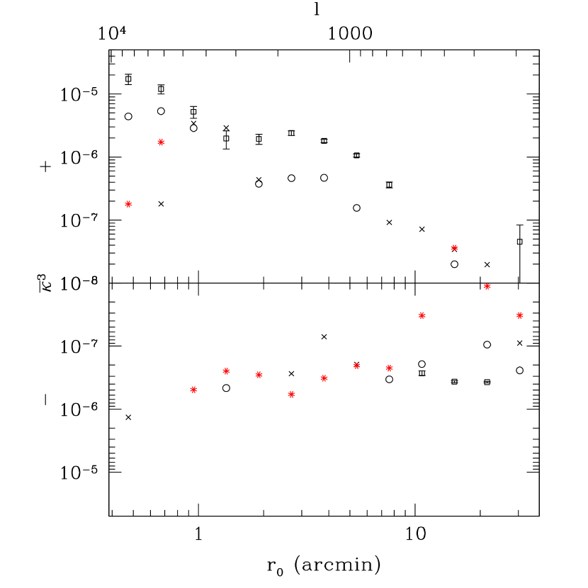
Figure 4: Skewness of the shear field. The lower panel shows the negative values for any variable which goes below zero. The boxes with error bars are the $E$ mode. The stars are the $B$ mode, the circles are $EB^{2}$ and the crosses are $E^{2}B$. The error bars reflect the scatter expected in the absence of a signal, and does not include signal sample variance.

Figure 5: Variance of the shear field. The right side label is offset by a factor of $8/e^{2}$ which gives the conversion to flat bandpower. The boxes are the lensing $E$ mode minus the non-lensing $B$ mode, while the crosses are the non-lensing $B$ mode. The error bars include the statistical error from shot noise plus the amplitude of $B$. The solid curve is the log-linear Fourier space window function used for the current analysis, which corresponds to a scale of 5.37 arc minutes. The vertical dotted line marks this scale. The dashed curve is the ensemble average obtained from 40 simulated maps in the $\Omega_{0}=0.4$ model.

After having obtained these statistics, we were primarily concerned by systematic errors, of which the $B$ mode is a potential diagnostic. In our arbitrary binning, the scale at 5.37 arc minutes had the smallest $B$ mode in the variance, so we proceeded with all further analyses using this scale. At this scale we find ${\bar{\kappa}}^{3}=1.06\pm 0.06\times 10^{-6}$. These errors are Gaussian and contain only contributions from noise. Similarly, we find a variance at the same scale of ${\bar{\kappa}}^{2}=6.30\pm 0.62\times 10^{-5}$. To model the possible effects of the $B$ mode, we added the observed $B$ power to the error bar, and subtracted the measured $B$ power from the signal. Our adopted value for subsequent analysis is ${\bar{\kappa}}^{2}=5.32\pm 0.62\pm 0.98\times 10^{-5}$, where second error bar is the magnitude of the $B$ mode.

The B-mode may or may not contribute to the skewness, which depends on the parity of the source of B modes. The measured value is consistent with zero, so we neglect it in the skewness interpretation. Since variances are always positive, one expects any spurious source of systematics to increase the observed variance. Any corrections due to a observed $B$ mode would also correct the observed signal down. For the skewness, the effect could have either sign. We therefore did not correct the $\langle\bar{\kappa}^{3}\rangle$ values.

Using the skewness and variances we can construct $S_{3}$. The actual value of the $B$ variance is added to to the error bar of the variance. The noise errors are Gaussian since they arise from the mean of a very large number of data points. In the absence of a better model, we also treat the systematic error as Gaussian. The resulting $S_{3}$ is shown in Figure 6. Random variables which are quotients of Gaussians, such as $S_{3}$, don’t generally have well defined moments. The error bars in the plot are obtained by taking one sigma on each of $\langle{\bar{\kappa}}^{3}\rangle$ and $\langle{\bar{\kappa}}^{2}\rangle$, and plotting the observed change in $S_{3}$. For sums of Gaussians this is like summing the standard deviations, which is always an overestimate of the actual standard deviation of the sum. One can consider the error bars in figure 6 to be a conservative estimate. For our scale of 5.37 arc minutes, we used a second error metric by Monte-Carlo sampling of Gaussian noise. Nominally, $S_{3}=375$, and the Monte-Carlo sample finds the median and percentile spreads are $S_{3}=376^{+242}_{-125}$ at $68\%$ confidence, and $S_{3}=376^{+815}_{-194}$ at $95\%$. Again, these error bars do not include sample variance, which depends on cosmological models and require N-body simulations to calibrate.

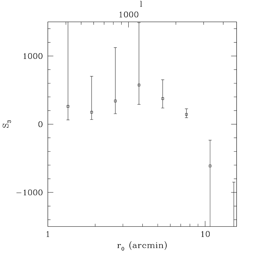
Figure 6: $S_{3}$ for the data, where we used $E^{2}-B^{2}$ as the estimator for ${\bar{\kappa}}^{2}$. We added the amplitude of the $B$ mode to the error bar, which is described in the text.

In principle, the fit (5) gives us a value of $\Omega_{0}$, which would be a very small value, indicating that the data prefers a low density universe with no practical lower bound. The error bar and confidence interval is a tricky task, since it requires knowledge of the area and geometry of the sky patch surveyed. In principle, it should scale as the inverse square root of the number of independent patches as given by Equation (9). At the scales of the filter size of 5.37 arc minutes the survey is quite irregular, and it is not easy to quantify the effective area of sky observed, nor the correlation between patches. So to measure the scatter we use the noise-free mock catalogs from simulations. We process these catalogs through the same three point function simulation pipeline. Even though the simulated catalogs have no noise, we used the same weights as the noisy data. This allows us to separate the error from sample variance from the error from noise.

In figures 7 and 8 we show the results for a $\Omega_{0}=0.4$ model obtained through the pipeline. The points are the average from ten mock catalogs, and the error bars are the standard deviation across the ten catalogs. The mode separation for the variances is typically better than 1%, while skewness estimates have crosstalk at the 10% level. The plots also include the ensemble averages from the 40 direct idealized ${\bar{\kappa}}$ maps, processed through an independent analysis which shares only the N-body simulation output, which is a useful cross-check of the pipeline. The fit from Peacock & Dodds (1996) is also plotted as the dotted line, which provides a second reference for the resolution of the simulation. We note good agreement for scales larger than 1 arc minute, but below which the simulations are limited by resolution.

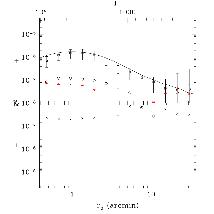
Figure 7: Skewness in a noise free $\Omega_{0}=0.4$ simulation processed through ten mock catalogs and the entire pipeline. Actual galaxy positions and weights were used. The symbols have the same meaning as in figure 4, with the points denoting the average over ten mock catalogs, and the error bar the standard deviation. The solid curve is the ensemble average from the $\kappa$ maps. The agreement is a cross check on the analysis pipeline. We note that the estimate of the standard deviation has an error of 47% with the 10 mock catalogues that were used.

Figure 8: Variances in the same simulation as figure 7. The mode separation works better for the variance than for the skewness, and the mock catalogs have significantly smaller sample variance on ${\bar{\kappa}}^{2}$ than for ${\bar{\kappa}}^{3}$. The solid curve is the same as the dashed line in figure 5, which is the ensemble average from the $\kappa$ maps. The dotted line is the fit from Peacock & Dodds (1996).

While the error bars in figures 4 and 5 only accounted for the noise, the simulation plots show only the sample variance. The sample variance is clearly decreasing at smaller scales, where more independent patches are used. At scales below one arc minute, the simulations are probably limited by resolution.

To estimate the sample variance errors, we used a sample of forty simulated galaxy catalogs. This number is limited by the expense of computations. The sample consisted of our four simulation models with ten catalogs for each model. We scaled the skewness and variance in each model by the inverse of the standard deviation of the same quantity obtained from the simulated maps. This set of normalized samples was used to Monte Carlo sample 10000 instances of ${\bar{\kappa}}^{3}$ and ${\bar{\kappa}}^{2}$. For a given trial value of $\Omega_{0}$, we fixed ${\bar{\kappa}}^{2}$ to the observed value, and used ${\bar{\kappa}}^{3}$ from Equation 5. The normalized samples are scaled to these constraints, and we randomly draw from the 40 simulated values. We add noise drawn from a Gaussian with the appropriate variance. This allows us to form a value for $S_{3}$ for each sample. We find the confidence bounds using a uniform Bayesian prior. For $\Omega_{0}=0.25$ we found 20% of the samples to have $S_{3}$ larger than the observed value, while for $\Omega_{0}=0.5$ only 10% of the samples hasd $S_{3}$ larger than observed. For $\Omega_{0}=1$ such large values of $S_{3}$ were never found. We note that our limited simulation sample only provides a crude estimate of the errors. It is probably not meaningful to derive 95% statistics from this small sample whose wings are non-Gaussian. The preliminary interpretation is that a low value of $\Omega_{0}$ is favored. More detailed systematic numerical studies are in progress. No practical lower bound on $\Omega_{0}$ is derived, since below $\Omega_{0}=0.2$ the empirical fit from Equation (5) has not been calibrated.

We compared the sample variance in the simulated maps to that of the mock catalogs. For the scale of interest, we found the scatter in ${\bar{\kappa}}^{2}$ from the mock catalogs shown in figure 8 consistent with that of a 8.5 sq degree ${\bar{\kappa}}$ map, which is the effective area sampled by our survey. The scatter in ${\bar{\kappa}}^{3}$ from the mock catalogs was significantly larger than in a 8.5 sq degree contiguous map, possibly closer to what one sees across 3 sq degree maps. This suggests that the inverse noise variance weights are not optimal to estimate skewness. Unfortunately with the limited number of mock catalogs, the error on the sample variance is large, and more simulations are needed. To test the resolution of the simulations, we also compared the results for a simulation with half as many particles in directions on a grid twice as coarse. In the $\Omega_{0}=0.3$ model, the resulting $S_{3}$ on the ${\bar{\kappa}}$ maps changed by less than one percent. The variance and skewness separately changed by about 10% and 20% respectively, and one would expect the changes to be significantly smaller compared to a higher resolution simulatio. We thus expect that simulation resolution should not be a major source of error on these scales.

We also examined the variance between the four Virmos-Descart fields. At the scale of 5.37 arc minutes, the fields F14, F02, F22 and F10 had ${\bar{\kappa}}^{3}$ of $8.7\times 10^{-8},1.1\times 10^{-6},-5.1\times 10^{-7},1.1\times 10^{-6}$ respectively. Their individual values of ${\bar{\kappa}}^{2}$ were $3.0\times 10^{-5},7.0\times 10^{-5},7.5\times 10^{-5},7.0\times 10^{-5}$ without any subtraction of a $B$ mode. This scatter is consistent with that seen in the mock catalogs. One could in principle use the observed scatter to model the sample variance, but with only four fields, the error in the scatter is $\sqrt{2/3}$ which is very large, so we used the larger sample of simulated mock catalogs.

Several other factors also affect the skewness interpretation. Source-Lens-Clustering (Hamana et al., 2002a; Bernardeau, 1998) for example systematically reduces the observed skewness, which would strengthen the inferred bounds on $\Omega_{0}$. Using Table 3 from Hamana et al. (2002a), the closest model to our data is probably C1, which for a non-evolving source distribution and the closest comparable window size of 10 arc minutes results in a 16% effect.

The current analysis is limited by sample variance, which will improve dramatically with the CFHT legacy survey. The error on the error estimate is not yet well determined, requiring more simulations to quantify. Errors in the source redshift distribution also effect the results. These effects are expected to be small compared to the sample variance. Work on this issue is in progress, and we expect an order of magnitude improvement in the near future. The precise numerical computation of skewness is also a challenge, as different groups measure slightly different normalizations for the variance (White & Hu, 2000; Jain et al., 2000). For the current data, the differences are not substantial, but need to be tightened with larger and more accurate galaxy catalogs. Currently only one angular scale was used, which is one with the smallest $B$ mode contamination in the variance measurement. Even on this optimal scale, the $B$ mode will soon become a limiting factor when the survey area is increased.

6 Conclusions

We have presented the first direct measurement of dark matter skewness using weak gravitational lensing in the Virmos-Descart survey. We chose the compensated Gaussian with a scale of 5.37 arc minutes for all analyses, which had the smallest $B$ mode, consistent with zero. At this scale, the skewness of the dark matter is ${\bar{\kappa}}^{3}=1.06\pm 0.06\times 10^{-6}$. We measured the variance ${\bar{\kappa}}^{2}=5.32\pm 0.62\pm 0.98\times 10^{-5}$.

This implies $S_{3}=375^{+342}_{-124}$. Calibrating to mock catalogs from N-body simulations, we find $\Omega_{0}<0.5$ at 90% and $\Omega_{0}<0.25$ at 80% confidence. The errors are dominated by sample variance. The CFHT legacy survey will increase the sky area by a factor of 20, which should result in a decrease of a factor of 4 in the error in a year’s time. Better constraints could also be obtained by going to smaller scales, where sample variance is smaller. This requires higher resolution simulations, faster three point analysis, and a better understanding of the origin of the $B$ mode.

This work was supported in part by the TMR Network “Gravitational Lensing: New Constraints on Cosmology and the Distribution of Dark Matter” of the EC under contract No. ERBFMRX-CT97-0172, the Canada Foundation for Innovation funded computing infrastructure, and NSERC grant 72013704. We thank Francis Bernardeau, Peter Schneider for very interesting and long discussions on skewness and other 3-pt estimators. We thank Uros Seljak for the dark matter projection code, and Mike Jarvis for correction equation (21). TJZ would like to thank CITA for its hospitality during his visit.

References

- Bacon et al. (2002) Bacon, D., Massey, R., Refregier, A., & Ellis, R. 2002, in eprint arXiv:astro-ph/0203134, 3134–+
- Bernardeau (1998) Bernardeau, F. 1998, A&A, 338, 375
- Bernardeau et al. (2002) Bernardeau, F., Mellier, Y., & van Waerbeke, L. 2002, A&A, 389, L28
- Bernardeau et al. (1997) Bernardeau, F., van Waerbeke, L., & Mellier, Y. 1997, A&A, 322, 1
- Bernardeau et al. (2003) —. 2003, A&A, 397, 405
- Brown et al. (2002) Brown, M. L., Taylor, A. N., Bacon, D. J., Gray, M. E., Dye, S., Meisenheimer, K., & Wolf, C. 2002, in eprint arXiv:astro-ph/0210213, 10213–+
- Crittenden et al. (2002) Crittenden, R. G., Natarajan, P., Pen, U., & Theuns, T. 2002, ApJ, 568, 20
- Davis & Peebles (1983) Davis, M. & Peebles, P. J. E. 1983, ApJ, 267, 465
- Hamana et al. (2002a) Hamana, T., Colombi, S. T., Thion, A., Devriendt, J. E. G. T., Mellier, Y., & Bernardeau, F. 2002a, MNRAS, 330, 365
- Hamana et al. (2002b) Hamana, T., Miyazaki, S., Shimasaku, K., Furusawa, H., Doi, M., Hamabe, M., Imi, K., Kimura, M., Komiyama, Y., Nakata, F., Okada, N., Okamura, S., Ouchi, M., Sekiguchi, M., Yagi, M., & Yasuda, N. 2002b, in eprint arXiv:astro-ph/0210450, 10450–+
- Hockney & Eastwood (1988) Hockney, R. W. & Eastwood, J. W. 1988, Computer simulation using particles (Bristol: Hilger, 1988)
- Hoekstra et al. (2002) Hoekstra, H., Yee, H. K. C., Gladders, M. D., Barrientos, L. F., Hall, P. B., & Infante, L. 2002, ApJ, 572, 55
- Jain et al. (2000) Jain, B., Seljak, U., & White, S. 2000, ApJ, 530, 547
- Jarvis et al. (2002) Jarvis, M., Bernstein, G., Jain, B., Fischer, P., Smith, D., Tyson, J. A., & Wittman, D. 2002, in eprint arXiv:astro-ph/0210604, 10604–+
- Kaiser (1987) Kaiser, N. 1987, MNRAS, 227, 1
- Padmanabhan et al. (2002) Padmanabhan, N., Seljak, U., & Pen, U. L. 2002, in eprint arXiv:astro-ph/0210478, 10478–+
- Peacock & Dodds (1996) Peacock, J. A. & Dodds, S. J. 1996, MNRAS, 280, L19
- Pen (1998) Pen, U. 1998, ApJ, 498, 60
- Pen et al. (2002) Pen, U., Van Waerbeke, L., & Mellier, Y. 2002, ApJ, 567, 31
- Refregier et al. (2002) Refregier, A., Rhodes, J., & Groth, E. J. 2002, ApJ, 572, L131
- Schneider & Lombardi (2002) Schneider, P. & Lombardi, M. 2002, in eprint arXiv:astro-ph/0207454, 7454–+
- Seljak & Zaldarriaga (1996) Seljak, U. & Zaldarriaga, M. 1996, ApJ, 469, 437+
- Takada & Jain (2002) Takada, M. & Jain, B. 2002, in eprint arXiv:astro-ph/0210261, 10261–+
- Van Waerbeke et al. (2000) Van Waerbeke, L., Mellier, Y., Erben, T., Cuillandre, J. C., Bernardeau, F., Maoli, R., Bertin, E., Mc Cracken, H. J., Le Fèvre, O., Fort, B., Dantel-Fort, M., Jain, B., & Schneider, P. 2000, A&A, 358, 30
- Van Waerbeke et al. (2002) Van Waerbeke, L., Mellier, Y., Pelló, R., Pen, U.-L., McCracken, H. J., & Jain, B. 2002, A&A, 393, 369
- Van Waerbeke et al. (2001) Van Waerbeke, L., Mellier, Y., Radovich, M., Bertin, E., Dantel-Fort, M., McCracken, H. J., Le Fèvre, O., Foucaud, S., Cuillandre, J.-C., Erben, T., Jain, B., Schneider, P., Bernardeau, F., & Fort, B. 2001, A&A, 374, 757
- White & Hu (2000) White, M. & Hu, W. 2000, ApJ, 537, 1
- Zaldarriaga & Scoccimarro (2002) Zaldarriaga, M. & Scoccimarro, R. 2002, in eprint arXiv:astro-ph/0208075, 8075–+