Ultraviolet spectroscopy of narrow coronal mass ejections

Abstract

We present Ultraviolet Coronagraph Spectrometer (UVCS) observations of 5 narrow coronal mass ejections (CMEs) that were among 15 narrow CMEs originally selected by Gilbert et al. (2001). Two events (1999 March 27, April 15) were “structured”, i.e. in white light data they exhibited well defined interior features, and three (1999 May 9, May 21, June 3) were “unstructured”, i.e. appeared featureless. In UVCS data the events were seen as $4-13^{\circ}$ wide enhancements of the strongest coronal lines H I Ly$\alpha$ and O VI $\lambda\lambda 1032,1037$. We derived electron densities for several of the events from the Large Angle Spectrometric Coronagraph (LASCO) C2 white light observations. They are comparable to or smaller than densities inferred for other CMEs. We modeled the observable properties of examples of the structured (1999 April 15) and unstructured (1999 May 9) narrow CMEs at different heights in the corona between $1.5~{}R_{\odot}$ and $2~{}R_{\odot}$. The derived electron temperatures, densities and outflow speeds are similar for those two types of ejections. They were compared with properties of polar coronal jets and other CMEs. We discuss different scenarios of narrow CME formation either as a jet formed by reconnection onto open field lines or CME ejected by expansion of closed field structures. Overall, we conclude that the existing observations do not definitively place the narrow CMEs into the jet or the CME picture, but the acceleration of the 1999 April 15 event resembles acceleration seen in many CMEs, rather than constant speeds or deceleration observed in jets.

1 Introduction

Coronal mass ejections (CMEs) are dynamic solar phenomena in which mass and magnetic field are ejected from the lower corona into the higher solar atmosphere and interplanetary space. They involve large scale changes to the coronal structure and reconfiguration of the coronal magnetic field. A commonly used definition of CMEs describes them as new, discrete, bright features appearing in the field of view of a white light coronagraph and moving outward over a period of minutes to hours (e.g. Munro et al., 1979). On the basis of this broad definition several classifications were introduced. The morphology and spectral characteristics of CMEs were extensively studied over the last decade (e.g. Hundhausen 1997; St. Cyr et al. 2000; Antonucci et al. 1997; Ciaravella et al. 1997, 2000, 2001). Apparent angular widths of the CMEs cover a wide range from few to 360 degrees (Howard et al. 1985; St. Cyr et al. 1999, 2000). The very narrow structures (narrower than about $15^{\circ}-20^{\circ}$) form only a small subset of all the observed CMEs and are usually referred to as rays, spikes, fans, etc. (Munro & Sime 1985; Howard et al. 1985).

Recently, Gilbert et al. (2001) conducted a study of 15 selected narrow CMEs observed in white light by the Large Angle Spectrometric Coronagraph (LASCO) aboard Solar and Heliospheric Observatory (SOHO) in the period from 1999 March through December. The selection criteria included the condition that the measurable angular width of the event is no more than $15^{\circ}$ and the CME is not part of a larger event. Moreover, the CMEs had to have a clear surface association in H$\alpha$ and/or He I data from the Mauna Loa Solar Observatory (MLSO), or in data from the Extreme Ultraviolet Imaging Telescope (EIT) on SOHO. Gilbert et al. (2001) examined the events’ structures, angular sizes and projected radial velocities within the LASCO C2 and C3 coronagraphs field of view ($2-32~{}R_{\odot}$), and likely surface associations. The narrow CMEs appeared to fall into two categories: “structured”, that exhibit well defined interior features in the LASCO images (7 events) and “unstructured”, that were featureless (8 events). In their exploratory study they did not find any obvious difference between narrow and large CMEs other than their appearance. The projected average radial velocities of the narrow CMEs ($\sim 400$ km s^-1) are similar to the average speed of the regular CMEs.

The solar corona manifests its activity in various ways. Besides CMEs, another type of eruptive event observed throughout the whole solar cycle is coronal jets. They are presumably triggered by field reconnection between a magnetic dipole and neighboring unipolar region (Wang et al. 1998). Different types of coronal jets were observed by various instruments: the Yohkoh Soft X–Ray Telescope (SXT) (Shibata et al. 1992) and SOHO Ultraviolet Coronagraph Spectrometer (UVCS), EIT, and LASCO (Moses et al. 1997, Gurman et al. 1998, Wang et al. 1998, Wood et al. 1999, Dobrzycka et al. 2000, 2002). The jets originate in a variety of settings; in UV and X-ray bright points within coronal holes, in active regions, flares, etc. In the white light coronagraphs they appear as narrow, fast and featureless, bright structures (Howard et al. 1985). They are often listed among CMEs as they satisfy the general CME definition.

According to the most popular models, coronal jets and CMEs are entirely different phenomena. A jet is taken to be the result of reconnection between open and closed field lines in which the gas may be strongly heated (X–ray jet), and it is accelerated by the magnetic tension force of the newly reconnected field lines (Shibata et al. 1992; Shimojo et al. 1996). CMEs, on the other hand, are attributed to the release of magnetic stress stored in a twisted flux rope (e.g. Amari et al. 2000; Gibson & Low 1998; Lin & Forbes 2000) or in a sheared arcade held down by overlying unsheared field (Antiochos, DeVore, & Klimchuk 1999).

In this project we study spectra of the narrow CMEs as they may shed some light on differences between narrow and large CMEs and, in particular, the relation of the narrow CMEs to coronal jets. We present ultraviolet spectroscopy of the several narrow CMEs that were originally selected by Gilbert et al. (2001). The data were obtained with the UVCS instrument on board SOHO. We describe the observations in § 2. In § 3 we discuss our results, model the observations, and compare narrow CMEs with coronal jets and other CMEs. Finally, we summarize the results in § 4.

2 Observations

The UVCS/SOHO instrument is designed to observe the extended solar corona from $1.4~{}R_{\odot}$ to about $10~{}R_{\odot}$ (Kohl et al. 1995). In 1999 the coronal spectra were acquired in the O VI spectrometer channel, which covers the wavelength ranges 940–1123 Å in first and 473–561 Å in second order. A mirror between the grating and the detector images spectral lines in the range 1160–1270 Å (580–635 Å in second order). The primary lines observed were H I Ly$\alpha$ $\lambda$1216 and O VI $\lambda\lambda$ 1032,1037.

To obtain spectra of the narrow CMEs we searched the UVCS archival data following the list of the LASCO events compiled by Gilbert et al. (2001). In 1999, each UVCS daily observing plan consisted of a 14 hour standard synoptic sequence and special observations designed by the lead observer. During the synoptic observations the slits were scanned radially at eight position angles (P.A.; measured counterclockwise from the north heliographic pole) $45^{\circ}$ apart at different heights ranging from $1.4~{}R_{\odot}$ up to $3.6~{}R_{\odot}$. UVCS had a chance to record the CME spectrum only when its pointing coincided with the event. This happened on five occasions out of fifteen listed by Gilbert et al. (2001). Most of the observations appeared as a part of the synoptic sequence. During the synoptic scans the instrument configuration included an entrance slit of 100 µm for the O VI channel corresponding to 28” or 0.4 Å. The spatial binning was 3 pixels (21”), and the grating position covered three spectral ranges: 1023.20–1043.75, 1208.72–1220.62 (with H I Ly$\alpha$ from the redundant mirror), 975.78–979.16 Å, with spectral binnings of 3, 2, and 2 pixels (0.298, 0.183, and 0.183 Å) respectively. The exposure time was $180-200$ s. Unfortunately, the synoptic program provides fairly short dwell times at each height, making it difficult to characterize time dependence of the events.

We obtained ultraviolet spectra of five narrow CMEs reported by Gilbert et al. (2001). The events on 1999 March 27 and April 15 were described as structured and events on 1999 May 9, 21, and 1999 June 3 as unstructured. Table 1 contains a summary of observations.

In the data reduction we followed the standard techniques described in Kohl et al. (1997, 1999). We used the latest version of the UVCS Data Analysis Software (DAS) (released in June 2001) for wavelength, intensity calibration, and removal of image distortion. The uncertainties in the line intensities are estimated to be $\pm 20\%$ and are due to photon–counting statistics, background subtraction, and radiometric calibration (Gardner et al. 2002). Table 2 lists measured profiles of the brightest emission lines, H I Ly$\alpha$, O VI $\lambda\lambda 1032,1037$ after the background corona (pre– or post–CME spectra, see below) was subtracted. In most cases (except very weak lines) to obtain the total intensities and $1/e$ widths we fitted multiple Gaussian functions to the observed profiles. A detailed description of this technique including the removal of the instrumental profile, background, stray light and interplanetary hydrogen contributions can be found in Kohl et al. (1997).

Following Gilbert et al. (2001) we attempted to identify the solar disk and/or lower corona associations of these events. We used data from EIT and SXT instruments. Also, most of the events were described in the daily reports by EIT and LASCO teams.

2.1 1999 March 27 (structured)

Gilbert et al. (2001) reported that this CME appeared in the LASCO C2 field of view at P.A$=310^{\circ}$, 16:54 UT and was $12^{\circ}$ wide. UVCS began a special CME watch campaign at 16:02 UT and continued it until 00:12 UT of the next day. The observations were centered at P.A.$=310^{\circ}$ and consisted of repeating sequences of eight exposures at $1.49~{}R_{\odot}$ and two at $1.85~{}R_{\odot}$. Each exposure was 75 s. The instrument configuration included an entrance slit of $50\micron$ and spatial binning of 3 pixels (21”). The grating and detector mask covered four spectral ranges: $1030.45-1039.16$, $997.53-1000.51$, $1212.14-1216.71$, $976.13-978.91$ Å, which allowed us to monitor the emission lines H I Ly$\alpha$, O VI $\lambda\lambda 1032,1037$, C III $\lambda 977$, Si XII $\lambda 499$ in second order, and others. The binning in the spectral direction was 2, 3, 1, and 2 pixels (0.199, 0.298, 0.092, 0.199 Å) in the four ranges, respectively.

The evidence for the CME passing the UVCS slit was seen from the beginning of observations at $1.49~{}R_{\odot}$. It appeared as an enhancement of the Ly$\alpha$ and O VI $\lambda\lambda 1032,1037$ line intensities in the spatial range between -100 and 250 arcsec, which corresponds to about $13^{\circ}$ of angular width. At 16:29 UT the slit was moved to $1.85~{}R_{\odot}$ for 3 minutes and the line intensity enhancement there was visible between -100 and 215 arcsec, which is consistent with $\sim 10^{\circ}$ of angular width. During the long coverage at $1.49~{}R_{\odot}$ both H I Ly$\alpha$ and O VI lines showed similar behavior. They reached maximum at 16:05–16:12 UT, then the intensity slightly decreased for about 10 minutes and increased again but did not reach the initial value. From about 17:25 UT the line intensities became consistent with the background.

We compared the CME observations with corresponding data obtained within the synoptic program on the same day but before the event. The radial scan centered at P.A.=315^∘ included observations at $1.49~{}R_{\odot}$ taken between 03:36 – 03:43 UT and observations at $1.85~{}R_{\odot}$ between 03:54 – 04:04 UT. We considered the correction for different pointing angle and verified that the same region in the pre–CME and CME data that was away from the CME remained unchanged. The emission line intensity variations away from the CME were within $10-15$% and $1/e$ widths were comparable at both heights. With respect to the pre–CME data the maximum H I Ly$\alpha$ intensity during the event was enhanced by $30-40$% at both heights, while the O VI lines showed increase by about 20% and close to 100% at $1.49~{}R_{\odot}$ and $1.85~{}R_{\odot}$ respectively. The measured line intensities with subtracted pre–CME profiles are summarized in Table 2. The O VI $\lambda 1032$ and O VI $\lambda 1037$ intensity ratio was 3 before the CME. During the ejection it dropped to about 2 at both heights due to the Doppler dimming effect (see § 3). The $1/e$ widths of the emission line profiles appeared comparable to the pre–CME values. In the post–CME spectra the lines were weaker than during the CME passage but still brighter than before the event. We did not detect any obvious Doppler shifts. Both C III and Si XII line intensities varied throughout the observations but the profiles were weak and could not be fitted. Also it was not clear if the variation was due to the CME.

On the disk, EIT data appeared to show the CME associated with a dark filament. It began to bubble between 12:00 and 15:36 UT and at 15:36 UT a dimming typical for CMEs was visible behind the limb. There were no SXT images available between 12:25 and 17:13 UT. After that the SXT data did not show any obvious association up to 18:43 UT. However, the next available image at 19:57 UT clearly displayed loops formed in that area.

2.2 1999 Apr 15 (structured)

This event was recorded by LASCO C2 at 07:54 UT, P.A.$=102^{\circ}$ and appeared to be $10^{\circ}$ wide. UVCS was taking a synoptic radial scan at P.A.$=90^{\circ}$ between 07:33 and 09:48 UT. The CME was detected at all heights: $1.38,1.50,1.62,1.74,1.98,2.33,2.88,$ and $3.62~{}R_{\odot}$. Brightening of the H I Ly$\alpha$ and both O VI $\lambda\lambda 1032,1037$ lines due to the CME was present at all exposures. However, during observations at $3.62~{}R_{\odot}$ the brightening was initially weak, becoming obvious only after several exposures, at about 09:31 UT. Then, the H I Ly$\alpha$ intensity increased by 35%. The O VI lines were too weak at this height and we were unable to fit the profiles. The bright feature in the CME spectra was centered at P.A.$=107-108^{\circ}$ and was $5-7^{\circ}$ wide. Figure 1 shows an example of spectral lines obtained at three different heights. The line profiles are blue shifted by about 50 km s^-1.

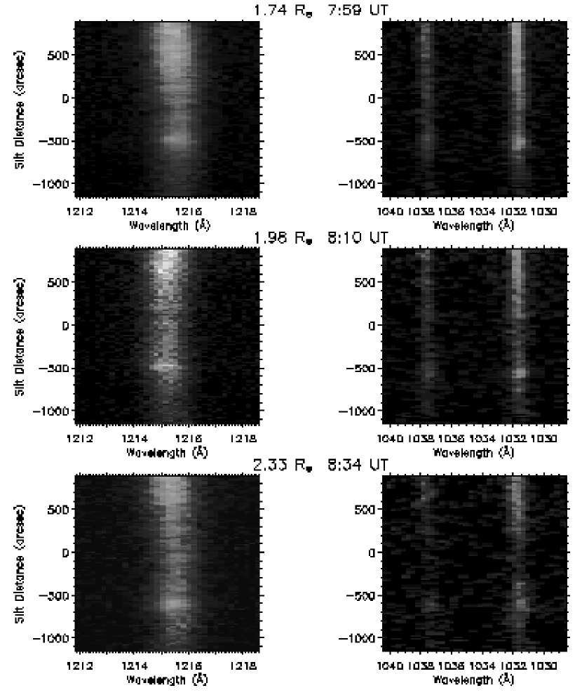
Figure 1: Examples of the UVCS observations of the 1999 April 15 narrow CME. The projected height and initial UT time of each exposure are shown. The vertical axis is the spatial coordinate along the UVCS entrance slit (in arcsec), centered at P.A.$=90^{\circ}$ at the indicated heliocentric distance. The CME appeared as a narrow brightening in the H I Ly$\alpha$ $\lambda 1216$ (left) and O VI $\lambda\lambda 1032,1037$ (right) emission lines at about $-600$ arcsec.

To compare the CME line profiles with the background corona we looked at the corresponding synoptic scan obtained a day earlier. However, it contained another transient structure visible at most heights and the line intensities were enhanced with respect to the background level. We found that the synoptic observations obtained 24 hours after the CME, on 1999 April 16, are more suitable for comparison. The line intensities, in the region of the corona away from the CME, were consistent with each other within $10-15$% and the $1/e$ widths were comparable at all heights. With respect to those data, H I Ly$\alpha$ line brightening due to CME ranged from 25% at 1.38 $R_{\odot}$ to about 50% at $1.98~{}R_{\odot}$, while the O VI lines were enhanced by $100-350$% at different heights. The O VI $\lambda\lambda 1032,1037$ line ratio was reduced from 2.8 to about $2-2.5$. The measured line intensities, after the post–CME profiles were subtracted, are summarized in Table 2.

Gilbert et al. (2001) noted that the EIT data point to association of this CME with a flare in the active region close to the East limb. In running difference EIT $\lambda 195$ images the activity appears to start between 05:36 and 06:00 UT with brightening and rising of several arcs inside the active region. By 08:12 UT the loop legs extend up reaching the edge of EIT field of view. There are no SXT images available for that period of time. In the LASCO daily report the event was described as a jet–like ejection.

2.3 1999 May 9 (unstructured)

This narrow CME appeared in LASCO C2 at 19:30 UT, P.A.=$100^{\circ}$ (Gilbert et al. 2001). It was recorded by UVCS in the extended synoptic observations at P.A.$=90^{\circ}$ between 19:17 and 20:53 UT. Brightening of the H I Ly$\alpha$ and O VI $\lambda 1032,1037$ lines centered at about P.A.$=100^{\circ}$ was visible at 1.38, 1.58, and $1.86~{}R_{\odot}$. The O VI lines showed enhancement also at $2.15~{}R_{\odot}$. We did not measure any significant Doppler shifts of the line profiles. The angular width of the CME was $4^{\circ}$.

To compare the CME line intensities with pre–CME profiles we used the corresponding synoptic data from the previous day, 1999, May 8. They were centered at the same position angle – P.A.$=90^{\circ}$, and covered heights from 1.38 to $3.62~{}R_{\odot}$ between 09:01 UT and 11:16 UT. We compared the emission line intensities in the region of corona away from the CME. The difference between line intensities on 1999, May 8 and May 9 was no more than $10-15$% and thus we accepted it as satisfactory agreement. The CME H I Ly$\alpha$ was $15-30$% and O VI $\lambda 1032,1037$ $20-50$% brighter with respect to the 1999, May 8 observations. The $1/e$ widths did not change significantly. The O VI line ratio decreased to 2.0 compared with the pre–CME value of about 3. Table 2 includes a summary of the measured line intensities after the pre–CME spectrum was subtracted.

Gilbert et al. (2001) noted that the CME was associated with an active prominence. It most likely originated from the back of the disk. The SXT image from 22:15 UT does not show any significant features that could be associated with the CME.

2.4 1999 May 21 (unstructured)

At the time of the CME passage UVCS was executing the synoptic program; the radial scan centered at P.A.$=270^{\circ}$ in particular. Gilbert et al. (2001) reported 02:06 UT as the time of appearance of the CME in the C2 field of view at P.A.$=290^{\circ}$. UVCS was observing at $3.62~{}R_{\odot}$ from 01:58 UT to 02:36 UT and recorded brightening of the O VI $\lambda 1032,1037$ lines beginning at 02:08 UT. The line brightening occurred close to the edge of the UVCS slit in the region corresponding to P.A.$\approx 289^{\circ}$. We did not see any significant intensity variations in the H I Ly$\alpha$ line. Poor spectral resolution and the relative weakness of the O VI lines so high in the corona prevented us from fitting the profiles. However, we estimated that the integrated intensities increased by more than $\sim 50$% due to CME passage.

Gilbert et al. (2001) concluded that the CME was associated with a flare in an active region located at the West limb. The SXT image from 02:44 UT shows a bright loop formed at this position.

2.5 1999 June 3 (unstructured)

This CME was first observed by LASCO C2 at 07:26 UT. UVCS began the synoptic radial scan centered at P.A.$=90^{\circ}$ at 09:06 UT when the CME seemed to be already fading away. We detected narrow brightening of H I Ly$\alpha$ and O VI $\lambda 1032,1037$ lines in exposures between 10:15 and 10:42 UT at $2.88~{}R_{\odot}$ (see Table 2 for measured line intensities). The structure appeared at P.A.=$86^{\circ}$ and its angular width was $4^{\circ}$. There is a discrepancy with Gilbert et al. (2001). They noted that the CME was centered at P.A.=$90^{\circ}$ rather than $86^{\circ}$, however we carefully analyzed the LASCO C2 and C3 movies from that period of time and concluded that the CME was really seen a few degrees north of the P.A.=$90^{\circ}$ mark. Also the angular width measured with UVCS agrees with LASCO estimates, which suggests that it is the same structure. There were no other ejections in the close vicinity.

We compared the CME spectra with corresponding synoptic observations obtained a day later an 1999 June 04 between 09:03 UT and 11:18 UT. Synoptic data acquired a day earlier contained some transient features so we could not use them. At $2.88~{}R_{\odot}$, away from the CME position, the integrated intensities of the brighter emission lines agreed with those in the CME spectra within $5-10$%. With respect to the post–CME data the passage of the CME caused $75-100$% enhancement of the integrated intensities of O VI $\lambda 1032,1037$ and 12% increase in the H I Ly$\alpha$ intensities. The O VI line ratio decreased from 3.3 to 2.6. We did not see any significant changes in the $1/e$ widths of the profiles. However, the lines were relatively weak so high in the corona and the O VI profiles were heavily binned in the spectral direction ($\delta\lambda\approx 0.3$Å), which prevented us from measuring the $1/e$ widths accurately.

Gilbert et al. (2001) found that this CME was likely lifted up from a surface in the area without a preexisting structure and they classified this event as a “surge”. At 05:53 UT SXT observed a faint jet–like structure on the East limb. Later, at 07:31 UT the brightness increased in this area that appeared to be connected to the nearby active region by faint jet–like features.

3 Discussion

UVCS recorded five out of 15 narrow CMEs selected by Gilbert et al. (2001). Two of them were structured, i.e. in white light data they exhibited well defined interior features, and three unstructured, i.e. appeared featureless. In our studies we relied on the archival UVCS data obtained when the instrument pointing coincided with occurrence of the CME. Whenever UVCS was pointing in the right direction at the right time, the CME was recorded as a brightening of the strongest emission lines. In most cases the configuration of the instrument and type of UVCS observations was not ideal for a CME–watch campaign, e.g., heavy binning in the spectral direction for the O VI lines, short time coverage at each height, etc.

The narrow CMEs appear to be associated with disk activity that lasted up to several hours. In the LASCO C2 field of view they were visible for an extended period of time of about $1-1.5$ hour. From the time of first appearance in C2, estimated speeds and recorded beginnings for some events we were able to reconstruct the timeline of the considered CMEs assuming constant velocity. We found that in all events the UVCS observations at each height began from 10 minutes to about an hour after the passage of the CME leading edge. Thus, in most cases UVCS recorded only the trailing parts of the CME. Also at different heights UVCS most likely probed different parts of the CME.

We obtained LASCO C2 mass estimates for most of the events. They were derived from the brightness enhancement in white light data due to the CME after subtracting a pre–event image. The number of coronal electrons needed to produce the excess brightness was calculated assuming Thompson scattering of photospheric light. The mass was then computed assuming a neutral atmosphere consisting of ionized hydrogen and 10% helium (for a more comprehensive discussion of mass calculations with LASCO, see Vourlidas et al. 2000). We assumed that all of the material contributing to the excess mass lies in the plane of the sky, which is consistent with mostly negligible blue and redshifts of their profiles. To derive the density we assumed that the narrow CMEs can be approximated with a cylindrical geometry within the LASCO C2 field of view. The length of the cylinder was determined from the radial length of the CME in C2 images and a width consistent with the observed angular size. This approach assumes that the density of material in the structure is uniform, which is likely an oversimplification. As each narrow CME was visible in LASCO C2 field of view for about an hour, several images were taken at this period of time. We derived mass and density estimates for all the frames containing the CME structure and adopted an average value. Table 3 lists the derived densities, the average height the structure appeared at and the observed width.

Wang & Sheeley (2002) examined a number of jetlike events observed with LASCO during the current sunspot maximum. They appear to be similar to the narrow CMEs – their angular widths are $\sim 3^{\circ}-7^{\circ}$ and have clear surface association visible in the EIT $\lambda 195$ data. Many of the ejections originated from active regions located inside or near the boundaries of nonpolar coronal holes. Based on that Wang & Sheeley concluded that the jet–producing regions consist of systems of closed magnetic loops and adjacent open flux. Perturbation in the closed field would cause the lines to reconnect with the overlying open flux, releasing the trapped energy in the form of a jetlike ejection. We examined the He I $\lambda 10830$ spectroheliograms and Fe I $\lambda 8688$ magnetograms obtained by the National Solar Observatory Vacum Telescope at Kitt Peak as well as magnetograms taken with the SOHO Michelson Doppler Imager (MDI) corresponding to ejections in our sample. In the events on May 9 and May 21 there was a nonpolar coronal hole located close to the active region that was presumably associated with the narrow CME. On March 27 and June 6 there were small coronal holes within $10-20^{\circ}$ of latitude from what was interpreted as footpoints of the CME. There was no obvious coronal hole present close to the source of the April 15 ejection.

To model narrow CME plasma conditions we used a time–independent spectral line synthesis model based on the code developed by Cranmer et al. (1999). The model describes the narrow CME as a flux tube located in the plain of the sky, which is consistent with the lack of significant Doppler shifts of the emission lines (see also Dobrzycka et al. 2000, 2002). There is no line–of–sight contribution from the background and foreground corona taken into account. The goal of the model is to reproduce the CME emission from Table 2 where the ambient corona is already subtracted. The CME flux tube is defined at each height to have the observed angular width, and the electron density ($n_{e}$), outflow speed, electron temperature ($T_{e}$), and ion temperature (parallel, $T_{\parallel}$, and perpendicular, $T_{\perp}$, to the radial directed field) are modeled .

We chose to model the best observed examples of structured (April 15) and unstructured (May 09) narrow CMEs. There were several observational parameters to fit at several projected heights; the H I Ly$\alpha$ and O VI intensities, the $1/e$ widths of the H I Ly$\alpha$ and O VI profiles as well as the O VI $\lambda\lambda 1032,1037$ line ratio.

3.1 1999 April 15 – structured CME

In our analysis of this event we concentrated on two heights: $1.50~{}R_{\odot}$ and $1.98~{}R_{\odot}$. Gilbert et al. (2001) estimated that the leading edge or points close to the front of this CME moved with constant velocity of 523 km s^-1. They were unable to identify acceleration or deceleration in this event. However, independent analysis of the trajectory in the field of view of LASCO’s C2 and C3, available in the CSPSW/NRL SOHO/LASCO CME catalog clearly revealed acceleration. The O VI $\lambda 1032/\lambda 1037$ line ratio is a good indicator of the plasma outflow velocity (see e.g. Withbroe et al. 1982; Noci et al. 1987). Figure 2 shows the model O VI $\lambda 1032/\lambda 1037$ line ratios computed for the 1999 April 15 event at $1.50$ and $1.98~{}R_{\odot}$ for different values of $n_{e}$ and $T_{e}$. Three sets of $n_{e}$ values were chosen to correspond to: (1) the background coronal hole (Guhathakurta & Holzer 1994), (2) the background streamer (Guhathakurta & Fisher 1995), and (3) a density several times of that of the streamer. The model predictions are overplotted with the observed ratios (1.9 at $1.50~{}R_{\odot}$ and 2.2 at $1.98~{}R_{\odot}$) that have relatively large uncertainties due to uncertain post–CME background subtraction and the O VI line intensity variations from exposure to exposure. Figure 2 demonstrates that if the electron density is comparable to or higher than the streamer background corona we cannot identify a unique value for the CME outflow velocity from the O VI ratio alone.

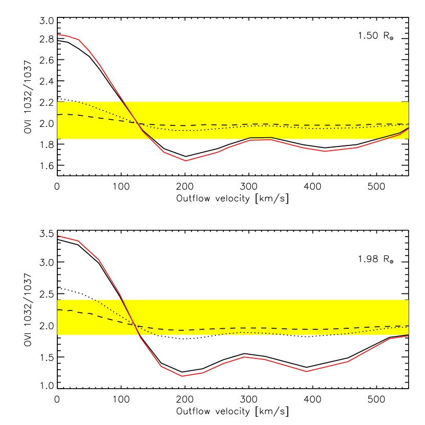
Figure 2: Model O VI (1032,1037Å) line ratio as a function of outflow velocity (in km s^-1) for the 1999 April 15 event. The dependence is shown at two heights: $1.50~{}R_{\odot}~{}(top~{}panel)$ and $1.98~{}R_{\odot}~{}(bottom~{}panel)$. The different black lines correspond to different electron densities ($n_{e}$): solid – $3.1\times 10^{6}$ and $4.6\times 10^{5}$ cm^-3, dotted – $1.6\times 10^{7}$ and $2.3\times 10^{6}$ cm^-3, dashed – $5.1\times 10^{7}$ and $7.0\times 10^{6}$ cm^-3, for two heights respectively. We chose the $n_{e}$ values so they correspond to the background coronal hole (Guhathakurta & Holzer 1994), background streamer (Guhathakurta & Fisher 1995) and several times that of the background streamer. The O VI line ratios were computed using an electron temperature, $T_{e}=5\times 10^{5}$ K. The red lines correspond to the same $n_{e}$ as the black lines but with $T_{e}=1.2\times 10^{6}$ K. It shows that the ratios do not depend significantly on the choice of $T_{e}$. The yellow block corresponds to values allowed by observations.

At $1.50~{}R_{\odot}$ UVCS recorded strong relative brightening of the O VI emission lines and only weak brightening of the H I Ly$\alpha$ (Table 2). It suggests that the H I Ly$\alpha$ enhancement was most likely reduced due to Doppler dimming. Doppler dimming arises from a Doppler shift between the incident chromospheric radiation and the moving coronal gas. The faster the gas moves, the larger the Doppler shift of its absorption profile, and thus fewer photons are scattered to form the emission line. Doppler dimming affects only the resonantly scattered part of the line. The coronal H I Ly$\alpha$ emission is strongly affected because it is mostly resonantly scattered, while the O VI lines have substantial collisional components. The model was able to reproduce all the observational parameters: the H I Ly$\alpha$ and O VI intensities as well as the $1/e$ widths of the H I Ly$\alpha$ and O VI profiles. The required electron density in the CME at $1.50~{}R_{\odot}$ was $n_{e}\approx 1.6\times 10^{7}$  cm^-3 and the required outflow velocity was $\approx 230$ km s^-1, which agrees well with with the acceleration scenario. The best fit to the electron temperature was $T_{e}=9\times 10^{5}$ K, where we assumed oxygen and hydrogen ionization equilibrium. Figure 3 shows the model prediction for the H I Ly$\alpha$ and O VI $\lambda\lambda 1032,1037$ line intensities for different $n_{e}$ and $T_{e}$ ranging from $0.5\times 10^{6}$ K and $1.5\times 10^{6}$ K at $1.98~{}R_{\odot}$. The best fit to the observed values required $n_{e}\approx 6.1\times 10^{6}$, $T_{e}=0.5-1\times 10^{6}$ K, and the CME outflow velocity ranging from 240 to 140 km s^-1 where the higher velocities correspond to lower electron temperature. Higher electron temperatures (see solution for $1.5\times 10^{6}$ K) are still marginally within the range allowed by observations but they yield low outflow velocities ($\sim 85$ km s^-1). To reproduce the observed line widths at both heights we assumed $T_{\perp}$ to be equal to the kinetic temperature derived from the H I Ly$\alpha$ and O VI $1/e$ line widths and we set $T_{\perp}=T_{\parallel}$. Coulomb collisions are expected to be strong enough to maintain isotropic velocity distribution in these dense enhancements.

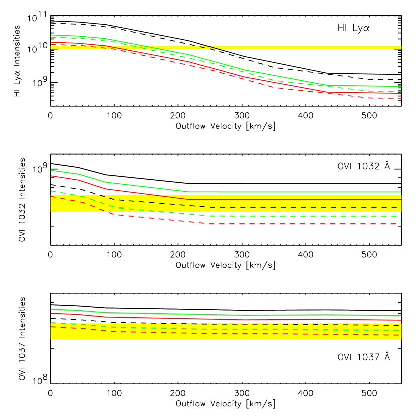
Figure 3: Model H I Ly$\alpha$ and O VI ($\lambda\lambda 1032,1037$) intensities as a function of outflow velocity for the 1999 April 15 event at $1.98~{}R_{\odot}$. The line intensities are in photons s^-1 cm^-2 sr^-1 and velocities in km s^-1. As in Figure 2, the different line styles correspond to different electron densities: $7.0\times 10^{6}$, solid, and $5.9\times 10^{6}$ cm^-3, dashed. Predictions for different electron temperatures are marked with different colors: $T_{e}=0.5\times 10^{6}$ K - black, $T_{e}=1\times 10^{6}$ K - green, and $T_{e}=1.5\times 10^{5}$ K - red. The yellow block corresponds to observationally allowed values.

3.2 1999 May 09 – unstructured CME

On 1999 May 09 UVCS recorded brightening of the emission lines at $1.38,1.58$ and $1.86~{}R_{\odot}$ by $15-28$% for the H I Ly$\alpha$ and $25-50$% for the O VI respectively (Table 2). The $1/e$ widths of the H I Ly$\alpha$ remained unchanged while the O VI profiles appeared only slightly narrower (by $5-10$ km s^-1) than the pre–CME corona. At $1.58~{}R_{\odot}$, within the uncertainties of the observed values, we obtained the best fit for $n_{e}=1.2\times 10^{7}$ cm^-3, $T_{e}\approx 1-1.2\times 10^{6}$ K and speeds of $\approx 150-115$ km s^-1, where the higher speeds correspond to lower electron temperatures. The model was able to reproduce the observed values at $1.86~{}R_{\odot}$ with $n_{e}=4.1\times 10^{6}$ cm^-3, electron temperature in a range of $T_{e}\approx 0.5-1\times 10^{6}$ K and corresponding outflow speeds of $\approx 250-150$ km s^-1. The ion temperature was set to $T_{\perp}=T_{\parallel}$

3.3 Jets or Flux Ropes

The prevalent physical models for CMEs and jets are quite different. MHD models of CMEs show plasma lifted by the upward motion of transverse magnetic field lines, (e.g. Antiochos et al. 1999), with the field lines in the form of a flux rope in many models (e.g. Gibson & Low 1998; Amari et al. 2000; Lin & Forbes 2000; Manchester et al. 2002). Jets, on the other hand, are imagined to involve strong heating at the injection site (e.g. Shimojo et al. 1996), but relatively cool material may be ejected. Kahler, Reames & Sheeley (2001) have suggested that flare-generated energetic particles observed at 1 AU are associated with narrow CMEs because these involve reconnection onto open field lines. This would suggest that narrow CMEs are more powerful versions of jets.

In the standard CME picture, reconnection will produce some local heating, but the models do not require heating for the bulk of the ejected gas. On the other hand, strong heating is observed at the ejection site (e.g. Filippov & Koutchmy 2002) and continued heating is inferred from the temperatures and ionization states observed at several solar radii (Akmal et al. 2001; Ciaravella et al. 2001). Observations of polar coronal jets also indicate continued heating as the plasma moves upward through the corona (Dobrzycka et al. 2000).

We have good diagnostic information for 2 CMEs, one structured and one unstructured. They have very similar densities and temperatures. The densities and temperatures are somewhat higher than those obtained by Dobrzycka et al. (2002) for polar coronal jets, but only by a factor of 2 or less. CMEs show a large range of temperatures as indicated by ions ranging from C III to Fe XXI (Raymond 2002), and densities are comparable to those inferred for the 1999 April 15 and 1999 June 3 events (e.g. Ciaravella et al. 2001) or higher. The speeds derived for the narrow ejections observed here are comparable to those of polar hole jets (Dobrzycka et al. 2000, 2002), and in the low to moderate speed range of CMEs. There is no obvious line width or velocity signature, such as the rotation observed in some CMEs (Ciaravella et al. 2000; Pike & Mason 2002). However, the acceleration of the 1999 April 15 event is similar to that observed in slow CMEs, but not typical of jets (Wang et al. 1998, Wood et al. 1999). This strongly indicates that the structured event is similar to larger CMEs rather than jets.

Overall, we conclude that the UVCS observations do not definitively place the narrow CMEs into the jet picture of reconnection onto open field lines or the CME picture of expanding closed field structures. If anything, their parameters are intermediate between those of jets and of CMEs. The higher sensitivity, spatial and temporal resolution of the proposed Advanced Spectroscopic and Coronagraphic Explorer (ASCE) mission should either break the structured narrow CMEs down into sinuous filaments like those observed in larger CMEs or else reveal line intensity diagnostics indicating impulsive heating at the injection site. In the mean time, a brighter event observed with a fortunate choice of observing parameters might allow the SOHO instruments to differentiate between the jet and CME pictures.

4 Summary

We presented UVCS observations of five narrow CMEs. They were among 15 narrow CMEs originally selected by Gilbert et al. (2001) based on their white light morphology and disk association. Two events (1999 March 27, April 15) were structured, i.e. in white light data they exhibited well defined interior features, and three (1999 May 9, May 21, June 3) were unstructured, i.e. appeared featureless. In UVCS data the events appeared as enhancements of the strongest coronal lines H I Ly$\alpha$ and O VI $\lambda\lambda 1032,1037$. They were $4^{\circ}-13^{\circ}$ wide and their signature was recorded at several heights. Observations by the EIT and SXT instruments suggest that the narrow CMEs are associated with disk activity that lasted up to several hours. In the LASCO C2 field of view each CME structure was visible for an extended period of time of about $1-1.5$ hour.

We derived the electron densities for several of the events from the LASCO C2 white light observations (Table 3). They are $1.5-3\times 10^{6}$ cm^-3 for the 1999 April 15 and 1999 June 3 events, which is comparable to densities inferred for regular CMEs (e.g. Ciaravella 2001). The narrow ejection on 1999 May 9 appeared to be less dense, $4.5\times 10^{5}$ cm^-3.

We used a spectral line synthesis code based on the code developed by Cranmer et al. (1999) to model plasma properties of the best observed examples of the structured and unstructured narrow CMEs. The CMEs were described as flux tubes located in the plane of the sky with no contribution from the ambient corona. We modeled the best observed examples of structured (1999 April 15) and unstructured (1999 May 9) narrow CMEs. We fit the H I Ly$\alpha$ and O VI $\lambda\lambda 1032,1037$ intensities, the $1/e$ widths as well as the O VI line ratios at each selected height.

For the April 15 event we obtained the best fit for $n_{e}\approx 1.6\times 10^{7}$ cm^-3, $T_{e}\approx 9\times 10^{5}$ K and outflow velocity of $\approx 230$ km s^-1 at $1.50~{}R_{\odot}$, which agrees with the acceleration scenario, and $n_{e}\approx 6.1\times 10^{6}$ cm^-3, $T_{e}\approx 0.5-1\times 10^{6}$ K with the CME speed from 240 to 140 km s^-1 (where the higher speed corresponding to lower $T_{e}$) at $1.98~{}R_{\odot}$.

The best fit to the May 9 observations at $1.58~{}R_{\odot}$ required $n_{e}=1.2\times 10^{7}$ cm^-3, $T_{e}\approx 1-1.2\times 10^{6}$ K and speeds of $\approx 150-115$ km s^-1, where the higher speeds correspond to lower electron temperatures. At $1.86~{}R_{\odot}$ the model was able to reproduce the observed values with $n_{e}=4.1\times 10^{6}$ cm^-3, electron temperature in the range of $T_{e}\approx 0.5-1\times 10^{6}$ K and corresponding outflow speeds of $\approx 250-150$ km s^-1, assuming an ion temperature equal to $T_{\perp}=T_{\parallel}$. Gilbert et al. (2001) found the speed of the CME to be 318 km s^-1 within the C2 field of view.

The derived plasma parameters for the structured and unstructured narrow CMEs look very similar. Compared to the polar coronal jets they have comparable speeds, higher densities and temperatures but only by a factor of 2 or less. With respect to the CMEs showing a large range of densities, temperatures and outflow speeds the narrow ejections’ plasma parameters look comparable. We did not see any obvious line width and velocity signature, such as rotation characteristic for some CMEs. However, the acceleration of the 1999 April 15 event is similar to that observed in slow CMEs, but not typical of jets (Wang et al. 1998, Wood et al. 1999).

Overall, we found that the UVCS observations do not definitively place the narrow CMEs into the jet picture of reconnection onto open field lines or the CME picture of expanding closed field structures. Additional observations of brighter events with more suitable observing parameters or with more sensitive instruments might allow us to differentiate between the jet and CME scenarios.

Table 1: UVCS/SOHO Observations of Narrow CMEs

	UVCS				LASCO C2
Date	$\rho$	P.A.	$\Delta\phi$	$t_{app}\tablenotemark{c}$	P.A.	$\Delta\phi$	$t_{app}$	Speed
	$R_{\odot}$	deg	deg	UT	deg	deg	UT	km s-1
03/27/99	1.49	314	13	16:02	310	12	16:54	475
	1.85	312	10	16:29
04/15/99	1.38	109	7	07:33	102	10	07:54	523
	1.50	108	7	07:40
	1.62	107	7	07:47
	1.74	107	7	07:59
	1.98	106	6	08:10
	2.33	105	6	08:24
	2.88	104	6	08:42
	3.62	102	5	09:27
05/09/99	1.38	100	4	19:17	100	4	19:30	318
	1.58	100	4	19:24
	1.86	100	4	19:32
	2.15	100	4	19:43
05/21/99	3.62	289		02:08	290	8	02:06	241
06/03/99	2.88	86	4	10:15	90	4	07:26	308

Table 2: Emission Line Properties

		H I Ly$\alpha$				O VI $\lambda 1032$				O VI $\lambda 1037$
Date	$\rho$	$I$	$I/I_{b}$	$V_{1/e}$	$V_{1/e}/V_{1/e,b}$	$I$	$I/I_{b}$	$V_{1/e}$	$V_{1/e}/V_{1/e,b}$	$I$	$I/I_{b}$	$V_{1/e}$	$V_{1/e}/V_{1/e,b}$
03/27/99	1.49	1.0e11	0.32	145	1	3.0e9	0.16	65	1	1.3e9	0.2	70	0.93
	1.85	2.7e10	0.38	150	1	1.3e9	0.60	60	1.1	7.1e8	1.0
04/15/99	1.38	4.5e10	0.25	101	0.65	7.8e9	1.15	74	1.06	3.4e9	1.4	74	1.05
	1.50	3.6e10	0.35	149	0.96	4.0e9	1.02	69	0.98	2.1e9	1.5	70	0.97
	1.62	2.2e10	0.37	138	0.92	2.8e9	1.75	72	0.90	1.1e9	1.92	73	0.85
	1.74	1.7e10	0.41	160	1.02	1.5e9	2.29	77	0.97	7.0e8	$\sim 3$	72	1.0
	1.98	1.1e10	0.50	135	0.87	7.0e8	3.5	82	1.00	3.1e8		82	1.0
	2.33	4.1e9	0.41	134	0.81	2.2e8	$\sim 4$			$\sim 1e8$
	2.88	8.7e8	0.27	165	1.0	3.3e7	2.4			1.6e7
	3.62	3.9e8	0.35			1.3e7
05/09/99	1.38	1.1e11	0.26	142	1.0	9.2e9	0.35	62	0.87	4.5e9	0.5	70	1.0
	1.58	4.8e10	0.28	145	1.0	2.5e9	0.30	67	0.84	1.2e9	0.4	75	1.0
	1.86	1.0e10	0.17	145	$\sim 1$	3.1e8	0.20	70	0.80	1.5e8	0.25
	2.15					$\sim 3$e8	0.6			$\sim 1$e8	0.6
05/21/99	3.62						0.5
06/03/99	2.88	8.6e8	0.12			6.9e7	0.75			2.7e7	0.96

Table 3: Electron Densities of Narrow CMEs

Date	Time	Aver. height	$\Delta\phi$	$N_{e}$
	UT	$R_{\odot}$	deg	$cm^{-3}$
04/15/99	07:54	2.77	1.9	3.0e6
	08:06	2.88	2.2	3.0e6
	08:30	3.30	2.2	2.7e6
	08:54	3.53	4.0	1.3e6
	09:06	3.65	5.0	1.1e6
	09:30	3.92	5.5	1.1e6
05/09/99	19:28	2.91	5.2	4.4e5
	19:51	3.37	4.5	4.5e5
	20:27	3.87	4.4	4.3e5
06/03/99	07:26	2.45	2.8	1.4e6
	07:50	2.85	4.7	1.3e6
	08:06	3.14	5.3	8.8e5
	08:26	3.42	4.8	8.0e5