Simulations of early structure formation: primordial gas clouds

Abstract

We use cosmological simulations to study the origin of primordial star-forming clouds in a $\Lambda$CDM universe, by following the formation of dark matter halos and the cooling of gas within them. To model the physics of chemically pristine gas, we employ a non-equilibrium treatment of the chemistry of 9 species (e^-, H, H⁺, He, He⁺, He⁺⁺, H₂, H${}_{2}^{+}$, H^-) and include cooling by molecular hydrogen. By considering cosmological volumes, we are able to study the statistical properties of primordial halos and the high resolution of our simulations enables us to examine these objects in detail.

In particular, we explore the hierarchical growth of bound structures forming at redshifts $z\approx 25-30$ with total masses in the range $\approx 10^{5}-10^{6}M_{\odot}$. We find that when the amount of molecular hydrogen in these objects reaches a critical level, cooling by rotational line emission is efficient, and dense clumps of cold gas form. We identify these “gas clouds” as sites for primordial star formation. In our simulations, the threshold for gas cloud formation by molecular cooling corresponds to a critical halo mass of $\approx 5\times 10^{5}h^{-1}M_{\odot}$, in agreement with earlier estimates, but with a weak dependence on redshift in the range $z>16$. The complex interplay between the gravitational formation of dark halos and the thermodynamic and chemical evolution of the gas clouds compromises analytic estimates of the critical H₂ fraction. Dynamical heating from mass accretion and mergers opposes relatively inefficient cooling by molecular hydrogen, delaying the production of star-forming clouds in rapidly growing halos.

We also investigate the impact of photo-dissociating ultra-violet (UV) radiation on the formation of primordial gas clouds. We consider two extreme cases by first including a uniform radiation field in the optically thin limit and secondly by accounting for the maximum effect of gas self-shielding in virialized regions. For radiation with Lyman-Werner band flux $J>10^{-23}$ erg s^-1 cm^-2 Hz^-1 str^-1, hydrogen molecules are rapidly dissociated, rendering gas cooling inefficient. In both the cases we consider, the overall impact can be described by computing an equilibrium H₂ abundance for the radiation flux and defining an effective shielding factor.

Based on our numerical results, we develop a semi-analytic model of the formation of the first stars, and demonstrate how it can be coupled with large $N$-body simulations to predict the star formation rate in the early universe.

1. Introduction

The first stars in the Universe almost certainly originated under conditions rather different from those characterizing present-day star formation. Because elements heavier than lithium are thought to be produced exclusively through stellar nucleosynthesis, the primordial gas must have been chemically pristine, presumably resulting in stars of unusually low metallicity. The recent discovery of an ultra metal-poor star by Christlieb et al. (2002) suggests that stellar relics from this era exist even today in our own Galaxy. Such old stars offer invaluable information about the history of structure formation and the chemical composition of the gas in the very early Universe.

The study of the cooling of primordial gas and the origin of the first baryonic objects has a long history (e.g., Matsuda, Sato & Takeda 1969; Kashlinsky & Rees 1983; Couchman & Rees 1986; Fukugita & Kawasaki 1991; Tegmark et al. 1997). Within the framework of the currently favored paradigm for the evolution of structure, i.e. hierarchical growth by gravitational instability, low mass halos ($\sim 10^{6}M_{\odot}$) dominated by Cold Dark Matter (CDM) seed the collapse of primordial gas within them by molecular hydrogen cooling. Numerical studies of the formation of primordial gas clouds and the first stars indicate that this process likely began as early as $z\approx 30$ (Abel, Bryan & Norman 2002; Bromm, Coppi & Larson 2002). In these simulations, dense, cold clouds of self-gravitating molecular gas develop in the inner regions of small halos and contract into proto-stellar objects with masses in the range $\approx 100-1000M_{\odot}$.

While these investigations support the notion that the first stars were unusually massive, the simulations to date have either mostly been limited to special cases or ignored the cosmological context of halo formation and collapse. In particular, the question of how the population of the first luminous objects emerged within a large cosmological volume has not been explored.

Planned observational programs will exploit future instruments such as JWST and ALMA to probe the physical processes which shaped the high-redshift Universe. Among the relevant scientific issues are the star formation rate at high redshift (e.g., Barkana & Loeb 2001; Springel & Hernquist 2003a), the epoch of reionization (e.g., Gnedin 2000; Fan et al. 2001; Cen 2002; Venkatesan et al. 2003; Sokasian et al. 2003; Wyithe & Loeb 2003a), and the fate of high-redshift systems (White & Springel 1999). The statistical properties of early baryonic objects are of direct relevance to understanding the significance of the first stars to these phenomena. In this context, the key theoretical questions can be summarized as when and where did a large population of the first stars form? and how and when did the Universe make the transition from primordial to “ordinary” star formation?

Semi-analytic modeling has often been used to address these questions qualitatively (see, e.g., Loeb & Barkana 2001). Using a spherical collapse model, Tegmark et al. (1997) estimated the critical H₂ mass fraction needed for cooling of primordial gas and a corresponding halo mass scale within which this gas can collapse. Abel et al. (1998) and Fuller & Couchman (2000) later used three-dimensional simulations to give refined estimates for the minimum collapse mass (but only for a single or a few density peaks). These results form the basis for “minimum collapse mass” models in which it is assumed that stars are formed only in halos with mass above a certain threshold. Using such a treatment, Barkana & Loeb (2000) and Mackey et al. (2003) estimated the star formation rate and supernova rate at high redshift, and Santos, Bromm & Kamionkowski (2002) computed the contribution to the cosmic infrared background from massive stars in the early Universe. Predictions from these theoretical models are, however, quite uncertain, because of the relatively crude assumptions that are used to relate the attributes of luminous objects to those of dark matter halos.

A few attempts have been made to numerically model early structure formation in cosmological volumes. Jang-Condell & Hernquist (2001) simulated a cosmological box $1$ Mpc across and found that low mass ($M\sim 10^{6}M_{\odot}$) dark matter halos at $z\sim 10$ are quite similar in their properties to larger ones at lower redshifts. However, they did not include the gas component and hence could not directly address the nature of the first baryonic objects. Ciardi et al. (2000) used outputs from $N$-body simulations to locate star-forming systems in a cosmological volume. More recently, Ricotti et al. (2002a,b) performed cosmological simulations including radiative transfer to compute the star formation history at high redshift.

Feedback processes from the first stars likely played a crucial role in the evolution of the intergalactic medium and (proto-)galaxy formation, but the detailed consequences of these effects remain somewhat uncertain. Radiation can produce either negative feedback, by dissociating molecular hydrogen via Lyman-Werner resonances (Dekel & Rees 1987; Haiman, Abel & Rees 2000; Omukai & Nishi 1998, 1999), or positive feedback from X-rays which can promote H₂ production by boosting the free electron fraction in distant regions (Haiman, Rees & Loeb 1996; Oh 2001). It is not clear whether negative or positive feedback dominates. Machacek, Bryan & Abel (2001) examined the the former using numerical simulations which included an H₂ photo-dissociating radiation field of constant flux in the optically thin limit. Cen (2002) emphasized the positive impact of an early X-ray background on the formation of the first stars and discussed the possibility that the Universe could have been re-ionized at an early epoch by Population III objects alone (see also Wyithe & Loeb 2003a, 2003b). Using three-dimensional adaptive mesh refinement (AMR) simulations, Machacek et al. (2003) further argued that the net effect of an X-ray background on gas cooling is milder than one naively expects from simple analytic estimates.

The formation of the first stars, the evolution of early cosmic radiation fields, and the thermal properties of the high-redshift intergalactic medium (IGM) are closely linked, and it is likely that semi-analytical studies of the formation of pre-galactic objects are limited by the complex cross-talk between them. Clearly, high-resolution simulations in a proper cosmological context are needed to advance our understanding of the details of first structure formation in the early Universe.

In the present paper, the first in a series on early structure formation, we study the cooling and collapse of primordial gas in dark halos using high resolution cosmological simulations. We evolve the nonequilibrium rate equations for 9 species and include the relevant gas heating and cooling in a self-consistent manner. From a large sample of dark halos, we determine conditions under which the first baryonic objects form. We show that “minimum collapse mass” models are a poor characterization of primordial gas cooling and gas cloud formation, because these processes are significantly affected by the dynamics of gravitational collapse. We also examine the influence of H₂ dissociating radiation in the form of a uniform background field in the optically thin limit as well as by approximately accounting for gas self-shielding. We quantify the overall negative effect of photo-dissociating radiation using both the numerical results and analytic estimates for the efficiency of gas cooling. Based on the simulation results, we develop a semi-analytic model to describe the formation of star-forming gas clouds in dark matter halos. To this end we adopt a simple star-formation law and compute the global star-formation rate using a large $N$-body simulation.

The paper is organized as follows. In section 2 we describe our numerical simulations. Section 3 presents general results of the simulations, ignoring radiation. Sections 4, 5 and 6 give basic properties of the dark matter halos found in our simulations. We discuss the impact of far UV radiation on primordial gas cooling in section 7. We describe a semi-analytic model for early star formation and its applications in section 8. Concluding remarks are given in section 9.

Table 1Simulation parameters

Run	$N_{\rm tot}$	L ($h^{-1}$kpc)	$m_{\rm gas}$ ($h^{-1}M_{\odot}$)	$l_{\rm s}$ ($h^{-1}$pc)
A	2$\times 288^{3}$	600	100.0	54
B	2$\times 216^{3}$	300	29.6	36
C1	2$\times 144^{3}$	300	100.0	54
C2	2$\times 144^{3}$	300	100.0	54
DM	$324^{3}$	1600	($m_{\rm DM}$) 10000.0	200

2. The $N$-body/SPH simulations

We use the parallel $N$-body/SPH solver GADGET (Springel, Yoshida & White 2001), in its “conservative entropy” formulation (Springel & Hernquist 2002). We follow the non-equilibrium evolution of nine chemical species (e^-, H, H⁺, He, He⁺, He⁺⁺, H₂, H${}_{2}^{+}$, H^-) using the method of Abel et al. (1997) and we employ the cooling rate of Galli & Palla (1998) for molecular hydrogen cooling. The time stepping method employed in the SPH simulations is described in the Appendix.

The largest of our chemo-hydrodynamic simulations (Run A) employs 48 million particles in a periodic cosmological box of $600h^{-1}$kpc on a side. We consider a conventional $\Lambda$CDM cosmological model with matter density $\Omega_{0}=0.3$, cosmological constant $\Omega_{\Lambda}=0.7$ and present expansion rate $H_{0}=70$km s^-1Mpc^-1. The baryon density is $\Omega_{\rm b}=0.04$. The initial power spectra for the baryonic and dark matter components are accurately computed from the Boltzmann code of Sugiyama (1995), in which the pressure term of baryon perturbations is taken into account. The initial power spectrum is normalized by setting $\sigma_{8}=0.9$, and all of our simulations are started at $z=100$. The initial ionization fraction was computed using RECFAST (Seager, Sasselov & Scott 2000) and was set to be $x_{e}=2.984\times 10^{-4}$ for the $\Lambda$CDM universe we adopt. Details of the set-up of the initial conditions will be presented elsewhere (Yoshida, Sugiyama & Hernquist 2003).

The basic simulation parameters are listed in Table 1. There, $L$ is the simulation box side length, $m_{\rm gas}$ is the mass per gas particle, and $l_{\rm s}$ is the gravitational softening length. Run B was carried out with a higher mass and spatial resolution to check the convergence of our numerical results. It started from the same initial matter distribution as that of C1 on large scales. Runs C1 and C2 differ only in the assigned phase information and fluctuation amplitudes in the initial random Gaussian fields. They are used to test how sample variance of the initial density field affects the final results. We carried out a simulation with dark matter only, denoted “Run DM”, to construct halo merger histories to construct the semi-analytic model described in section 8. We continued the simulations until about 100 million years after the first bound object formed. Radiation from the first object(s) should, in principle, be included because it affects the chemical and thermodynamic evolution of the surrounding IGM in a large fraction of our simulated regions. Nevertheless, we do not take such radiative effects into account in the first series of our simulations, in order to isolate other dynamical effects on primordial gas cloud formation. We carry out the same set of simulations with UV radiation in the Lyman-Werner bands and examine the global effect of photo-dissociation in section 7.

During the simulations, we save 64 snapshots of the particle data spaced logarithmically in cosmic expansion parameter from redshift $z=100$ to $z=14$. We use these outputs to identify cold, dense gas clouds, and to construct dark matter halo merger trees. We locate dark matter halos by running a friends-of-friends (FOF) groupfinder with linking parameter $b=0.164$ (Jenkins et al. 2001) in units of mean particle separation, and discard the groups which have less than 100 dark matter particles. We define the virial radius $R_{\rm vir}$ of a halo as the radius of the sphere centered on the most bound particle of the FOF group having overdensity 180 with respect to the critical density. The virial mass $M_{\rm vir}$ is then the enclosed mass (gas + dark matter) within $R_{\rm vir}$.

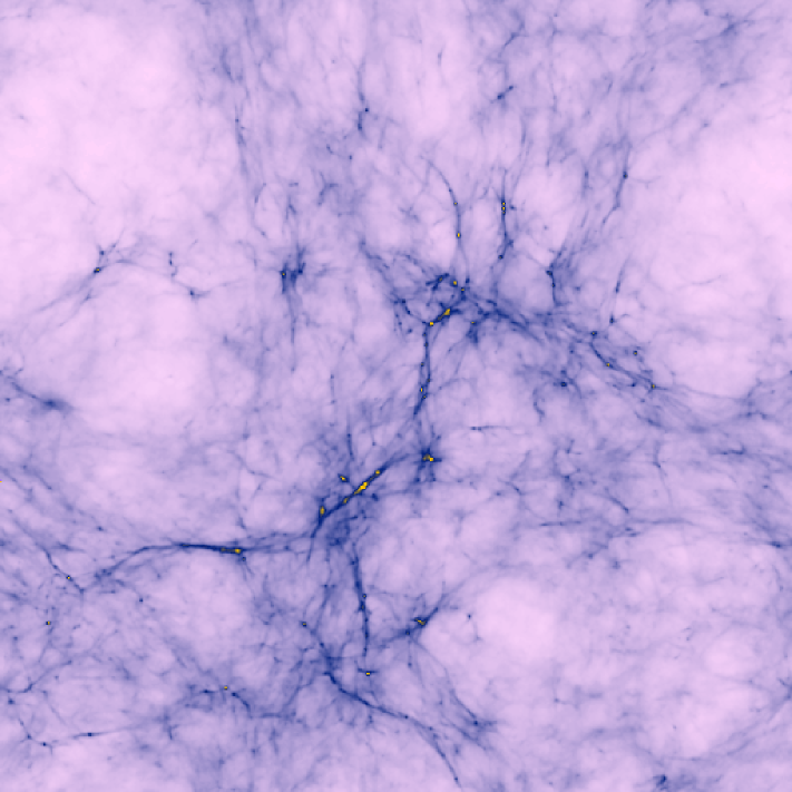
Figure 1.— The projected gas distribution in the simulation box for Run A at $z=17$. The cooled dense gas clouds appear as bright spots at the intersections of the filamentary structures.

3. The minimum collapse mass

For the halos identified in the simulations, we measure the mass of gas which is cold ($T<0.5T_{\rm vir}$) and dense ($n_{\rm H}>5\times 10^{2}$cm^-3). Once the gas starts to cool, clouds of molecular gas grow rapidly at the centers of halos and their masses exceed the characteristic Jeans mass $M_{\rm J}\sim 3000M_{\odot}$ for the typical temperature $T\sim 200$ K and density $n_{\rm H}\sim 10^{3}$cm^-3 of the condensed primordial gas. Hence, they are expected to be sites for active star formation. Hereafter, we refer to such cold, dense gas clumps as “gas clouds.” Since a halo can host more than one gas clouds, we run a FOF groufinder independently to the gas particles with a very small linking parameter $b=0.05$. In this manner we can separate groups of dense gas particles. We then discard groups of gas particles that do not satisfy the above criteria of cold, dense gas. By checking the locations of the selected groups in all the outputs, however, we found no halos which host more than one gas clouds in this particular simulation. Figure 2 shows the projected gas distribution in the simulation box of Run A at $z=17$. The bright spots are the primordial gas clouds. There are 31 gas clouds in the simulated volume. It is important to note that, whereas most of them are strongly clustered in Figure 2.— The minimum mass of the halos that host cold gas clumps. The solid lines with symbols indicate the minimum mass at the output redshifts, and the dashed lines show the mass evolution of the most massive halo in each run.
high density regions, reflecting the clustering of the underlying dark matter, some gas clouds are found in less dense, isolated regions.

In Figure 3 we plot the minimum mass of the halos that host gas clouds at each output redshift. It approximates the evolution of the minimum mass of the star-forming systems. In the figure, we also show the evolution of the most massive halo in each run. The apparent earlier formation epoch of the first bound object in Run A is simply due to finite volume effects. Run A simulated a volume 8 times larger than the others, and thus it contained a higher-$\sigma$ density fluctuation than Runs C1 or C2. Cosmic variance also explains the difference in the minimum mass between Runs C1 and C2. The assigned initial power spectrum for Run C1 had, by chance, somewhat larger amplitudes than for Run C2 on the largest scales. We checked that the dark halo mass functions are noticeably different at large mass scales between the two runs. On the other hand, excellent agreement is found in the minimum mass scale between the high resolution Run B (dot-dashed line) and low resolution Run C1 (filled circles). Our result appears to be converged on mass scales which our simulations probe.

Figure 3 clearly shows that the minimum collapse mass scale lies at $M_{\rm cr}=5\times 10^{5}h^{-1}M_{\odot}$, with only a weak dependence on redshift in the range plotted. Our result agrees reasonably well with that of Fuller & Couchman (2000), who carried out three-dimensional simulations for single high-$\sigma$ density peaks. The weaker redshift dependence found by us reflects the fact that we define the minimum collapse mass using a large sample of halos formed in various places in the simulation volume, rather than for a single or a few objects in high density regions. Our result is also roughly consistent with that of Machacek et al. (2001; 2003), who obtain a smaller value for the minimum mass, $\sim 2-3\times 10^{5}h^{-1}M_{\odot}$.

An important quantity that determines the onset of gas cooling is the fraction of hydrogen molecules, $f_{\rm H_{2}}$. In Figure 3 we plot $f_{\rm H_{2}}$ against the virial temperature for halos

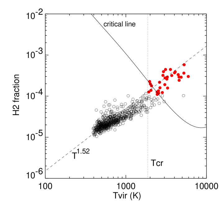
Figure 3.— The mass weighted H₂ fraction versus virial temperature for the halos that host gas clouds (filled circles) and for those that do not (open circles) in Run A at $z=17$. The virial temperature is related to the halo mass by equation (1). The solid curve is the H₂ fraction needed to cool the gas at a given temperature and the dashed line is the asymptotic H₂ fraction.

in Run A at $z=17$. We compute the virial temperature for the halo mass using

$$T = 1.98\times 10^{4}\left(\frac{\mu}{0.6}\right)\left(\frac{M_{\rm halo}}{10^{8}h^{-1}M_{\odot}}\right)^{2/3}$$

$$\left(\frac{\Omega}{\Omega_{z}}\frac{\Delta}{18\pi^{2}}\right)^{1/3}\left(\frac{1+z}{10}\right)\mbox{K},$$

where $\mu$ is the mean molecular weight and $\Delta$ is the collapse overdensity. Filled circles represent the halos harboring a cold dense gas cloud, while open circles are for the others. The solid line is an analytical estimate of the H₂ fraction needed to cool the gas, which we compute a là Tegmark et al. (1997). Briefly, we compute the characteristic cooling time of a gas with density $\rho$ and temperature $T$ as $t_{\rm cool}=k_{\rm B}T/\rho\Lambda(\rho,T)$ where $\Lambda(\rho,T)$ is the cooling rate due to molecular hydrogen rotational line transitions, and determine the critical molecular hydrogen abundance with which the gas can cool within a Hubble time. Note that we use the cooling function of Galli & Palla (1998) for our simulations and for this estimate. The dashed line is the asymptotic molecular fraction of a gas in a transition regime when electron depletion makes the production of hydrogen molecules ineffective. Then the molecular fraction scales as $f_{\rm H_{2}}\propto T^{1.52}$ (see eq. [17] of Tegmark et al. 1997)

In Figure 3, halos appear to be clearly separated into two populations; those in which the gas has cooled (top-right), and the others (bottom-left). Our analytic estimate indeed agrees very well with the distribution of gas in the $f_{\rm H_{2}}$ - $T$ plane. We emphasize, however, that this apparent agreement should not be interpreted as the model precisely describing the gas evolution. Also, the analytic model itself is expected to be accurate only to within some numerical factor.

Although the H₂ fraction primarily determines whether the gas in halos can cool or not, there are some halos within which gas clouds have not formed despite the high gas temperatures (open circles with $T>T_{\rm cr}$). At $z=17$, about 30% of the massive halos are “deficient” in this manner. Similar features are also found in the result of the AMR simulation of Machacek et al. (2001, their Fig. 3). In the next section we further examine what prevents the gas from cooling and collapsing in these halos.

4. Halo formation history

Halos in CDM models grow hierarchically through merging and the accretion of smaller objects. The complex and violent formation processes of dark halos affect the thermal and chemical evolution of the gas within them. To addess this, we study the dynamical influence of dark matter on gas cloud evolution using halo merger histories. We identified a total of 635 dark halos in Run A at $z=17$. For all the halos, we traced their progenitors in earlier outputs to construct merger trees. In Figure 4 we plot the mass evolution of a subset of halos that host gas clouds (top-left panel) and of another subset of halos that do not host gas clouds (top-right panel). In the top-left panel, we mark trajectories by filled circles when they host gas clouds. The figures show a clear difference between the two subgroups in their mass evolution. Most of the halos in the top-left panel experience a gradual mass increase since the time their masses exceeded $M_{\rm cr}$, whereas those plotted in the top-right panel have grown rapidly after $z\sim 20$. It appears that the gas in halos that accrete mass rapidly (primarily due to mergers) is unable to cool efficiently.

Rapid mass accretion and mergers dynamically heat the gas when halos form, causing it to become hot and rarefied, rather than allowing it to radiatively cool and condense. This is the situation first considered by White & Rees (1978) in the context of hierarchical galaxy formation. The simplest model to describe the evolution of radiative gas assumes that the gas cools when the characteristic cooling time is shorter than the dynamical time. This scenario has been used to estimate the minimum mass scale for galaxies. The gas cooling rate due to atomic hydrogen and helium associated with galaxy formation has a particular behavior in it decreases sharply below $T=10^{4}$ K by many orders of magnitude, which effectively prevents the cooling of gas in systems with low virial temperatures. Hence, the cooling criterion $t_{\rm cool}<t_{\rm dyn}$ simply sets a definite minimum mass scale (at a given redshift) for galaxy formation.

The situation we consider here is clearly different, because molecular hydrogen cooling is a much less efficient process and has a weaker dependence on temperature. More important, for this mechanism to be effective, a certain number of hydrogen molecules must first be produced, because the residual H₂ abundance in the early Universe is negligible. Figure 4 illustrates these features. In the bottom panels, we plot the evolution of the molecular hydrogen fraction and the mean gas mass weighted temperature for the same halos as in the top panels. Most of the trajectories in the bottom-right panels show a common feature: the temperature rises with little increase in the molecular hydrogen fraction.

We can understand this as follows. Consider an equal-mass merger where two halos each with a mass $5\times 10^{5}h^{-1}M_{\odot}$ merge to form an object of mass $10^{6}h^{-1}M_{\odot}$ at $z=20$. The H₂ fraction of the gas in the two halos is

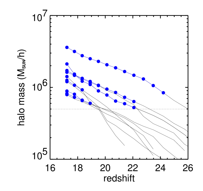
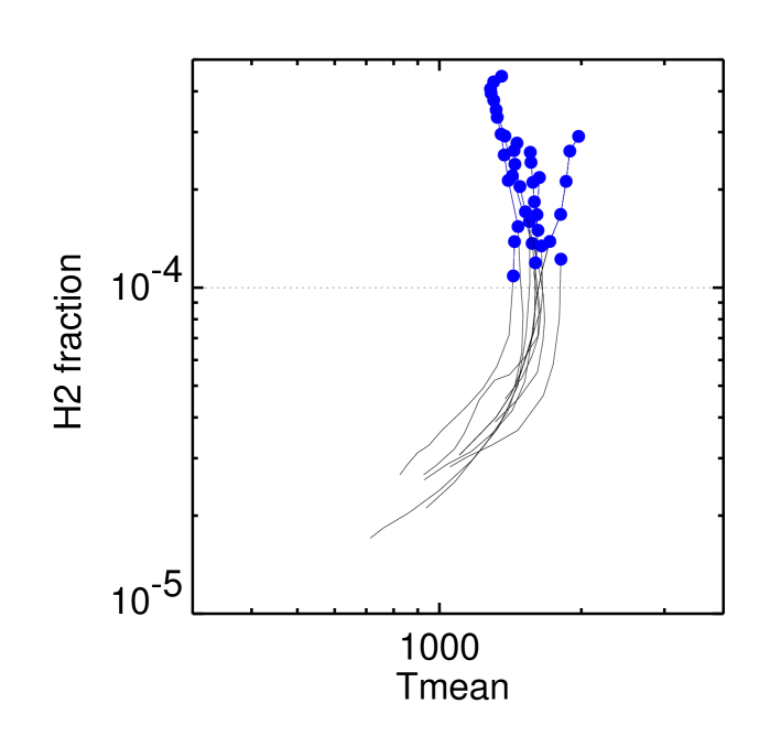
Figure 4.— Top panels: The mass evolution of the halos that host gas clouds at z=17 (left) and those that do not (right) for Run A. Bottom panels: The molecular hydrogen fraction is plotted against the mean gas-mass-weighted temperature for the same halos as in the top panels.

predicted to be about $8.0\times 10^{-5}$ (see the dashed line in Figure 3). After virialization, the gas temperature becomes $T_{\rm vir}\sim 2300$K, and our estimate for the H₂ fraction needed for the gas to cool is about $2\times 10^{-4}$, about a factor of 2.5 larger than the progenitor gas. In this case, the production of molecular hydrogen, the coolant, must precede cooling. Only when a further temperature increase or an increase in the molecular fraction brings the gas into the region above the critical line in the $f_{\rm H_{2}}-T$ plane can the gas cool efficiently, unless significant heating occurs during this cooling phase. The molecular hydrogen formation time scale for this typical halo is estimated to be

$$t_{\rm H_{2}}=\frac{n_{\rm H_{2}}}{k_{\rm H^{-}}n_{\rm H}n_{\rm e}}\approx 30{\rm Myrs},$$ (2)

where $k_{\rm H^{-}}$ is the reaction coefficient of H^- formation via H + e^- $\rightarrow$ H^- + $\gamma$. The H₂ formation timescale is comparable to the dynamical time for this halo.

It is interesting that the most massive halo plotted in the top-right panel of Figure 4 has a mass of $3.5\times 10^{6}h^{-1}M_{\odot}$ at $z=17$. The mass growth of the halo is so rapid below $z=20$, when it had a mass of $5\times 10^{5}h^{-1}M_{\odot}$, that the gas within it could not cool to form a dense gas cloud. It has been instead continuously heated dynamically. We can quantify this dynamical effect using our simulations. We trace the progenitors of the massive ($M>7\times 10^{5}h^{-1}M_{\odot}$) halos in Run A identified at $z=17$, and compute recent mass accretion rates from $\Delta M/\Delta z=(M(z_{2})-M(z_{1}))/(z_{2}-z_{1})$, where we choose $z_{1}=18.5$ and $z_{2}=17$. In Figure 4 we plot the measured mass growth rates against the halo masses. Filled circles represent the halos that host gas clouds at $z=17$, and open circles are for those that do not. We derive a critical mass growth rate by equating the heating rate to the Figure 5.— The mass growth rate versus halo mass for halos at z=18.5 in Run A. The mass growth rates are computed from $\Delta M/\Delta z=(M(z_{2})-M(z_{1}))/(z_{2}-z_{1})$, where $z_{1}=18.5$ and $z_{2}=17$. Note that, according to our definition, the mass increase per unit redshift can be larger than the halo mass itself at $z_{1}$, if the halo’s descendant is more massive (up to by a factor of two) due to successive mergers during the redshift interval considered. The solid line shows the critical instantaneous mass growth rate computed from the dynamical heating rate that balances the estimated cooling rate.
molecular hydrogen cooling rate from

$$\frac{dQ_{\rm dyn.heat}}{dt} \equiv \frac{k_{\rm B}}{\gamma-1}\frac{dT}{dt}$$

$$= \Lambda_{\rm H_{2}}(T)\times f_{\rm H_{2}}$$

$$(\mbox{cooling rate per hydrogen atom}),$$

and relate the increase in virial temperature to the mass growth rate by

$$\frac{dT}{dt}=\alpha M^{-1/3}\frac{dM}{dt},$$ (4)

where the coefficient $\alpha$ is computed from equation (1) at a given time. Strictly speaking, the temperature of the gas in a halo could be different from the halo’s virial temperature. We have carried out an additional simulation with non-radiative gas starting from the same initial conditions as Run B (the highest resolution simulation) and found that the mean gas-mass weighted temperature is indeed close to the halo’s virial temperature for almost all the halos, with deviations smaller than a factor of two (see also Figure 2 of Machacek et al. 2001). Therefore, we may safely assume that the gas temperature is close to the virial temperature before cooling occurs.

In Figure 4, the solid line is our analytic estimate for the critical mass growth rate. Above the solid line, the mass growth rate is so large that dynamical heating acts more efficiently than cooling by molecular hydrogen. Thus, in such halos, gas cloud formation is effectively delayed or prevented. Note the steepness of the critical mass growth rate, which reflects the slope of the molecular hydrogen cooling rate $\Lambda(T)\propto T^{1.5}$ in the temperature and density range of interest. For a halo with mass $5\times 10^{5}h^{-1}M_{\odot}$ at $z\sim 20$, even a 20% mass increase per unit redshift results in net heating of the gas. The critical mass growth rate

Figure 6.— Spin parameters of halos are plotted against their masses, for the dark matter component (top) and for the gas (bottom) in our largest run (Run A) at $z=17$. We plot halos with mass greater than $10^{5}h^{-1}M_{\odot}$. Filled and open circles indicate halos with and without gas clouds, respectively.

therefore sets a natural lower limit for primordial gas cloud formation at a mass scale $\sim 5\times 10^{5}h^{-1}M_{\odot}$, in good agreement with the result shown in Figure 3.

5. The angular momenta of dark matter and gas

Recent numerical studies by Bromm et al. (2002) show that the initial angular momentum of primordial gas may determine the properties of the first star-forming clouds and possibly of the stars themselves. By pre-assigning the system’s initial angular momentum and following its evolution, Bromm et al. (2002) found that a disk-like structure is formed in high spin systems and that the gas subsequently fragments. It is therefore interesting to ask whether such high spin systems are indeed produced in cosmological simulations. We measure the spin parameters of the dark matter component and of the gas within them. We follow the definition of Bullock et al. (2001):

$$\lambda=\frac{j}{\sqrt{2}R_{\rm vir}V_{\rm vir}},$$ (5)

where $j$ is the specific angular momentum of each component (dark matter or gas) and $V_{\rm vir}=\sqrt{GM_{\rm vir}/R_{\rm vir}}$ is the circular velocity at the virial radius.

In Figure 4, we plot the spin parameters of the dark matter and of the gas against the halo mass for Run A at $z=17$. For the gas component, we included all the gas (hot + cold) particles within the virial radius. The distribution of the dark matter spin parameters is quite similar to that of both high mass halos (van den Bosch et al. 2001) and small halos (Jang-Condell & Hernquist 2001). The spin parameter distribution for the dark matter is well fitted by the lognormal function

$$p(\lambda)d\lambda=\frac{1}{\sqrt{2\pi}\sigma_{\lambda}}\exp\left[-\frac{\ln^{2}(\lambda/\bar{\lambda})}{2\sigma^{2}_{\lambda}}\right]\frac{d\lambda}{\lambda},$$ (6)

with $\bar{\lambda}=0.035$ and $\sigma_{\lambda}=0.54$. We also note that the spin vectors of dark matter and the gas are not closely aligned, with a median deviation angle of $\approx 30$ degrees, in good agreement with the results of van den Bosch et al. (2001) for higher mass halos.

In Figure 4, the spin parameters appear relatively smaller for halos with gas clouds than for the entire halo population, because gas clouds form only in halos at the high-mass end. Bromm et al’s result suggests that in systems with a spin parameter as large as 0.06, gas clouds eventually flatten to form a rotationally supported disc. We find only two star-forming halos in which either the gas or dark matter spin parameters are greater than 0.06. Although rare, such objects do form in the CDM model. It is important to point out, however, that the spin vectors of the gas and dark matter are not usually aligned. This confirms the importance of setting up simulations in a proper cosmological context. Intriguingly, Vitvitska et al. (2002) argue that halos which have experienced recent major mergers tend to have high spin parameters. This may explain the overall trend in Figure 4 that gas clouds are preferentially found in low-spin halos.

It is still a difficult task to measure the spin parameters of the formed dense gas clouds accurately, because of resolution limitations. To address the question of the exact shape and the size of the final gas clump, we require a substantially higher resolution simulation.

6. Gas cloud evolution

The cooling and condensation of the gas within a dark halo can be qualitatively understood using a spherical collapse model. Following Omukai (2001), we consider a spherical gas cloud embedded in a dark halo. We assume that the dynamics of the gas sphere is described by

$$\frac{d\rho_{\rm gas}}{dt}=\frac{\rho_{\rm gas}}{t_{\rm ff}},$$ (7)

where $\rho_{\rm gas}$ is the gas density and the free fall time $t_{\rm ff}$ is given by

$$t_{\rm ff}=\sqrt{\frac{3\pi}{32G\rho}}.$$ (8)

We solve the energy equation

$$\frac{de}{dt}=-p\frac{d}{dt}\left(\frac{1}{\rho_{\rm gas}}\right)-\frac{\Lambda_{\rm cool}}{\rho_{\rm gas}},$$ (9)

together with the chemical reactions and the cooling rate computed in a consistent manner as in our simulation. Specifically, the net cooling rate $\Lambda_{\rm cool}$ includes cooling by molecular hydrogen $\Lambda_{\rm H_{2}}$, cooling by hydrogen and helium

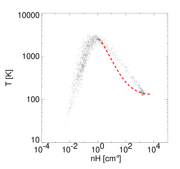
Figure 7.— The distribution of gas particles within a 200 pc (physical) radius from the center of the most massive halo in Run C1 at $z=20.7$ in the density - temperature plane. Densities are given in units of number density of hydrogen atoms per cubic centimeters. The dashed line shows the evolutionary track for spherically collapsing gas as described in section 6.

atomic transitions $\Lambda_{\rm H,He}$, and the inverse Compton cooling $\Lambda_{\rm Compton}$. Although the atomic line cooling is unimportant in the temperature range we consider, we include it for completeness.

For our purposes, we follow the evolution of the gas after it is virialized. We take the initial temperature of the collapsing gas cloud to be the virial temperature of the most massive halo in Run C1 at $z=23$, which has a mass of $6\times 10^{5}h^{-1}M_{\odot}$ and a virial temperature $T_{\rm vir}=2300$ K. We follow the thermodynamic evolution of the gas from $z=23$ to $z=20.7$. Figure 6 shows the distribution of the halo gas particles in the thermodynamic phase plane at $z=20.7$. We select the gas particles within $200$ pc (physical) of the center of the halo. The trajectory computed by solving equations (7)-(9) is shown by the dashed line. It describes the evolution of the gas from $z=23$ to $z=20.7$ reasonably well. Note that the cooling branch, appearing as dots in the right portion of the plot, does not exactly represent the evolutionary track of the gas particles. The dots show the densities and temperatures of the gas particles at the output time, $z=20.7$. The cooled primordial gas piles up near the halo center with a characteristic temperature $T\sim 100-200$K and number density $n_{\rm H}\sim 10^{3}-10^{4}$cm^-3, in good agreement with the prediction of the spherical collapse model.

7. Effect of radiative feedback

In the previous sections, we focused on the formation of the very first objects in the absence of an external radiation field. After the first stars form, they emit photons in a broad energy range. Radiation from the first stars affects not only the IGM in the vicinity of the stars, but could also build up a background radiation field in certain energy bands. Photo-dissociation of molecular hydrogen due to radiation in the Lyman-Werner (LW) bands (11.18eV - 13.6eV) is of primary importance, because the LW radiation can easily penetrate into the neutral IGM (Dekel & Rees 1987; Haiman, Abel & Rees 2000; Omukai & Nishi 1999; Glover & Brand 2001). We first model the influence of LW radiation by including a uniform radiation background in the optically thin limit, as in Machacek et al. (2001). In section 7.3, we also take into account gas self-shielding in the same set of simulations and compare the results with those for the optically thin cases.

7.1. Uniform background radiation

To begin, we adopt a constant radiation intensity in the LW band of either $10^{-23}$ or $10^{-22}$ erg s^-1 cm^-2 Hz^-1 str^-1. We use the photo-dissociation reaction coefficient given in Abel et al. (1997),

$$k_{\rm diss}=1.38\times 10^{9}J(h\nu=12.87{\rm eV}).$$ (10)

Hereafter, we describe the intensity by the conventional normalization $J_{21}$. We adopt the values $J_{21}=0.01,0.1$ by noting that the LW radiation with intensities $J_{21}\leq 0.001$ does not significantly affect the abundance of molecular hydrogen in halos, whereas radiation with $J_{21}\geq 1.0$ will quickly dissociate hydrogen molecules. This can be easily seen by computing the dissociation time scale

$$t_{\rm diss}=k^{-1}_{\rm diss}\sim\frac{10^{12}}{J_{21}}\;\;{\rm sec}.$$ (11)

During Run C1, we turned on the background radiation at $z=24$, slightly before the formation of the first gas cloud in the simulation box. Although it might seem more consistent to turn on the radiation only after the first object is formed, we start it slightly earlier, in order to study the evolution of the gas in the most massive halo as well. Figure 7.1 shows the distribution of gas particles in the thermodynamic phase plane at $z=20.7$. The dashed lines in Figure 7.1 are computed by solving equations (7)-(9) including the LW radiation with $J_{\rm 21}=0.1$ and 0.01. For these cases we computed the evolution of the abundance of molecular hydrogen $f_{\rm H_{2}}$ for $J_{\rm 21}=0.1$ and 0.01. and then evaluated the gas cooling rate $\Lambda_{\rm H_{2}}(T,f_{\rm H_{2}})$. For $J_{\rm 21}=0.01$, the cooling branch now appears to lie on a shallower line than for the case with no radiation (Figure 7). The analytic model again describes the feature reasonably well. It is interesting that under the influence of LW radiation the characteristic temperature of the gas clouds becomes higher than in the case with no radiation. Omukai (2001) argues that both the density and temperature of gas clouds in the regime before they start to undergo run-away collapse become higher for a stronger radiation field and the characteristic Jeans mass becomes smaller. Although our simulation does not probe this regime owing to lack of resolution, it is intriguing that the presence of radiation affects the final mass of the collapsing gas clouds. Note also that, in a cosmological context, even a slight delay of gas cooling can make the subsequent evolution very different because of the rapid formation of dark matter halos.

The case with $J_{21}$=0.1 is noticeably different from the other two (Figure 7, 8) models. Gas cooling and collapse are almost entirely prevented when the LW radiation dissociates molecular hydrogen. For this case, we compute the H₂ formation and dissociation timescales to be $t_{\rm H_{2}}=30$ Myrs, $t_{\rm diss}=3$ Myrs, respectively, with the latter being much smaller than the former. Thus, we expect the H₂ abundance to be close to the equilibrium value. The equilibrium H₂ abundance is then given by

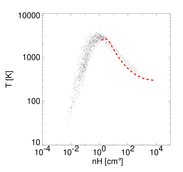
Figure 8.— The distribution of gas in the density - temperature plane for the same halo as in Figure 7, but with Lyman-Werner background radiation having flux $J_{21}=0.01$ (top) and $J_{21}=0.1$ (bottom). Evolutionary track is not shown for the latter case, because the solution does not exist for non-collapsing gas.

$$n_{\rm H_{2},eq}\approx\frac{k_{\rm H^{-}}n_{\rm H}n_{e}}{k_{\rm diss}},$$ (12)

which yields the fraction $f_{\rm H_{2}}=2\times 10^{-6}$ in the present case. It is nearly two orders of magnitude smaller than the critical fraction needed to cool the gas (see Figure 2); obviously, such gas cannot cool.

We generalize the above argument using the larger box simulation Run A. We turn on a uniform background radiation field with $J_{21}=0.01$ at $z=24$ and continue the run until $z=17$. We call this simulation “Run A-r”. Figure 7.1 shows the mean molecular hydrogen fraction against the virial temperature for the halos identified at $z=17$ in this simulation. As in Figure 3, the critical molecular hydrogen fraction to cool the gas is shown by the solid line, and the equilibrium H₂ abundance computed by equation (12) is indicated by the dashed line. For this plot, we computed the equilibrium H₂ abundance by accounting for the fact that gas densities in small halos are smaller than the universal baryon fraction times the mean matter density within halos, because of gas pressure (Loeb & Barkana 2001). The dashed line in Figure 7.1 thus appears to steepen toward the low temperature end. The agreement with the measured mean molecular fraction is quite good, although the simulated halos show a large scatter at high temperatures. Since the analytic model we adopted

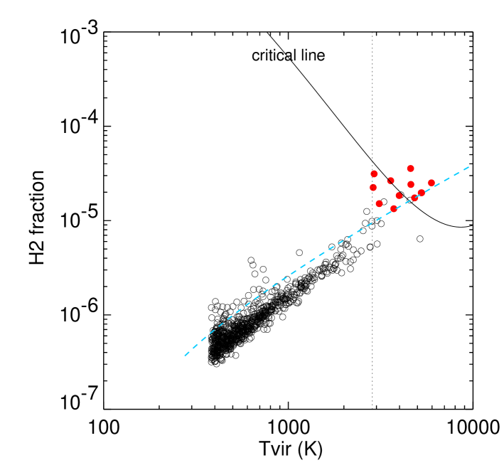
Figure 9.— As for Figure 3, but for simulation Run A-r with a background radiation in the Lyman-Werner band with $J_{21}=0.01$.

is expected to be accurate only to within some numerical factor, we plot a factor of two smaller critical H₂ abundance in Figure 7.1 (solid line) than that in Figure 3. This brings the critical curve into good agreement with the simulation results. In Figure 7.1, the critical temperature $T_{\rm cr}$ defined at the point where the critical $f_{\rm H2}$ is equal to the equilibrium H₂ abundance also agrees reasonably well with the actual minimum temperature (vertical dotted line) found in our simulation.

Overall, we find that radiative effects are quite substantial. The mean molecular hydrogen fractions drop by nearly an order of magnitude for a radiation field with $J_{21}$ = 0.01. An order of magnitude higher radiative flux will make the mean molecular fraction even smaller and make primordial gas cooling very inefficient, as we have seen in Figure 7.1.

7.2. Self-shielding

Although our simulation results in the previous section highlighted a negative aspect of radiative feedback, the true importance of this effect remains somewhat uncertain, because of our oversimplified treatment of the background field. The optically thin assumption breaks down as dense gas clouds form, requiring that self-shielding be taken into account. However, the strength of self-shielding is a difficult question to address. For a static gas it is indeed significant, giving an effective shielding factor $f_{\rm shield}\ll 1$ for molecular hydrogen column densities $N_{\rm H_{2}}\gg 10^{14}$ cm^-2 (Drain & Bertoldi 1996). For a gas with extremely large velocity gradients and disordered motion, the gas remains nearly optically thin even for column densities $N_{\rm H_{2}}\sim 10^{20-21}$cm^-2 (Glover & Brand 2001). Since the full treatment of three-dimensional radiative transfer for 76 LW lines, even when only the lowest energy level transitions are included, is practically intractable (see, however, Ricotti et al. 2001 for one-dimensional calculations for a stationary gas), we adopt the following approximate method to estimate the maximum effect of self-shielding. We consider only shielding by gas in virialized regions and do not consider absorption by the IGM in underdense

Figure 10.— Top: The gas density profile (solid line with circles) and the molecular fraction profile (dashed line) of the most massive halo in Run A at $z=25$. An isothermal density profile is also shown by the solid line. Bottom: The molecular hydrogen column density computed from the profiles in the top panel (dashed line) and the column densities evaluated at the positions of the gas particles are plotted against distance from the halo center.

regions, assuming that the amount of residual intergalactic H₂ is negligible. Although this is not true initially, the intergalactic H₂ fraction quickly decreases after the very first stars appear (Haiman, Abel & Rees 2000). On the other hand, the so-called “saw-tooth” modulation of background radiation owing to neutral hydrogen Lyman series absorption (Haiman et al. 1997) is substantial in the Lyman-Werner band because neutral hydrogen is abundant at very high redshifts. Nevertheless, we do not consider the evolution and attenuation of radiation and we fix the radiation intensity as an input, rather than computing it consistently from actual star formation. Thus the assigned intensity may be regarded as that after the radiation is attenuated by intergalactic neutral hydrogen. We consider the evolution and modulation of the radiation spectrum in section 8.

As for the simulations presented in section 7.1, we apply a background radiation field in the LW band. The radiation intensity at each position in the simulated region is computed by assuming that it is attenuated through surrounding dense gas clouds. We define a local molecular hydrogen column density $N_{\rm H_{2}}$ in a consistent manner employing the SPH formalism. We use the local molecular hydrogen abundance and Figure 11.— As for Figure 9, but for the simulation including the effect of gas self-shielding (Run A-s).
density to obtain an estimate for the column density around the $i$-th gas particle according to

$$N_{{\rm H_{2}},i}=\int_{{\bf r}_{i}}^{r_{\max}}n_{\rm H_{2}}dl$$ (13)

where ${\bf r}_{i}$ is the position of the $i$-th gas particle and $r_{\rm max}$ is the length scale we choose in evaluating the column density. In practice, we select an arbitrary line-of-sight and sum the contributions from neighboring gas particles within $r_{\rm max}$ by projecting an SPH spline kernel for all the neighboring particles whose volume intersects the sight-line. We repeat this procedure in six directions along x, y, and z axes centered at the position of the $i$-th particle and take the minimum column density as a conservative estimate. We mention that our method is similar in spirit to the local optical depth approximation of Gnedin & Ostriker (1997). We have chosen the length scale $r_{\rm max}=100$ physical parsec by noting that the virial radius of a halo with mass $10^{6}h^{-1}M_{\odot}$ is just about 100 parsec. There are not significantly larger gas clumps than this scale in the simulated region. The local column density estimates are easily computed along with other SPH variables with a small number of additional operations.

Figure 7.2 shows the gas density and molecular hydrogen fraction profiles for the most massive halo in Run A at $z=25$. The gas density profile is very close to an isothermal density profile, scaling as $\rho_{\rm gas}\propto r^{-2}$, except in the central 10 pc. In the bottom panel, we compare the estimated column densities at the position of each gas particle computed directly in the simulation (dots) with the analytic estimate (dashed line). We use the spherically averaged gas density and molecular hydrogen fraction profiles shown in the top panel and integrate from an arbitrary outer boundary as $\int_{\rm r}^{\rm r_{\rm out}}n_{\rm H}f_{\rm H_{2}}dr$, to obtain the analytic estimate $N_{\rm H_{2}}(r)$. The agreement is quite good, assuring that our technique yields accurate estimates for the column density. Following Drain & Bertoldi (1996), we parameterize the shielding factor as

$$F_{\rm shield}=\min\left[1,\left(\frac{N_{\rm H_{2}}}{10^{14}{\rm cm}^{-2}}\right)^{-3/4}\right].$$ (14)

The photo-dissociation reaction coefficient is then given by

$$k_{\rm diss}=1.38\times 10^{9}J(h\nu=12.87{\rm eV})F_{\rm shield}.$$ (15)

The bottom panel of Figure 7.2 shows that, at the halo center, the column density is close to $10^{17}$ cm^-2, and hence the radiation intensity is expected to be significantly reduced according to equation (14). It should be emphasized that the above expression for the shielding factor is derived for a stationary gas, and thus the actual effect of self-shielding could be substantially smaller because of gas velocity gradients and disordered motions, as discussed in Machacek et al. (2001). The results using the above estimate can, therefore, be regarded as describing the maximum possible effect of self-shielding.

We again use Run A. Similar to the optically thin case, we turn on a background radiation field with $J_{21}=0.01$ at $z=24$, and compute self-shielding factors for all the over-dense gas particles (hence for virtually all the gas particles in virialized regions). We call this simulation “Run A-s” (for shielding). Figure 7.2 shows the mean molecular fraction against virial temperature for halos in Run A-s at $z=17$. The mean molecular hydrogen fractions lie, with substantial scatter, on a steeper line than for the optically thin case (compare with Figure 7.1), indicating effective shielding. For large halos, indeed, the mean molecular hydrogen fractions are close to the values we found in Run A (with no radiation, see Figure 3). On the other hand, the gas in small halos is nearly optically thin, and their mean molecular fractions are close to those found in the optically thin limit (Figure 7.1). We have found that we can quantify this trend by computing an effective shielding factor

$$F_{\rm eff.shield}=F(N_{\rm H_{2}}=Cf_{\rm H2}n_{\rm H}R_{\rm vir}),$$ (16)

where the function $F$ is defined in equation (14), $f_{\rm H2}$ is computed assuming no radiation, $n_{\rm H}$ is the hydrogen number density taken to be 180 times the mean density, and $R_{\rm vir}$ is the halo’s virial radius. We have introduced a constant factor $C$. Choosing $C=0.2$ and computing the equilibrium H₂ abundance from equation (12) for the effectively attenuated radiation flux using equation (15), we have obtained molecular fractions which agree very well with the abundances found in the simulation. The dashed line in Figure 7.2 shows the equilibrium H₂ abundance calculated in this manner. A value somewhat smaller than unity was chosen for $C$ by noting that a large fraction of the gas in the outer envelope of the halos remains nearly optically thin, as can be inferred from Figure 7.2.

7.3. Minimum collapse mass under far UV radiation

The net effect of photo-dissociating radiation is to raise the minimum collapse mass scale for primordial gas cooling (Haiman et al. 2000; Machacek et al. 2001; Wyse & Abel 2003). In Figure 7.3, we plot the minimum mass of halos that host gas clouds for 3 sets of simulations. Although there are small fluctuations, the minimum mass scales remain approximately constant, at $5\times 10^{5},6.5\times 10^{5},$ and $1\times 10^{6}h^{-1}M_{\odot}$ for Run A, Run A-s, and Run A-r, respectively.

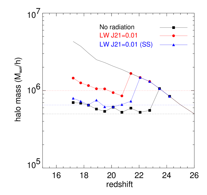
Figure 12.— Minimum mass of the halos that host gas clouds in Run A (no radiation case, squares), Run A-r (radiation flux $J_{21}=0.01$, circles), and Run A-s (radiation flux $J_{21}=0.01$ with gas self-shielding taken into account, triangles). The solid line shows the mass evolution of the most massive halo.

Figure 7.3 summarizes our findings in this section. We compute the critical H₂ fraction and the asymtotic H₂ fraction for no radiation case in the same manner as described in section 2. We also show the equilibrium H₂ abundance for two cases with the LW radiation with $J_{21}=0.01$ (thick dotted line) and with $J_{21}=0.1$ (thin dotted line) using equation (12). Finally we compute the equilibrium abundance H₂ by taking the gas self-shielding into account using equations (14)-(16). The effect of LW radiation is to reduce the fraction of molecular hydrogen, $f_{\rm H_{2}}(T_{\rm vir})$, for a given virial temperature $T_{\rm vir}$. For optically thin radiation with $J_{21}=0.01$, $f_{\rm H_{2}}(T_{\rm vir})$ is more than an order of magnitude smaller than in the case with no radiation (compare the dashed line denoted as case (a) with the thick dotted line denoted as (b)). The case with maximal gas self-shielding in our implementation lies in between these two cases and bridges the low temperature ($\sim 600$ K) end of the optically thin case and the high temperature ($\sim 4000$ K) end of the no radiation case. We expect that the true effect of gas self-shielding should lie between these two extremes. The minimum collapse mass scales for the three cases can be given, via the mass-temperature relation in equation (1), by the crossing points of these three curves with the critical molecular fraction shown by the solid line in Figure 7.3. As can be inferred from Figure 7.3, the minimum virial temperature for gas cloud formation by molecular hydrogen cooling monotonically increases for increasing radiation intensity. In the figure we also show the equilibrium molecular hydrogen abundance for optically thin radiation with $J_{21}=0.1$ by the thin dotted line. It does not cross the critical $f_{\rm H_{2}}(T)$ curve, and thus, under such high intensity radiation, molecular hydrogen cooling never becomes efficient in the entire temperature range plotted. Note, however, that in large halos with virial temperatures higher than $\simeq 7000$ K, the gas can cool by atomic hydrogen transitions. The overall cooling efficiency in large halos is then dominated by atomic cooling and will

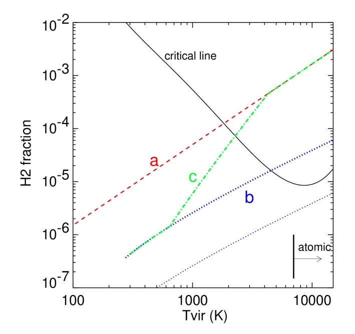
Figure 13.— The critical molecular hydrogen fraction to cool the gas (solid line), the H₂ fraction for (a) no radiation case (dashed line), (b) radiation with $J_{21}=0.01$ (thick dotted line), and (c) radiation with $J_{21}=0.01$ with an effective self-shielding factor taken into account (dot-dashed line). The thin dotted line is the equilibrium H₂ abundance for a radiation flux $J_{21}=0.1$. These are computed at $z=17$. The vertical line shows the virial temperature above which atomic hydrogen line cooling becomes efficient.

not be critically affected by the H₂ dissociating radiation regardless of its intensity.

7.4. Processes neglected

Throughout this section we have considered radiation only in the Lyman-Werner bands. While photons with energy above 13.6eV are likely to be completely absorbed by abundant neutral hydrogen in the IGM surrounding the radiation source (but see below), those with energies below the Lyman-Werner bands can easily penetrate into the IGM and so the relevant processes involving these low energy photons should, in principle, be taken into account. The most important process in our context is the photodetachment of H^-: ${\rm H}^{-}+\gamma\rightarrow{\rm H}+e^{-}.$ Since H^- catalyzes the formation of molecular hydrogen, photodetachment by photons having sufficient energy ($E>0.755$ eV) could inhibit molecular hydrogen formation. However, as discussed in Machacek et al. (2001), neglecting this process does not affect our results because of the high densities in the core regions where molecular hydrogen formation reactions (via the H^- channel) occur significantly faster than photodetachment for the radiation intensities we used.

Haiman et al. (1996) and Kitayama et al. (2001) argue that a moderate UV radiation field including photons with energy above 13.6eV can promote molecular hydrogen formation and thus enhance primordial gas cooling. Since the overall strength of this positive effect depends on the intensity and spectral shape of the radiation field in a complicated manner, it is beyond the scope of the present paper to analyze this in detail. It also appears that such positive effects are appreciable only in a restricted range of conditions. We refer the reader to Haiman et al. (1996) and Kitayama et al. (2001) for a discussion.

8. Semi-analytic modeling of the early star formation

Ideally, we wish to carry out large, high-resolution $N$-body/hydrodynamic simulations with gas chemistry and radiation to evolve structure formation and the cosmic radiation field together, in a fully consistent manner. Such simulations should employ large enough volumes to contain a sufficient number of objects, while maintaining at least the same resolution as the runs described here. However, computations such as this are still beyond our reach, in terms of computational power. We attempt to overcome this obstacle by applying a semi-analytic method to a large dark matter $N$-body simulation which can be carried out at a substantially lower cost. We employ a simulation with 324³ CDM particles in a box of 1600 $h^{-1}$kpc (Run DM in Table 1). The simulation parameters were chosen such that the mass per dark matter particle is $10^{4}h^{-1}M_{\odot}$, allowing us to resolve halos with masses $5\times 10^{5}h^{-1}M_{\odot}$ by 50 particles. In galaxy formation semi-analytic models that utilizes a halo merger tree constructed from $N$-body simulations (e.g. Kauffmann et al. 1999), the smallest halos are resolved by 10 simulation particles. Kauffmann et al. (1999) quote that almost all the 10-particle halos identified in one output are found as halos in later outputs in their high resolution simulations. Thus we justify that our choice of the simulation parameters allows us to robustly construct merger histories of halos with mass larger than $5\times 10^{5}h^{-1}M_{\odot}$. We implement a set of simplified “recipes” to describe the thermodynamic and chemical evolution of the gas in dark matter halos, and calibrate the prescriptions against the numerical results presented in the previous sections. We emphasize that our model significantly differs from, and improves upon, previous analytic methods in which no dynamical information is incorporated.

8.1. Building up the cosmic UV background

Since the efficiency of gas cooling in halos is primarily determined by the molecular hydrogen abundance, which is itself a function of the background radiation field as well as the gas density and temperature, we need to compute the evolution of the radiation flux coupled with the formation and evolution of the first stars. We compute the frequency dependent radiation intensity at a given redshift from

$$J_{\nu}(z)=\int dz^{\prime}c\frac{dt}{dz^{\prime}}j_{\nu^{\prime}}(z^{\prime}),$$ (17)

where $j_{\nu^{\prime}}(z^{\prime})$ is the total emissivity from all the sources at redshift $z^{\prime}$. We need to account for the “saw-tooth” modulation of the background radiation spectrum due to the Lyman-series absorption by neutral hydrogen. (Note that hydrogen Lyman-$\alpha$ at 10.2 eV is outside the range relevant to H₂ photo-dissociation.) We follow Haiman et al. (1997) and compute the saw-tooth modulation using a screening approximation. Assuming that an effective screen due to abundant neutral hydrogen blocks photons in the Lyman-series lines from all sources at redshift above $z_{\rm max}$, we write equation (17) as

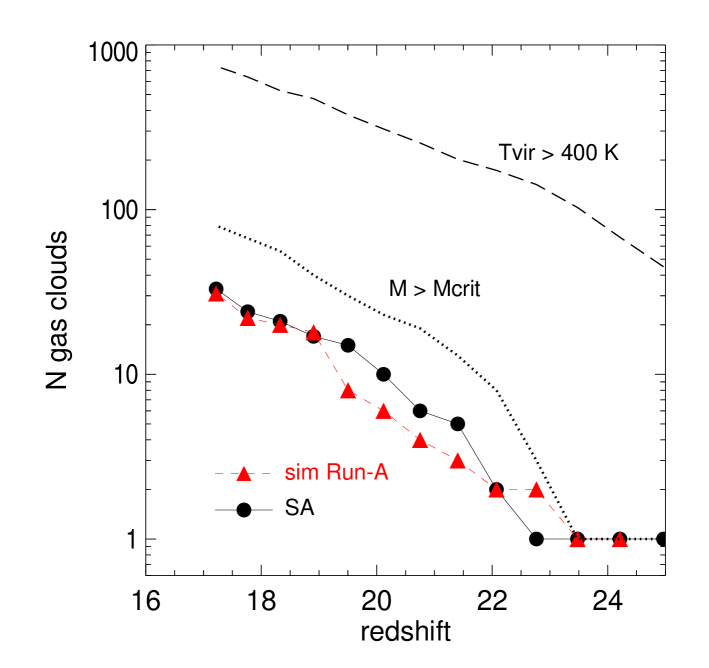
Figure 14.— The number of star-forming gas clouds. The dashed line with triangles shows the number of gas clouds found in our SPH simulation Run A. The solid line with filled circles shows the number of star-forming halos computed by applying our semi-analytic model to the dark matter halos in Run A. The dotted line is the number of halos with mass greater than the minimum collapse mass. It is about a few times larger than the number of gas clouds in the simulation. Also, for reference, we plot the number of halos with virial temperature greater than 400 K (long-dashed line); it predicts a larger number of gas clouds by more than an order of magnitude.

$$J_{\nu}(z)=\int_{z}^{z_{\rm max}}dz^{\prime}c\frac{dt}{dz^{\prime}}j_{\nu^{\prime}}(z^{\prime}),$$ (18)

where the maximum redshift for the $i$-th Lyman line at frequency $\nu_{i}$ is given by

$$\frac{1+z_{\rm max}}{1+z_{\rm observe}}=\frac{\nu_{i}}{\nu_{\rm observe}}.$$ (19)

The total source emissivity $j_{\nu^{\prime}}(z^{\prime})$ is computed by multiplying the emissivity per single star by the number of active stars at redshift $z^{\prime}$. We explore a specific model in which a single massive Population III star is formed in each cold dense gas cloud. We then use the Pop III SED computed by Bromm, Kudritzki & Loeb (2001), assuming that the stars are more massive than 100 $M_{\odot}$. For such massive stars, the luminosity per unit stellar mass is $L(\nu)\approx 3\times 10^{21}$ erg s^-1 Hz^-1 $M_{\odot}^{-1}$ in the Lyman-Werner band, with only a weak dependence on the stellar mass. Omukai & Palla (2003) argue that Population III stars with masses up to 600 $M_{\odot}$ could form by rapid accretion, whereas Abel et al. (2002) claim, based on their simulation, that a reasonable estimate for the maximum mass is 300 $M_{\odot}$. In view of the uncertainty in this quantity, we take the stellar mass to be a free parameter, keeping in mind that the total emissivity per unit volume scales as the stellar mass, provided that one massive star forms per gas cloud. We also assume that the mean lifetime of such massive stars is 3 million years (e.g. Schaerer 2002). Then, the total emissivity is given by

$$j(z)=j_{*}N_{*}(z)=j_{*}N_{\rm clouds}(z),$$ (20)

where $j_{*}$ is the emissivity per star and $N_{*}$ and $N_{\rm clouds}(z)$ are the number of active stars and the number of star-forming gas clouds at redshift $z$, respectively.

Our next task is to compute the number of star-forming gas clouds in the simulation box.

8.2. Gas cloud formation

Using the outputs of Run DM, we locate dark halos in the same manner as described in section 2 and construct a halo merger tree by tracing the formation history of individual halos (see Yoshida et al. 2002 for details). We then employ a simplified, yet physically motivated, prescription for the cooling of primordial gas within dark halos, which is also based on the results presented in the previous sections.

For all the halos at a particular redshift, we judge whether the gas within them can cool by determining if abundant numbers of hydrogen molecules have formed. Specifically, we adopt the following criteria for a halo to be star-forming: (1) the mean molecular hydrogen fraction is greater than the critical molecular hydrogen fraction, and (2) the recent mass growth rate of the halo is smaller than the critical mass growth rate. It might seem that an even simpler criterion $t_{\rm dyn}<t_{\rm cool}$ suffices for halos at a given mass. While such a model could work approximately if there is no evolving background radiation, we prefer following the merger history explicitly. It is important to specify when the gas in a halo cools, because the coupling of the increasing radiation flux with star formation makes the onset time of gas cooling critical. The above cooling criteria can be formulated as

$$f_{\rm H_{2}}(J,T_{\rm vir},z)>f_{\rm H_{2},crit},$$ (21)

and

$$\left|\frac{dT}{dt}\right|_{\rm dyn.\;heat}<\left|\frac{dT}{dt}\right|_{\rm H_{2}\;\;cooling},$$ (22)

where $f_{\rm H_{2}}(J,T_{\rm vir},z)$ is a function of the background radiation intensity $J$, the virial temperature $T_{\rm vir}$, and redshift $z$. We compute $f_{\rm H_{2}}(J,T_{\rm vir},z)$ using the asymptotic molecular fraction (equation [17] in Tegmark et al. [1997]) for no or negligible ($J_{21}<0.001$) background radiation, while we use the equilibrium H₂ abundance using equation (12), (14), (15) and (16) for background radiation with $J_{21}\geq 0.001$. The critical molecular fraction, $f_{\rm H_{2},crit}$, is computed for the virial temperature $T_{\rm vir}$ and the density of the gas within a halo. We approximate the instantaneous dynamical heating rate of a halo from its mass increase since the previous output time. The choice of the time interval for measuring the mass increase remains somewhat arbitrary. Obviously, it should not exceed either the characteristic gas cooling time or the dynamical time. We take a conservative value of 3 Myrs for the time interval, which satisfies these requirements for most of the halos. It should be noted that our model does not trace the accumulation of cold dense gas. Cold gas clouds can gradually grow in mass over a long time scale. However, describing the evolution requires specifying the gas density profile and local temperatures in a halo at a given time. Instead of following such a complicated procedure, our model simply specifies the time when an enough amount of cold gas ($\sim M_{\rm Jeans}$) is accumulated. We applied this model to our Run A by discarding gas particles and using only the dark matter particles with the particle mass scaled appropriately. We followed the halo formation history and applied the model to it. In Figure 8.1 we plot the computed number of star-forming halos against redshift. We compare it with the number of the gas clouds found in Run A. The good agreement is encouraging. We have also checked that not only do the total numbers of gas clouds agree, but that there is nearly a one-to-one match between the star-forming halos in our SPH simulation and those identified by our semi-analytic model. For reference, the number of halos with mass greater than $M_{\rm cr}=5\times 10^{5}h^{-1}M_{\odot}$ is also shown in Figure 8.1 (dotted line). The simple minimum-mass model over-predicts the number of star-forming clouds by up to a factor of three. It is worth mentioning that, in some previous works (e.g. Mackey et al. 2003), the critical virial temperature for primordial gas cloud formation was taken to be 400 K. In Figure 8.1 we plot the number of halos with virial temperature larger than 400 K. It predicts more than an order of magnitude larger (nearly two orders of magnitude at $z>22$) number of star-forming regions. This over-estimate of the number of star-forming regions would result in a substantial overestimate for the star-formation rate and associated supernova rate.

8.3. Pop III star formation at high redshift

We now couple the formation of the first stars to the evolution of the background FUV radiation so that we can predict the global star formation rate. Starting from the earliest output at $z=50$, we identify star-forming regions in the manner described in section 8.2, assuming initially that the background radiation intensity is zero. In Run DM the first star-forming region appears at $z=32$. We then determine the total emissivity within the simulation box and compute a frequency-dependent radiation flux at the next timestep according to equation (18). At every timestep, we average the radiation intensities over frequency in the Lyman-Werner band. Then, a constant radiation field with the average intensity is (assumed to be) applied. Namely, the mean intensity $\bar{J}(z)$ is used to compute the molecular hydrogen fraction in halos using equations (12) and (15), and then the cooling criteria described in section 8.2 are checked for all the halos. Figure 8.3 shows the evolution of the background radiation intensity $\bar{J}(z)$ and the spectrum of the processed radiation field $J_{\nu}$ in the Lyman-Werner band at $z=21$. The evolution of the radiation intensity is computed for two cases, one in the optically thin limit (filled circles) and the other with gas self-shielding (open squares), as described in section 7. The difference between the two cases becomes noticeable when the mean radiation intensity exceeds $\sim 10^{-24}$ erg s^-1 cm^-2 Hz^-1 str^-1. The dissociation time scale for radiation with intensity below this level is $t_{\rm diss}=k^{-1}_{\rm diss}>30$ Myrs, and thus its effect on gas cooling remains quite subtle even in the optically thin case. When the radiation intensity is above this level, it dissociates hydrogen molecules quickly and suppresses primordial gas cooling. It indeed acts more efficiently in the optically thin case and quenches star-formation more strongly. Suppressed star-formation makes the evolution of the background radiation slower than in the model with self-shielding, as seen in Figure 8.3. Interestingly, our model predicts that the mean background radiation intensity reaches a value

Figure 15.— Top panel: The evolution of the background radiation intensity for the two cases considered. The frequency averaged intensity in the range 11.18 - 13.6 eV is shown. Bottom panel: the spectrum at $z=21$ for the case with gas self-shielding. The optically thin case is quite similar except for the overall intensity level.

$10^{-23}$ erg s^-1 cm^-2 Hz^-1 str^-1 only at $z\sim 20$. This is because, as is clearly seen in the bottom panel of Figure 8.3, the hydrogen Lyman-series absorption causes a substantial intensity decrease in the Lyman-Werner band. Without the absorption, the mean intensity would have been more than an order of magnitude higher.

As we advance to lower redshifts using our model, some halos grow to have virial temperatures exceeding $T_{\rm crit.atomic}$ (see Figure 7.3). In principle, the gas should then cool via atomic hydrogen transitions even if hydrogen molecules are completely photo-dissociated. It is conceivable that a large halo will be formed through successive mergers in which molecular hydrogen cooling has never become efficient (Hutchings et al. 2001). However, we find that all the massive halos ($>M_{\rm crit.atomic}$) have a progenitor in which a star has already formed. Our model

Figure 16.— The comoving star formation rate density. Model M100 (filled circles) and model M600 (open squares).

assumes that star formation takes place only once in a halo and in its descendants during the redshift range we consider. This crudely mimics the strong radiative feedback effect due to photo-dissociation and photo-heating (Omukai & Nishi 1999; Shapiro et al. 1997) in the vicinity of the first stars. Since the physical time between $z=35$ and $=20$ is about 100 million years, the strong radiative feedback likely suppresses subsequent star formation over a significant fraction of this period (Yoshida, Abel & Hernquist 2003), unless additional processes such as metal dispersal by supernovae are invoked.

Finally, we use the number of stars formed to measure the conventional comoving star formation rate (SFR) density, $M_{\odot}$yr^-1Mpc^-3. Figure 8.3 shows our model prediction for the comoving Pop III star formation rate. We compare two cases by setting the mass of a Pop III star to be either $M_{*}=100M_{\odot}$ (filled circles, model M100) or $M_{*}=600M_{\odot}$ (open squares, model M600). We take a value of $600M_{\odot}$ for the maximum Pop III star mass from Omukai & Palla (2003). For both cases we included gas self-shielding in the model. (Thus model M100 in Figure 8.3 is the result from the same model as in Figure 8.3.) The star-formation rate density gradually increases from $z=30$ and reaches a value $\sim 10^{-3}M_{\odot}$yr^-1Mpc^-3 at $z=20$. Note that in Figure 8.3 the predicted SFR can be approximately scaled by the assumed stellar mass $M_{*}$ because of the straightforward unit conversion we used. In model M600, the star-formation rate is then about 6 times larger than in model M100. The coupling of star-formation to the evolution of the background radiation causes each to be regulated by the other (Wyse & Abel 2003). As more stars form, the radiation intensity rises, which suppresses primordial gas cooling and hence the global star-formation rate. Then, the evolution of the radiation field slows, maintaining the star formation rate at a moderate level. The flattening in the SFR for model M600 at $z<24$ is due to this regulation. It is more prominent in model M600 than in model M100 because the total emissivity per unit volume is larger in model M600.

Figure 17.— The number of halos with mass greater than $5\times 10^{5}h^{-1}M_{\odot}$ per cubic mega-parsec (comoving) volume.

We note that a characteristic feature of the Population III star-formation calculated by Mackey et al. (2003) is not seen in our result. Their model assumes a sudden quenching of star-formation, which produces a prominent “cliff” in their Figure 3. The actual regulation of the star-formation due to Lyman-Werner radiation occurs in a more complex way as we have just described, and thus the suppression of the Pop III star-formation is seen as a flattening of the star-formation rate.

Intriguingly, the predicted SFR appears quite similar to the result of the highest resolution simulation for PopIII stars by Ricotti et al. (2002a), even though their simulations and model assumptions differ from ours. Ricotti et al. (2002b) presented extensive tests using a series of simulations and examined the effect of various parameters on the global star formation rate. They showed that an important parameter which influences the SFR at $z>20$ is, indeed, the size of the simulation volume. Therefore, it is worth asking whether the finite box size of our simulation affects the overall results. While the mass resolution of Run DM is enough for our purposes (see the discussion at the beginning of this section), it is not clear if the simulated volume (a cube of 1600$h^{-1}$ kpc on a side) contains a fair sample of star-forming regions. We address this issue using the Press-Schechter halo mass function. We have verified that the mass function of the dark matter halos is reasonably well-fitted by the Press-Schechter mass function in a mass range between $10^{5}<M<10^{7}h^{-1}M_{\odot}$, and in a redshift range $20<z<30$, in agreement with Jang-Condell & Hernquist (2001) at slightly lower redshifts.

Since our analytical model relies on a one-star-per-halo assumption, we use the total number of halos with mass greater than $M_{\rm crit}=5\times 10^{5}h^{-1}M_{\odot}$ to test whether the abundance of large halos is consistent with the Press-Schechter prediction. Figure 8.3 shows the comoving number density of halos with mass greater than $M_{\rm crit}$ computed from the Press-Schechter mass function, in comparison with that found in Run DM. They agree reasonably well and the incomplete sampling of the halo mass function due to the finite box size is appreciable only at $z>30$. Figure 18.— The cosmic star formation history. We plot the star-formation rate density computed by our full semi-analytic model for $M_{*}$ = 100 $M_{\odot}$ (open circles) and for $M_{*}$ = 600 $M_{\odot}$ (open squares). The solid and dot-dashed lines are our simple functional fit (equation (23)) for the two cases. The analytic model prediction of the SFR by Hernquist & Springel (2003, their equation (2)) for the same $\Lambda$CDM cosmology is shown by the thick dashed line.
Note also that the small discrepancy remaining at lower redshifts ($20<z<30$) may be partly due to inaccuracies in the analytic mass function itself. Simulating a larger volume could make the discrepancy smaller at $z>30$, but it would not significantly alter our results because the star formation rate is not dominated by rare massive halos in our model. Therefore, we conclude that the level of agreement shown in Figure 8.3 over the relevant redshift range is satisfactory.

8.4. The cosmic star formation history

Springel & Hernquist (2003a) and Hernquist & Springel (2003) recently studied the star-formation history of a $\Lambda$CDM universe using a set of numerical simulations and an analytic model. They found that the evolution of the star-formation rate can be well described by a simple functional form. Their simulations include only the “normal-mode” of star-formation in larger mass systems, where gas cooling occurs via atomic hydrogen and helium transitions, and the regulation of star-formation is governed by supernovae rather than radiation (see Springel & Hernquist 2003b). Despite these differences, it is interesting to see how the two modes of star-formation compare at high redshift. In Figure 8.3, we compare the star-formation at very high redshifts ($20<z<30$) computed from our model and that of Hernquist & Springel (2003) for $z<20$. We show the SFR for two cases with $M_{*}=100M_{\odot}$ (open circles) and $600M_{\odot}$ (open squares). We also provide a simple functional fit in a similar spirit to Springel & Hernquist (2003a),

$$\rho_{*}(z)=\frac{1.4\times 10^{-5}M_{*}}{1+(z-17)^{0.2}\exp(0.1(z-17)^{1.5})},$$ (23)

in units of $M_{\odot}{\rm yr}^{-1}{\rm Mpc}^{-3}$. The solid line in Figure 8.3 shows equation (23) for $M_{*}=600M_{\odot}$ and the dot-dashed line is for $M_{*}=100M_{\odot}$. This simple fit describes the results of our full semi-analytic model reasonably well, as clearly seen in Figure 8.3. The SFR of Hernquist & Springel (2003) begins just at $10^{-3}M_{\odot}{\rm yr}^{-1}{\rm Mpc}^{{}_{3}}$, where our model prediction for the PopIII star formation rate ends. The overall shapes of the SFR of the two modes appear remarkably similar, although this may be just a coincidence since the physical mechanisms governing star formation and its regulation are very different in these two regimes. We also note that feedback from the first stars formed at $z\sim 20$ could affect small (proto-)galaxy formation at $10<z<20$ by photo-heating, in the same way as we argued in section 8.3. Therefore it remains unclear how the transition from Pop III to “ordinary” star-formation takes place. This issue clearly merits further study.

9. Discussions

We have carried out cosmological simulations of primordial gas cloud formation and determined the basic properties of the first baryonic objects for the standard $\Lambda$CDM cosmology. The minimum collapse mass scale is set by the fraction of molecular hydrogen produced in the primordial gas in dark matter halos, which is primarily determined by the virial temperature of the system. Our simulations reveal that the merging process of dark halos disturbs the formation and evolution of primordial gas clouds, and we detailed how such dynamical processes delay the cooling and collapse of the gas.

We have also examined the impact of far ultra-violet radiation in the Lyman-Werner bands on the formation of primordial gas clouds. We have followed the cooling and condensation of the gas within the most massive halos in one of our simulations (Run C1) for a few cases with a constant intensity radiation in the optically thin limit. Due to photo-dissociation of molecular hydrogen, gas cooling is suppressed for radiation with intensity $J_{\rm 21}>0.01$. We showed that the evolution of the gas cloud is qualitatively well-understood using a spherical collapse model. We then implemented a technique to compute molecular hydrogen column densities in and around virialized regions in the simulations and computed the gas self-shielding factor in its maximum limit. We found that, with the help of self-shielding, primordial gas in large halos cools efficiently even when irradiated by FUV radiation with intensity $J_{\rm 21}=0.01$. The overall effect of the external FUV radiation is to raise the minimum halo mass scale for efficient gas cooling. We quantified this effect using a large volume simulation (Run A) and found that, in the optically thin limit, the influence of FUV radiation can be formulated using an equilibrium H₂ abundance. Furthermore, we found that gas self-shielding can also be described by defining an effective shielding factor in a simple manner. While our experiments in the two extreme cases, the optically thin limit and with maximal gas self-shielding, should bracket the true effect of gas self-shielding, a more detailed study is needed to obtain an accurate estimate of this process. A promising approach may be to discard high velocity gas elements in computing molecular hydrogen column densities (Simon Glover, private communication).

Ideally, one would like to perform $N$-body hydrodynamic simulations with gas chemistry and radiation using a large number of particles to study the coupling of star formation to the evolution of the radiation field. Unfortunately, to simulate a volume equivalent to our dark matter simulation Run DM with the same resolution as our Run A, would require at least $2\times 768^{3}$ particles. As an alternative, we developed a semi-analytic model for primordial gas cooling and gas cloud formation. By comparing our model predictions with the results of SPH simulations, we found that the model reproduces the number of primordial gas clouds in the simulated volume very well. We then successfully applied it to outputs of a large $N$-body simulation. Assuming a simple star formation-law, we have computed the star formation rate and the evolution of the background radiation at high redshift ($20<z<35$). We believe that our model can be used to reliably estimate the rate of events associated with star formation, such as supernovae and gamma-ray bursts.

While our simulations include the physics needed to study basic properties of the first star-forming clouds, there are still a few additional mechanisms that could be important. An interesting possibility proposed by Haiman et al. (2000) and Oh (2001) is that an early X-ray background could increase the number of free electrons in the IGM and promote the production of hydrogen molecules. Analytical estimates (Haiman et al. 2000) and numerical simulations (Machacek et al. 2003) indicate, however, that the net effect is mild and the positive feedback by an X-ray background does not entirely compensate the negative feedback effect due to photo-dissociating Lyman-Werner radiation unless unreasonably high X-ray intensities are assumed. It thus appears that our model prediction for the star-formation rate should be robust, even without additional contributions from X-ray sources. It is probably more important to include direct radiative transfer effects from the first stars. In the present model, we only crudely included the overall effect by quenching further star formation locally after the first star is formed. In our simulations we find that many gas clouds are located close to one another, with physical separations smaller than 10 kpc. These star forming clouds at high redshifts are, as we have shown, embedded in dark halos that are strongly clustered (see Figure 2). A single massive population III star can ionize a large volume of the surrounding IGM and thus can have considerable impact on the formation of the nearby gas clouds and stars. In a forthcoming paper we will study direct radiative transfer effects using ray-tracing simulations.

APPENDIX : Time Stepping in SPH with Non-equilibrium Chemistry

We describe the time step criterion that incorporates the non-equilibrium nature of the physics in our simulations. The code GADGET employs an individual time step scheme and the usual time step criterion for the $i$-th gas particle is given by the Courant condition

$$\Delta t_{i}=\frac{\alpha_{\rm cour}h_{i}}{h_{i}|(\nabla\cdot{\bf v})_{i}|+\max(c_{i},|{\bf v}_{i}|)(1+0.6\alpha_{\rm visc})},$$ (24)

where $h_{i},c_{i},{\bf v}_{i}$ have their usual meanings (see Springel et al. 2001), $\alpha_{\rm visc}$ regulates the strength of the artificial viscosity, and $\alpha_{\rm cour}$ is the Courant factor. For each gas particle, we supplement this criterion with two additional constraints so that the time step does not exceed the gas cooling time and the characteristic chemical reaction time. We monitor the cooling time

$$\Delta t_{\rm cool}=e_{\rm tol}\frac{\;T\;}{\;\dot{T}\;}$$ (25)

and use the rate of change of the electron number density to judge the characteristic chemical reaction time

$$\Delta t_{\rm chem}=e_{\rm tol}\frac{\;n_{\rm elec}\;}{\;\dot{n}_{\rm elec}\;}.$$ (26)

We set the tolerance parameter $e_{\rm tol}=0.1$ throughout the simulations.

References

- (1) Abel, T., Anninos, P., Norman, M. L., & Zhang, Y. 1997, New Astronomy, 2, 181
- (2) Abel, T., Anninos, P., Norman, M. L., & Zhang, Y. 1998, ApJ, 2, 181
- (3) Abel, T., Bryan, G. L., & Norman, M. L. 2002, Science, 295, 93
- (4) Barkana, R. & Loeb, A. 2000, ApJ, 539, 20
- (5) Barkana, R. & Loeb, A. 2001, Physics Report
- (6) Bromm, V., Coppi, P. S., & Larson, R. B. 2002, ApJ, 564, 23
- (7) Bromm, V., Kudritzki, R. P., & Loeb, A. 2001, ApJ
- (8) Bullock, J. S., Dekel, A., Kollat, T. S., Kravtsov, A. V., Klypin, A. A., Porciani, C, & Primack, J. R. 2001, ApJ, 555, 240
- (9) Cen, R. 2003, ApJ, in press
- (10) Couchman, H. M. P. & Rees, M. J. 1986, MNRAS, 221, 53
- (11) Ciardi, B., Ferrara, A., Governato, F. & Jenkins, A., 2000, MNRAS, 314, 611
- (12) Christlieb, N., Bessel, M. S., Beers, T. C., Gustafsson, B., Korn, A., Barklem, P. S., Karlsson, T., Mizuno-Wiedner, M., & Rossi, S. 2002, Nature, 419, 904
- (13) Dekel, A & Rees, M. J. 1987, Nature, 326, 455
- (14) Drain, B. T. & Bertoldi, F. 1996, ApJ, 468, 269
- (15) Fan, X., et al. 2000, AJ, 120, 1167
- (16) Fukugita, M. & Kawasaki, M. 1991, MNRAS, 269, 563
- (17) Fuller, T. M. & Couchman, H. M. P. 2000, ApJ, 544, 6
- (18) Galli, D. & Palla, F. 1998, A&A, 335, 403
- (19) Glover, S. C. O. & Brand, P. W. J. L., 2001, MNRAS, 321, 385
- (20) Gnedin, N. 2000, ApJ, 535, 530
- (21) Gnedin, N. & Ostriker, J. P. 1997, ApJ, 486, 581
- (22) Haiman, Z., Rees, M. J., & Loeb, A. 1996, ApJ, 467, 522
- (23) Haiman, Z., Rees, M. J., & Loeb, A. 1997, ApJ, 476, 458
- (24) Haiman, Z., Abel, T., & Rees, M. J. 2000, ApJ, 534, 11
- (25) Hernquist, L. & Springel, V. 2003, MNRAS, submitted (astro-ph/0209183)
- (26) Hutchings, R. M., Santoro, F., Thomas, P. A. & Couchman, H. M. P. 2002, MNRAS, 330, 927
- (27) Jang-Condell, H., & Hernquist, L. 2001, ApJ, 548, 68
- (28) Jenkins, A., Frenk, C. S., White, S. D. M., Colberg, J. M., Cole, S., Evrard, A. E., Couchman, H. M. P., Yoshida, N., 2001, MNRAS, 321, 372
- (29) Kashlinsky, A. & Rees, M. J. 1983, MNRAS, 205, 955
- (30) Kauffmann, G., Colberg, J. M., Diaferio, A. & White, S. D. M., 1999, MNRAS, 303, 188
- (31) Kitayama, T., Susa, H., Umemura, M. & Ikeuchi, S. 2001, MNRAS, 326, 1353
- (32) Loeb, A. & Barkana, R. 2001, ARA&A, 39, 19
- (33) Machacek, M. E., Bryan, G. L., & Abel, T. 2001, ApJ, 548, 509
- (34) Machacek, M. E., Bryan, G. L., & Abel, T. 2003, MNRAS, 338, 273
- (35) Mackey, J., Bromm, V., & Hernquist, L. 2003, ApJ, 586, 1
- (36) Matsuda, T, Sato, H & Takeda, H. 1969, Prog. Theor. Phys., 41, 840
- (37) Oh, S. P. 2001, ApJ, 569, 558
- (38) Omukai, K. & Nishi, R. 1998, ApJ, 508, 141
- (39) Omukai, K. & Nishi, R. 1999, ApJ, 518, 64
- (40) Omukai, K. 2001, ApJ, 546, 635
- (41) Omukai, K. & Palla, F. 2003, submitted to ApJ
- (42) Ricotti, M., Gnedin, N. Y., & Shull, J. M. 2001, ApJ, 560, 580
- (43) Ricotti, M., Gnedin, N. Y., & Shull, J. M. 2002a, ApJ, 575, 33
- (44) Ricotti, M., Gnedin, N. Y., & Shull, J. M. 2002b, ApJ, 575, 49
- (45) Santos, M. R., Bromm, V. & Kamionkowski, M. 2002, MNRAS, 336, 1082
- (46) Schaerer, D. 2002, A&A, 382, 28
- (47) Seager, S., Sasselov, D. D. & Scott, D. 2000, ApJ, 128, 407
- (48) Shapiro, P. R., Raga, A. C. & Mellema, G. 1997, in Proceedings of the 13th IAP Astrophysics Colloquium, eds. P. Petitjean and S. Charlot
- (49) Sokasian, A., Hernquist, L., Abel, T. & Springel, V. 2003, astro-ph/0303098
- (50) Springel, V., Yoshida, N. & White, S. D. M. 2001, New Astronomy, 6, 79
- (51) Springel, V. & Hernquist, L. 2002, MNRAS, 333, 649
- (52) Springel, V. & Hernquist, L. 2003a, MNRAS, 339, 312
- (53) Springel, V. & Hernquist, L. 2003b, MNRAS, 333, 289
- (54) Sugiyama, N. 1995, ApJ, 100, 281
- (55) Tegmark, M., Silk, J., Rees, M., Blanchard, A., Abel, T., & Palla, F. 1997, ApJ, 474, 1
- (56) van den Bosch, F., Abel, T., Croft, R., White, S. D. M, & Hernquist, L. 2002, ApJ, 576, 21
- (57) Venkatesan, A., Tumlinson, J. & Shull, J. M. 2003, ApJ, in press
- (58) Vitvitska, M., Klypin, A. A., Kravtsov, A. V., Wechsler, R. H., Primack, J. R. & Bullock, J. S., 2002, ApJ, 581, 799
- (59) White, S. D. M. & Rees, M. J. 1978, MNRAS, 183, 341
- (60) White, S. D. M. & Springel, V. 1999, in First Stars, Proc. of the MPA/ESO workshop, eds. Weiss, A., Abel, T. & Hill, V.
- (61) Wyithe, J. S. & Loeb, A. 2003a, ApJ, in press
- (62) Wyithe, J. S. & Loeb, A. 2003b, ApJL submitted (astro-ph/0302297)
- (63) Wyse, J. & Abel, T. 2003, to appear in Proceeding of the 13th October Conference
- (64) Yoshida, N., Abel, T. & Hernquist, L. 2003, in preparation
- (65) Yoshida, N., Stoehr, F., Springel, V. & White, S. D. M. 2002, MNRAS, 335, 762
- (66) Yoshida, N. & Sugiyama, N. 2003, submitted to MNRAS